the Creative Commons Attribution 4.0 License.
the Creative Commons Attribution 4.0 License.
 | 27 Jul 2018
Development and assessment of uni- and multivariable flood loss models for Emilia-Romagna (Italy)
Francesca Carisi
Kai Schröter
Alessio Domeneghetti
Heidi Kreibich
Attilio Castellarin
Flood loss models are one important source of uncertainty in flood risk assessments. Many countries experience sparseness or absence of comprehensive high-quality flood loss data, which is often rooted in a lack of protocols and reference procedures for compiling loss datasets after flood events. Such data are an important reference for developing and validating flood loss models. We consider the Secchia River flood event of January 2014, when a sudden levee breach caused the inundation of nearly 52 km2 in northern Italy. After this event local authorities collected a comprehensive flood loss dataset of affected private households including building footprints and structures and damages to buildings and contents. The dataset was enriched with further information compiled by us, including economic building values, maximum water depths, velocities and flood durations for each building. By analyzing this dataset we tackle the problem of flood damage estimation in Emilia-Romagna (Italy) by identifying empirical uni- and multivariable loss models for residential buildings and contents. The accuracy of the proposed models is compared with that of several flood damage models reported in the literature, providing additional insights into the transferability of the models among different contexts. Our results show that (1) even simple univariable damage models based on local data are significantly more accurate than literature models derived for different contexts; (2) multivariable models that consider several explanatory variables outperform univariable models, which use only water depth. However, multivariable models can only be effectively developed and applied if sufficient and detailed information is available.


According to analyses of the Centre for Research on the Epidemiology of Disasters (CRED), hydrological disasters (i.e., natural disasters caused by river and coastal floods, flash floods, rainstorms) are the most frequently recorded natural calamities occurring worldwide in the last 2 decades (see, e.g., Guha-Sapir and CRED, 2015). Also, the number of disasters caused by hydrological events in 2016 exceeded by far that of any other type of natural hazards (Guha-Sapir and CRED, 2016).
Flooding was the third major cause of economic loss worldwide among all natural disasters between 2006 and 2015 (the firsts were earthquakes and storms), resulting in total damages larger then USD 300 billion. In Europe, the proportion of flood impacts was even larger during the same decade, with inundations ranked first in terms of total damage (i.e., USD ∼51 billion; CRED). The CRED findings about the increasing amount of economic loss starting from the second half of 20th century agree with the analyses carried out by the Intergovernmental Panel on Climate Change (IPCC), which highlighted that flood damages in the past 10 years were 10 times higher than in the period 1960–1970 (IPCC, 2001, 2014).
Future scenarios provided by IPCC (2014) and Jongman et al. (2012) suggest that extreme flood events at a global scale are expected to increase in terms of frequency and magnitude. Barredo (2009) drew a hypothetical scenario without any change in the meteorological forcing and found that loss would increase anyway in the future due to exposure and socioeconomic changes (e.g., higher demographic pressure, improved per capita wealth and living standards).
The implementation of the European Union Floods Directive (2007/60/EC) led flood risk assessment and management to gain even greater interest (de Moel et al., 2015; Dottori et al., 2016b, and references therein), forcing member states and authorities to dedicate additional resources and efforts to the assessment, mitigation and management of flood risk in the broader contexts of possible climate change, population growth and economic changes (Meyer et al., 2013; Merz et al., 2010, 2014). However, despite these efforts, there are still several open problems and limits that need to be discussed and addressed in order to better assess flood risk and its evolution in time and space.
Among the three components that define flood risk (hazard, exposure and susceptibility), this paper focuses in particular on the last two, namely the qualification and quantification of the exposed elements and the attribution of a loss value to them, as a function of one or more flood intensity parameters and resistance characteristics (damage models). The scientific literature of the last decade shows a large number of innovative damage models that are capable of estimating flood loss starting from one or more predictive variables. Nevertheless, several authors indicate that damage models still provide an important source of uncertainty in flood damage estimates, leading to uncertainties which are comparable to or larger than those associated with any other component (Jongman et al., 2012; de Moel et al., 2012, 2014; Gerl et al., 2016; Merz et al., 2004, 2007; Apel et al., 2009).
One important source of uncertainty is the simplified representation of complex damaging processes in terms of a stage-damage function (Jongman et al., 2012). Since White (1945) linked the water level to relative (i.e., the loss ratio) or monetary damages, most of the models used today stick to this concept, using only water depth to estimate relative loss (see, e.g., Penning-Rowsell et al., 2005; Smith, 1994; Apel et al., 2009; Kreibich et al., 2009; Merz et al., 2013). Other important influencing factors, such as flood duration and flow velocity, are often not considered (de Moel and Aerts, 2011; Merz et al., 2013). Recently, some authors (see Merz et al., 2013; Chinh et al., 2016; Hasanzadeh Nafari et al., 2016, 2017; Kreibich et al., 2017; Spekkers et al., 2014) developed multiparameter damage models including more than one predictive variable, chosen among other hydraulic parameters (e.g., streamflow velocity, duration of the inundation), resistance performance, precautionary measures, and people's awareness of and experience with floods (Meyer et al., 2013). These models were shown to outperform univariable loss models, under the condition that sufficiently large and detailed damage datasets are provided (Merz et al., 2013; Schröter et al., 2016). Bubeck and Kreibich (2011), Cammerer et al. (2013), Messner et al. (2007), and Meyer et al. (2013), among others, indicate the need for a better understanding of the damage processes as a means to further improve multivariable models.
A further aspect that contributes to the overall uncertainty in flood risk assessment and modeling is the lack of sufficient, comparable and reliable high-quality flood loss data (Meyer et al., 2013; Molinari et al., 2014a; Amadio et al., 2016; Scorzini and Frank, 2015; Green et al., 2011). In the absence of empirical damage data, loss models are either selected from the literature or subjectively and schematically derived by experts using a synthetic approach (see, e.g., Penning-Rowsell et al., 2005; Merz et al., 2004, 2013; Thieken et al., 2008; Kreibich et al., 2010; Dottori et al., 2016a). In fact, data collected in the events' aftermath are crucial to construct new models and validate existing ones (Meyer et al., 2013; Cammerer et al., 2013; Ballio et al., 2015), to adjust them for peculiar conditions of the study area, to improve the consistency of the models themselves (Amadio et al., 2016; Büchele et al., 2006; Gerl et al., 2016) and to provide information about their transferability in different analyses and contexts (Molinari et al., 2014a; Cammerer et al., 2013; Green et al., 2011). Many damage models developed up to now are in fact internationally accepted as standard methodologies for estimating flood damages (Merz et al., 2007, 2010; Smith, 1994), without being either tested or calibrated for the specific study area (Amadio et al., 2016). Indeed, using damage models for geographical areas, socioeconomic conditions and flood events that differ from those for which the models themselves have been originally derived leads to the incorporation of large errors into the assessment of flood risk (Merz et al., 2004; Schröter et al., 2016; Merz et al., 2010). According to Gerl et al. (2016), validation analyses were performed only for about 45 % of literature models included in their review by means of comparisons with observed data, while for the remaining models either the evaluation status is unknown or the validation process is not explicitly described.
Concerning Italy, the scientific literature reports, on the one hand, several examples in which models developed elsewhere are applied without calibration or validation (see, e.g., Amadio et al., 2016), and on the other hand it clearly states the limited exportability of empirical damage models (see, e.g., Molinari et al., 2014b, on the transferability of the model developed on the basis of specific flood event data by Luino et al., 2006 and Freni et al., 2010). Molinari et al. (2012) associate the generalized poor performance of loss models with a variety of reasons, among which two are worth recalling. First, the Italian peninsula is characterized by an extreme variability in geographical and geomorphological contexts as well as in urban textures and building typologies. Second, Italian flood loss datasets are generally of low quality and very often characteristic of small areas, if compared to other European case studies (see Molinari et al., 2012).
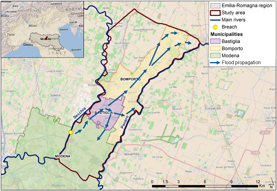
Figure 1Study area, Secchia and Panaro rivers, location of the breach (yellow dot), municipalities of interest (i.e., Bastiglia, Bomporto and Modena) and a schematic of the inundation dynamics.
The analysis described herein assesses the performance of uni- and multivariate empirical models developed on the basis of a recently compiled Italian dataset. Our study highlights the problem of lacking consistent data and the consequent difficulty in the development of robust and reliable damage models for estimating flood loss to buildings and contents in local applications. Furthermore, our study contributes to the understanding of potential and limitations of flood damage modeling in northern Italy, aiming at investigating the open problem of transferability of empirical damage models to different areas and socioeconomic contexts.
We consider one of the most comprehensive Italian flood damage datasets, which consists of 1330 post-event data on flooded private properties in the province of Modena (northern Italy), collected in the aftermath of the Secchia River inundation (January 2014). The database contains information about the affected properties, such as their location and structural characteristics and the amount of loss suffered, concerning both structural and nonstructural parts and installations (termed “buildings” from here on) and furniture and household appliances (“contents”) of each building (see Sect. 3.1 and 3.2). The raw data collected by local authorities have been homogenized, geocoded and integrated with other useful information including the outcomes of a detailed hydrodynamic numerical simulation of the inundation event (see Sect. 3.3).
Our study is structured into three main components.
-
First, concerning direct tangible economic damages to buildings, we use the above dataset to derive uni- and multivariable damage models for the study area and compare the accuracy in estimating damages with a selection of established literature models.
-
Second, we calibrate empirical uni- and multivariable models to subsections of the study area and validate them using the data observed in different subsections (split-sample validation).
-
Third, we investigate the relationship between damages to buildings and damages to contents, also developing an empirical damage model for the latter.
Our study focuses on a real inundation event that occurred in Italy in 2014 and was caused by a breach in the right embankment of the Secchia River during an intense, yet not extreme, flood event. The collapse of the right levee occurred on 19 January near the town of San Matteo, in the northern part of the Modena municipality (see yellow dot in Fig. 1) and caused the inundation of the neighboring municipalities of Bastiglia, Bomporto and Modena (violet, orange and green polygons in Fig. 1, respectively) in less than 30 h. The overflowing volume was estimated at between 36.3×10⁶ and 38.7×10⁶ m3, flooding an area of about 52 km2 (see, e.g., Orlandini et al., 2015). Towns and the surrounding countryside remained flooded for more than 48 h, until a water volume in excess of 20×106 m3 was finally pumped out of the inundated area. According to Orlandini et al. (2015), the total estimated flood loss was about EUR 500 million (about EUR 16 million considering only residential properties).
The study area includes the municipalities of Bomporto and Bastiglia and the northern part of the municipality of Modena. It is located on the Secchia downriver on the right side and it extends for approximately 112 km2. The area is mainly flat and the main relieves consist of roads or railway embankments and minor river levees. The aspect of the area is oriented in a northeastern direction, along which ground elevations decrease from ca. 30 m a.s.l. in the southwestern territories to ca. 18 m a.s.l. about 20 km northeastwards.
The delineation of the study area relies on different topographic boundaries. The western boundary in Fig. 1 is the right levee of the Secchia River, while the eastern boundary consists of the left levee of the Panaro River, which also flows towards the northeast, almost parallel to the Secchia River. Roads, embankments and drainage channels which form the southern and northern boundaries are an important control for flooding dynamics (Carisi et al., 2017) and, in the northern part, they prevented urban areas from being flooded.
The breach was first detected at 06:30 LT. Most likely it was triggered either by direct river inflow into the riverside entrance of an animal burrow system or by the collapse of an existing animal burrow, which was separated by a 1 m earthen wall from the levee riverside and saturated during the flood event (Orlandini et al., 2015). A trapezoidal part of the embankment, with a base width of about 10 m, was removed and the embankment's top elevation became immediately 1 m lower than the river water surface. The breach reached a maximum bottom width of about 80 m and the embankment's top elevation became equal to the ground level within 9 h (15:00 LT of 19 January 2014). Given the advanced state of the development of the breach when it was first discovered, no repair of the breached levee was even attempted as an immediate measure.
Thanks to several eyewitness accounts, video footage and studies conducted by an ad hoc scientific committee (D'Alpaos et al., 2014; DICAM-PCREM, 2015), it was possible to identify the flood event propagation dynamics, shown by the blue arrows in Fig. 1. These data were used, together with local accounts, pictures and videos of the flooded municipalities, to reconstruct the event by means of a fully 2-D hydrodynamic model (see Sect. 3.3).
In the immediate post-event period, for the purpose of compensation, authorities of the Emilia-Romagna region, Modena Province and affected municipalities started a data collection campaign to obtain as much information as possible on the damages caused by the flood event. According to regional decree no. 8 of 24 January 2014, the aim of the survey was to quantify the financial needs for the restoration of damaged public buildings, infrastructure network, hydraulic and hydrogeological works, and private properties for residential use, household contents, private registered goods and goods related to the productive sector. Accordingly, citizens and property owners were asked to fill out forms about public property damages, private properties, furniture and registered goods damages, and damages to the economic and productive activities and agriculture and agro-industrial sectors. In the present analysis, damage assessment focuses exclusively on private properties.
Table 1Number of forms filled by private owners per municipality.
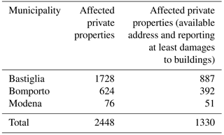
Authorities collected a total of 448 forms, divided as per the affected municipalities. In order to geocode the position of every damaged property, the complete database was filtered, considering only records for which the complete address was provided. The database regards private properties affected by different kinds of potential damages: damages to buildings (structural and nonstructural parts and installations), content damages (furniture and household appliances), and structural damages to common parts and registered goods damages (cars, motorcycles, etc.). Our analyses focus only on properties affected at least by damages to buildings. The total number of considered forms is therefore 1330 (see Table 1, second column).
The 1330 records were geocoded in a GIS environment, using the Google Maps base map, this being one of the most complete freely available maps for the study area; geocoding was followed by a careful manual control activity using publicly available internet pictures, Google Street View and Google Earth. This step enabled the correction of several wrong or inaccurate geocodings, mainly in the rural areas, where distances between street numbers are higher.
Table 2Refundable assets in accordance with ordinance no. 2 of 5 June 2014 and law no. 93 of 26 June 2014.
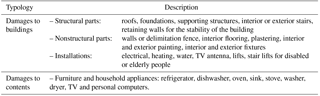
Table 3Considered variables and their sources and ranges, for building and content damage analysis.
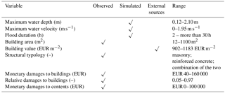
The refund requests by citizens, collected from municipal authorities, were divided into different asset typologies: building damages, content damages, and structural damages to common parts and registered goods. We neglected structural loss to common parts and registered goods in our analyses because of the limited number of data collected on these categories. Table 2 shows in detail the different assets which could be refunded for building and content damages. Table 3 summarizes all data collected and used in our study for each damaged property, providing information about the original sources and grouping the data into three different categories: observed (i.e., declared by owners in the official forms), simulated by the hydrodynamic model and retrieved from an external source. The rightmost column of the same table reports the ranges of these variables within the study area. The following subsections detail the information collected and summarized in Table 3.
3.1 Damages to buildings
As mentioned before, all 1330 considered records report at least damages to buildings (structural and nonstructural parts and installations). Authorities defined the final compensation granted to owners in accordance to ordinance no. 2 of 5 June 2014 and law no. 93 of 26 June 2014, which specifies refund criteria. For instance, considering the total amount of money that authorities had available for the restoration of all kinds of properties, the maximum coverage for each property was set to EUR 85 000 for damages to buildings and EUR 15 000 for damages to contents, setting a fixed amount of money for each room. In addition, owners declarations about the amount of the restoration work of the damaged parts, if higher than EUR 15 000, were verified by authorities by means of expert technical reports. These controls probably reduced the amount of damage claimed by owners, who commonly tend to overestimate their loss and have less competency for estimating damages than professionals have.
Nevertheless, the limited availability of money and the need for a homogeneous criterion for all the affected properties led in many cases to a much higher reduction of the amount of damage refundable to the owners. In fact, refundable assets are only a cut percentage of assets that can be found in a property and, in addition, experienced damages could be higher than the maximum coverage established by authorities. The difference between overall monetary refunded and claimed damages to buildings is equal to about EUR 1.7 million (EUR 15.2 million of declared loss vs. EUR 13.5 million of refunded loss). Given this significant difference, in order to preserve the representativeness and consistency in loss data, we chose to consider observed damages in our study as claimed by citizens in the forms they filled (estimation of the financial need for restoration, without knowing the refund criteria). We are aware that this choice can introduce overestimation of the damages (particularly considering damages below EUR 15 000) for the reason explained before, but we considered this possible error having less influence on loss estimation, both quantitatively and methodologically, relative to the distortions that would be systematically introduced by adopting the result of the compensation phase.
Together with the amount of money requested for compensation, we also extracted from the filled forms the available information on building footprints and structural typology (masonry, reinforced concrete, etc.) because of their potential impact on the damage process and therefore on damage modeling (see also previous studies, e.g., Merz et al., 2013).
In order to evaluate loss in relative terms (as the percentage of suffered damage relative to the total value of the building), we retrieved the economic value of each property from the Italian Revenue Agency reports (Agenzia delle Entrate, AE, 2018). Every 6 months the AE issues the open-market values (EUR m−2) for different assets (e.g., civil houses, offices, stores) in each Italian administrative district (spatial scale of municipality), taking into account different classes of residential and industrial buildings and the overall economic well-being of the region. These values are different for each homogeneous geographical area (OMI zone) and set a minimum and a maximum market value per unit area. Focusing on residential buildings, and in particular on their structural part without including the cost of the land, we defined the buildings' economic value (EUR m−2) as the average of the values provided for each building in the same OMI zone. Only the first floor of each building was considered since the maximum water depth is always lower than or equal to 2.1 m (see Table 3). It is important to notice that these economic values do not consider a possible fall in price due to catastrophic events. Also, we are aware that reconstruction costs seem to be more suitable for this kind of analyses, but they are not freely available in Italy or homogeneous at a national level, different from OMI values. Moreover, the use of these economic values at an aggregation level is still informative for future ex ante damage estimation for planning activities and it is in line with previous loss analyses at different scales (see, e.g., Arrighi et al., 2013; Domeneghetti et al., 2015).
3.2 Damages to contents
We also analyze the monetary loss to household un-registered contents (e.g., furniture and household appliances: refrigerator, dishwasher, oven, sink, stove, washer, dryer, TV and personal computers).
Focusing on these data and looking at the refunded loss, because of the stricter criteria for content damage compensation of ordinance no. 2 of 5 June 2014 and law no. 93 of 26 June 2014, the difference between the requested and refunded amount is even more evident. It is equal to about EUR 5.7 million (EUR 10.4 million of overall declared loss to contents vs. EUR 4.7 million of refunded loss) and confirms the choice to consider observed damages as claimed by owners.
Concerning this dataset, it is worth noting that we do not have any specific information for each building on the items recorded under the generic expression “contents”. Therefore, we cannot express these damages in terms of relative loss over the overall movable property value. Also, the damage models to household contents proposed by the scientific literature are fairly rare and isolated (some examples are represented by studies performed by Penning-Rowsell et al., 2010; Thieken et al., 2008). Thus, we investigate the usefulness of an indirect modeling approach, which is based on regressing loss to contents against loss to buildings (see Sect. 5.3), for this type of damage.
3.3 Hydrodynamic characterization of the inundation event
Forms collected from authorities for the purpose of compensation do not include data on hydraulic variables, such as water depth, water velocity, etc. Since these data are necessary for our analysis, the reconstruction of the flood event is performed by means of TELEMAC-2D, a fully 2-D hydrodynamic model which solves the 2-D shallow water Saint-Venant equations using the finite-element method within a computational mesh of triangular elements (see Galland et al., 1991; Hervouet and Bates, 2000, for details). This computational model complies with the validation protocol by the International Association for Hydro-Environment Engineering and Research (IAHR) and has been successfully applied to case studies around the globe (Hervouet and Bates, 2000; Brière et al., 2007).
Concerning the inundation event, the dynamics of the wetting front were strongly influenced by the presence of topographic discontinuities (e.g., road embankments, artificial as well as natural channels belonging to the minor stream network; see D'Alpaos et al., 2014). In order to correctly reproduce ground elevation and discontinuities in the model, a detailed lidar DEM with a spatial resolution of 1 m is used and an unstructured triangular finite-element mesh of the study area is generated. The mesh consists of 34 082 nodes connecting 66 596 elements with variable length side from 1 to 200 m in flatter zones, covering a total of 112 km2. This accurate mesh ensures the correct representation of all major linear discontinuities existing in the study area.
The outflowing hydrograph of the levee breach, as reconstructed by the scientific committee that studied the event (D'Alpaos et al., 2014), is used as a boundary condition, in particular as inflow to the boundary elements representing the levee breach.

Figure 2Maximum water depths simulated by the 2-D model; geolocated building damages (colors reflect municipalities).
The calibration of the 2-D model is performed by varying floodplain roughness coefficients in order to reproduce the real extent of the inundation, at different time steps, as documented by maps and aerial images made available immediately post event by competent authorities and rescuers (D'Alpaos et al., 2014), and as also confirmed by later studies (see, e.g., Vacondio et al., 2016). In particular, Manning's coefficient values were differentiated between agricultural areas and urban areas, and resulting coefficients (0.033 and 0.1 m s, respectively) are in line with values reported in the scientific literature (see, e.g., Vorogushyn, 2008; Domeneghetti et al., 2013).
After the event, local authorities collected information about water depths reached at different points of the inundated area. This information is used for the validation of the model, together with pictures, videos and reports made available on the Internet, as well as through in situ interviews. At about 50 points, uniformly distributed in the study area, simulation outcomes are compared in terms of water depth with the information available. Results show a good agreement between simulated and observed flooding dynamics, with the residuals between observed and simulated water levels always smaller than ±20 cm. In order to avoid errors due to the model uncertainty, we consider the area with simulated water depth greater than 10 cm to be “flooded” (see, e.g., Castellarin et al., 2009; Samuels, 1995).
The calibrated and validated model is then used to reconstruct the detailed spatiotemporal dynamics of the inundation event and to identify the spatial distribution of the hydraulic variables of interest. In fact, combining 2-D model outcomes and geocoded locations shown in Fig. 2, it is possible to extract maximum water depth, maximum flow velocity and duration of the inundation at each site (see Table 3). Maximum water depth and the maximum flow velocity commonly refer to different time steps of the flood event.
As already discussed in Sect. 1, damage models return the amount of loss potentially suffered by certain elements (population, buildings, economic activities, ecosystem, etc.) as a result of a specific flood event, thus providing an estimate of the objects' susceptibility. These models associate relative (or monetary) loss with different input variables. The most frequently used loss models in Europe are univariable damage models, i.e., they estimate the amount of damage as a function of a single input variable, most commonly water depth (Merz et al., 2010; Messner et al., 2007; Jongman et al., 2012), distinguishing among different building uses, types, etc. (Gerl et al., 2016). Although each model is developed with different approaches and uses different economic values for assets, the damage values can be relativized based on each different context in order to make the models comparable to each other.
This section briefly recalls well-known and largely employed literature depth–damage models (also called stage-damage models, shown in Fig. 3). Furthermore, it describes empirical depth–damage models and a multivariable loss model that we derived for the Secchia loss dataset. All uni- and multivariable models illustrated here are applied for predicting loss to buildings and household contents resulting from the January 2014 Secchia flood event.
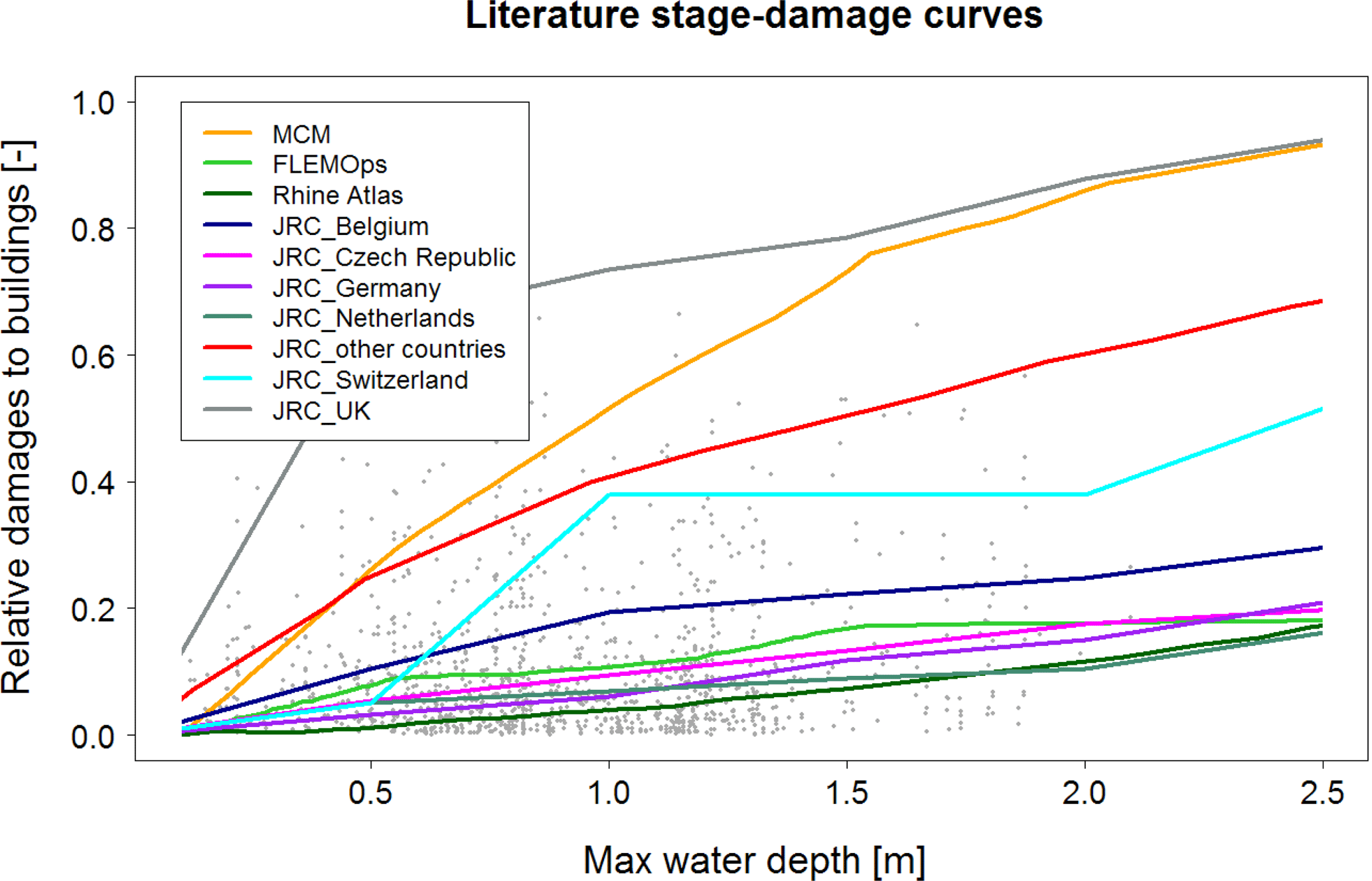
Figure 3Literature stage-damage models and observed data: grey points in the background represent the observed relative loss (buildings only); literature models are limited to the maximum water depth reconstructed for the inundation event through the 2-D hydrodynamic model (i.e., 2.5 m).
4.1 Literature damage models
4.1.1 Multi-Coloured Manual (MCM) model
The depth–damage curve implemented in the Multi-Coloured Manual (MCM; Penning-Rowsell et al., 2005) is considered to be one of the most comprehensive and detailed models for flood damage estimation in Europe and it is used as a support for water management policy and quantitative assessment of the effect of investment decisions (Penning-Rowsell et al., 2010; Jongman et al., 2012). This model estimates loss based almost exclusively on synthetic analysis and expert judgment from the insurance industry or engineers (Penning-Rowsell et al., 2005; Bubeck and Kreibich, 2011). Different from the majority of other damage models, MCM estimates building damages using a monetary depth–damage curve, i.e., it defines monetary potential loss relative to water depth, rather than providing damage ratios (Penning-Rowsell et al., 2005; Bubeck and Kreibich, 2011; Jongman et al., 2012). Similar to previous studies (see, e.g., Domeneghetti et al., 2015) and aiming at performing a fair comparison among all considered models, we make use of the relative depth–damage curve as obtained by Jongman et al. (2012), who rescaled the original MCM monetary curve by referring the total building damage (100 %) to an average pre-flood depreciated building value in 2005 pound sterlings (GBP) (see Table 2 in Jongman et al., 2012).
4.1.2 Flood Loss Estimation MOdel for the private sector (FLEMOps)
The Flood Loss Estimation MOdel for the private sector (FLEMOps) (Thieken et al., 2008) is an empirical model based on an extensive dataset from 2158 private households that were significantly affected by flood events in 2002, 2005 and 2006 in Germany. According to Thieken et al. (2008), the database used for identifying FLEMOps was compiled through computer-aided telephone interviews with a sample of people affected by these serious events. FLEMOps assesses relative flood damages to private households by referring to several factors: inundation depth, building type, building quality, water contamination and private precaution. Although the original FLEMOps was developed as a multivariable model, in this study we implemented it as a univariable one, by referring to the water depth as the only parameter available in our data collection. The curve taken into account in this study (see Fig. 3) is the one that considers a uniform distribution of building types in the study area (see Apel et al., 2009), while no information about building quality, water contamination and private precaution was available (concerning these last three factors, the first classes of the original model are considered).
4.1.3 Rhine Atlas damage model
The Rhine Atlas damage model was designed by the International Commission for the Protection of the Rhine (ICPR) for hydraulic risk assessment within the watershed of the Rhine River after two severe floods caused a large amount of economic damage in Germany and the evacuation of 250 000 people in the Netherlands in 1993 and in 1995 (Bubeck et al., 2011). For developing the model, damage intensity and maximum damage values were set on the basis of collected empirical data in the two mentioned floods and expert judgments, combined with a synthetic approach (Bubeck and Kreibich, 2011). This model includes five different stage-damage functions, each of which is associated with a different land-use class derived from the CORINE Land Cover project (European Environment Agency, 2007). The Rhine Atlas model used in this analysis (see Fig. 3) is the stage-damage curve associated with the residential sector.
4.1.4 Joint Research Centre (JRC) damage models
These curves were developed by the European Commission's Joint Research Centre – Institute for Environment and Sustainability (JRC-IES) (Huizinga, 2007) as part of a project to estimate trends in European flood risk under climate change (Ciscar et al., 2011; Feyen et al., 2012). They consist of different depth–damage functions and maximum damage values which can be used by all EU countries (see Fig. 3). On the basis of land-use data retrieved from the CORINE project (European Environment Agency, 2007), stage-damage functions were identified for 10 countries from existing studies (for example, depth–damage models based on Penning-Rowsell et al., 2005, and van der Sande, 2001, were used to develop a stage-damage model for the UK and, regarding Germany, depth–damage functions were chosen using a combination of many existing models; see Jongman et al., 2012) and applied to the corresponding damage classes. In addition, an average of all available land-use-specific curves was used to develop a model for countries where stage-damage curves were not available (“JRC other countries”), and Italy is among these (Manciola et al., 2003; Molinari et al., 2012). We selected seven out of the 11 JRC available curves for our analysis: we neglected the curves that provide the highest and the lowest damage estimation for water depths between 0 and 2.5 m, which is the range that includes our observed data. In fact, these curves would be located, respectively, above and below the observed grey data points in Fig. 3 and would provide unrealistic over- and underestimations for our case study. Therefore, the curves that we considered for our analysis are JRC Belgium, JRC Czech Republic, JRC Germany, JRC Netherlands, JRC Switzerland, JRC UK and JRC other countries.
4.2 Models developed on Secchia dataset
4.2.1 Secchia Empirical damage model (SEMP)
The Secchia empirical damage model (SEMP) is an empirical stage-damage curve that we derive from the observed relative loss for the inundation event of 2014. It is obtained by binning water depth values into 25 cm wide classes (i.e., 0–25, 25–50 cm) and by calculating the median damage for each bin. Then, for each bin the median damage value is associated with the mean water depth of the bin itself (e.g., 12.5, 37.5 cm), and the empirical damage curve is then obtained by linearly interpolating the binned values. This curve is obviously limited to the maximum water depth resulting from the 2-D simulation. Further, the intercept is equal to zero in order to reproduce a realistic and representative situation of the buildings in the study area where only a few affected buildings have a basement: a water depth equal to zero means no damages. Different class subdivisions have been tested (from 10 cm to 1 m water depth) and the one chosen (25 cm) results in the one with the best performance in terms of root-mean-square error (RMSE – see Sect. 5.1 for details) in reproducing observed loss data. Table A1 in the Appendix displays the curve's formulation.
4.2.2 Secchia Square Root Regression damage models (SREGx)
We obtain the Secchia square root regression damage models (SREGx) by regressing observed relative loss against maximum water depth (SREGd), maximum water velocity (SREGv) and building footprint or area (SREGa) recorded for every building. It is worth pointing out that SREGa refers only to footprints of buildings that are flooded during the considered event (i.e., a real inundation or a flooding scenario). Regression curves based on water depth and building area have an intercept equal to zero: for the reason explained in Sect. 4.2.1, no damages are produced if the water depth or the footprint of the building are null. Conversely, the intercept of the regression model based on water velocity is different from zero because it is possible to also have damages if the water is stagnant. We tested linear, logarithmic and square root regression of observed data, obtaining the best prediction performance in terms of RMSE with the latter.
The identified regression relationships read
where (–), (–) and (–) represent relative economic damages to buildings estimated by referring to the maximum water depth h (m), maximum water velocity v (m s−1) and building area a (m2), respectively.
For the sake of completeness, we point out that an additional curve has been developed based on the maximum intensity (i.e., water depth times velocity), but it is not reported here and in the following paragraphs because it does not improve the results.
4.2.3 Secchia Multi-Variable damage model (SMV)
The Secchia multivariable model (SMV) of this study takes advantage of the Secchia 2014 dataset by applying data mining procedures used by Merz et al. (2013). While Merz et al. (2013) used Bagging decision trees from the MATLAB toolbox implementation, the multivariable model derived in this study uses the random forest (RF) algorithm implemented in the R package randomForest by Liaw and Wiener (2002).
Both RF and Bagging decision trees are tree-building algorithms which can be used for predicting continuous dependent variables. The procedure of growing each tree consists of the approximation of a nonlinear regression structure, recursively repeating a subdivision of the given dataset into smaller parts in order to maximize the predictive accuracy of the model. The classification and regression tree (CART) methodology (Breiman et al., 1984) is used to select and split variables and to identify leaf nodes which give the prediction for the dependent variable. CART uses an exhaustive search method on a randomly chosen set of variables to identify the variable with the best split based on a measure of node impurity (in our case the RMSE of the response values in the respective parts). The splitting is stopped if either a threshold for the minimum number of data points in leaf nodes is reached or if no further splitting is possible. These steps create a tree structure with several nodes, whereby the beginning node is called the root node and the last nodes are called leaf nodes. Each resulting node of the tree represents the answer to the partition question asked in the previous interior nodes and the prediction for an input x1, x2, …, xk depends on the response variable of all the parts of the original dataset that are needed to reach the terminal node (Merz et al., 2013). A possible problem of regression trees is overfitting, i.e., growing trees that are too large and with many leaves, some of which are associated with small subsamples. As a consequence, the model may work well with the training data but will show clearly worse performance for independent validation data. In order to reduce this overfitting, Breiman (2001) proposed the RF algorithm, which uses several bootstrap replica of the learning data for which regression trees are learned. RF considers a limited number of variables for each split to learn the trees. The responses from all trees are aggregated in terms of the mean value of all predictions. The procedure with a qualitative example for RF is shown in Fig. 4, while an example of a built tree for the Secchia case study is reported in Fig. B1 in the Appendix.
The RF algorithm has the advantage of also providing estimates regarding the importance of variables in the tree-building procedure and thus, in our case, of evaluating the relative importance of the contribution of each independent variable in representing the damage process: randomly permuting the values of the predictor variables, the algorithm simulates the absence of a particular variable and calculates the difference of the prediction error with and without the permutation. The variables being randomly permuted, leading to a strong decrease in predictive performance, is considered important for the prediction, given the variables' influence on the prediction process is very high.
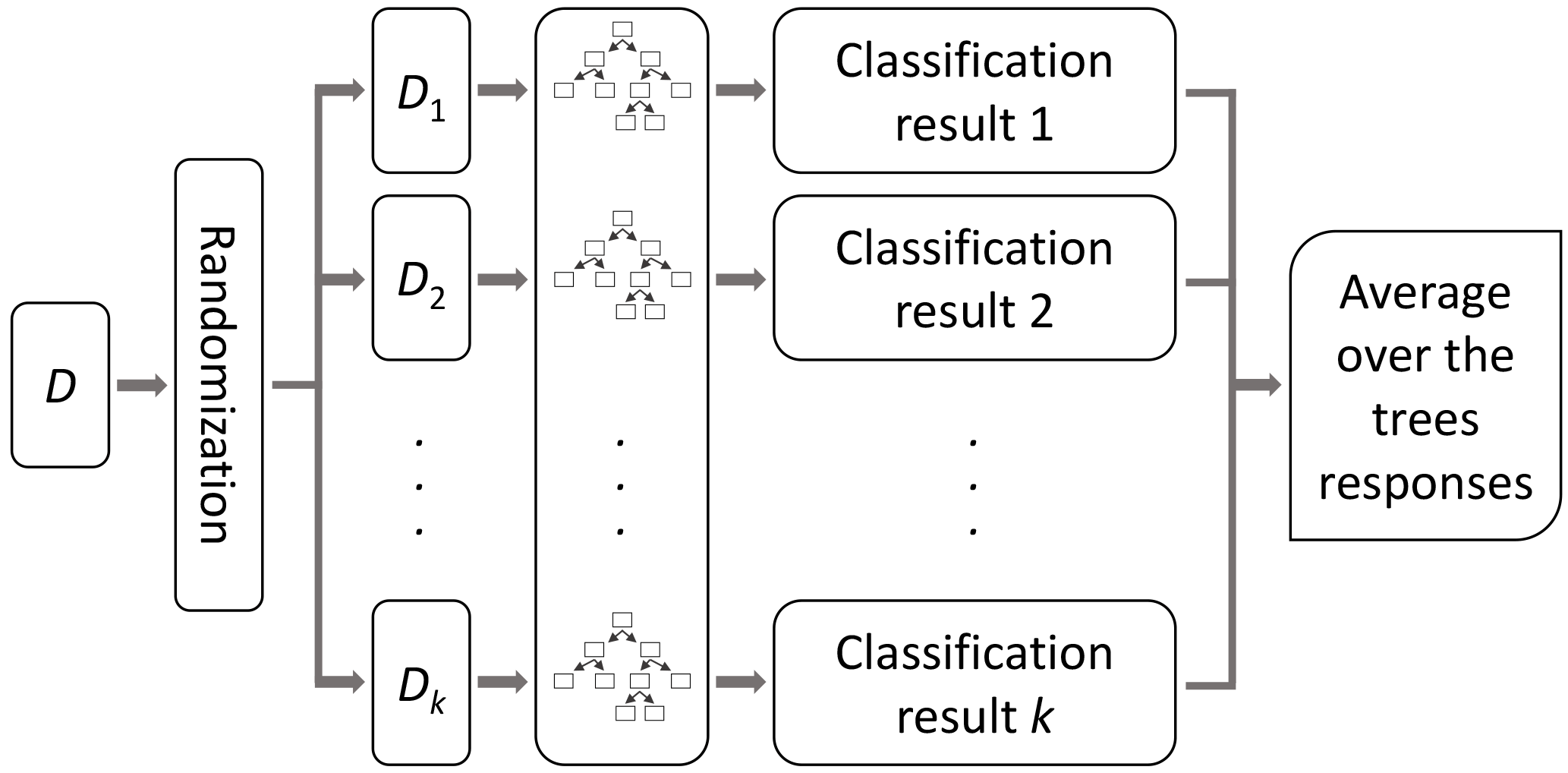
Figure 4Random forest method (Wang et al., 2015). An example of a regression tree built for the Secchia case study is shown in the Appendix (see Fig. B1).
The RF algorithm is used in many different scientific fields, from flood hazard assessment (Wang et al., 2015) to computer-aided diagnosis (Mihailescu et al., 2013), passing through gene selection (Deng and Runge, 2013), earthquake-induced damage classification (Solomon and Liu, 2010) and many others. The numerous applications show the many advantages of using the RF method, including high prediction accuracy, acceptable tolerance of outliers and noise, and easy avoidance of overfitting problems. In the last years, some applications of this method to flood risk have been performed (see Merz et al., 2013; Chinh et al., 2016; Hasanzadeh Nafari et al., 2016, 2017; Kreibich et al., 2017; Spekkers et al., 2014), but literature in this field is still scarce if compared to the numerous studies that use simpler univariable models. Nevertheless, Merz et al. (2013) demonstrated that tree-based models are able to improve the performance of existing models like stage-damage functions and to better identify the most informative independent variables and their interactions (e.g., they can identify different importance levels of the same variable, depending on the value of another variable).
Another important advantage of this algorithm is that no assumptions about independence, distribution or residual characteristics are needed. Further, RF allows the inclusion of both continuous, e.g., water depth or velocity, and categorical variables, e.g., building type. Conversely, multivariable models need a sufficient number of data in order to correctly identify complex relationships among variables. This is one of the reasons why this kind of model is scarcely used in regions where comprehensive, multidimensional databases are not available (Merz et al., 2013).
For RF learning, we consider all the variables that are available, collected from authorities, simulated by means of the hydrodynamic model and retrieved from external sources: maximum water depth, maximum water velocity, flood duration, building area, economic building value per unit area and building structural typology.
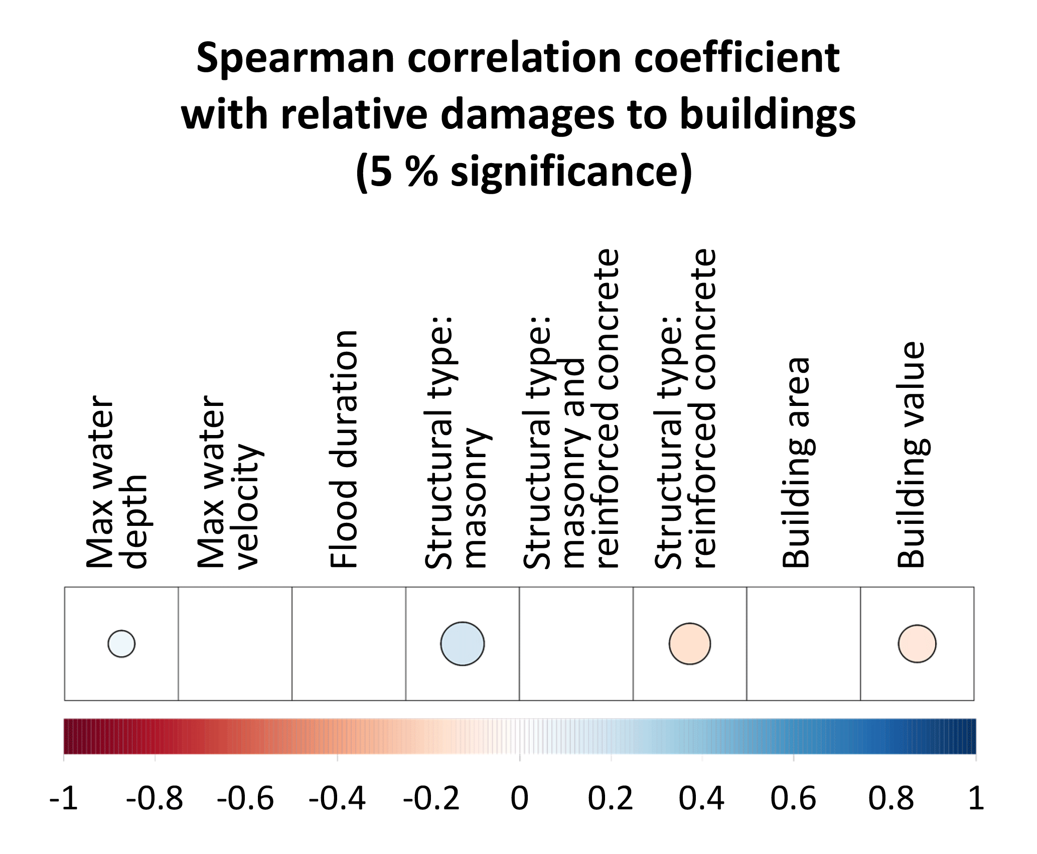
Figure 5Spearman correlation between relative loss (buildings only) and predictive variables: maximum water depth, maximum water velocity, flood duration, structural type (masonry, masonry and reinforced concrete, or reinforced concrete), building area and building value per unit area. Empty boxes indicate statistically nonsignificant correlation coefficients at a 5 % significance level.
5.1 Comparison of literature and empirical damage models
Figure 5 shows the results of the correlation analysis between relative flood loss to buildings and the available six predictive variables: maximum water depth, maximum water velocity, flood duration, building value per unit area, building area and building structural typology. Since the latter is a categorical variable, it is converted to dummy variable encoding in order to calculate the correlation of continuous and categorical data together. We refer to the Spearman correlation coefficient in order to also take into account nonlinear relationships among variables. Empty boxes represent correlations that are not statistically significant at a 5 % significance level. The variables that are significantly correlated with the relative loss to buildings are maximum water depth, building value per unit area and building structural typology. However, correlation coefficients are low, precisely lower than ±0.18 in all the cases. Similar results were obtained in terms of Pearson's correlation, but the values are not shown for the sake of brevity.
Figure 6 shows the output of the RF evaluation of the importance of the six predictive variables within the SMV model. This concept is different from the correlation one: in fact, while the Spearman coefficient indicates how well the relationship between two variables can be described using a monotonic function, the RF algorithm evaluates the importance of a variable by assessing the worsening in the performance of the model when that specific variable is not included in the database. In contrast to other studies (see, e.g., Merz et al., 2013), the dataset does not reveal a distinct importance for individual variables; not even water depth stands out. The descriptive capability of water depth is only slightly stronger than water velocity and building area, while the remaining predictors show very little importance.
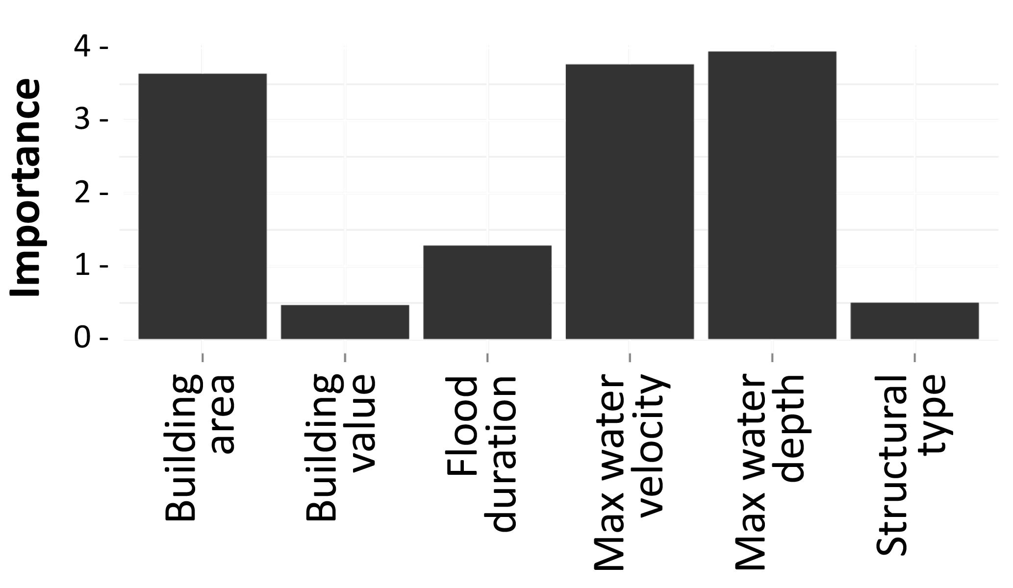
Figure 6Importance of predictive variables considered in SMV (building area, building value per unit area, flood duration, maximum water velocity, maximum water depth, structural type).
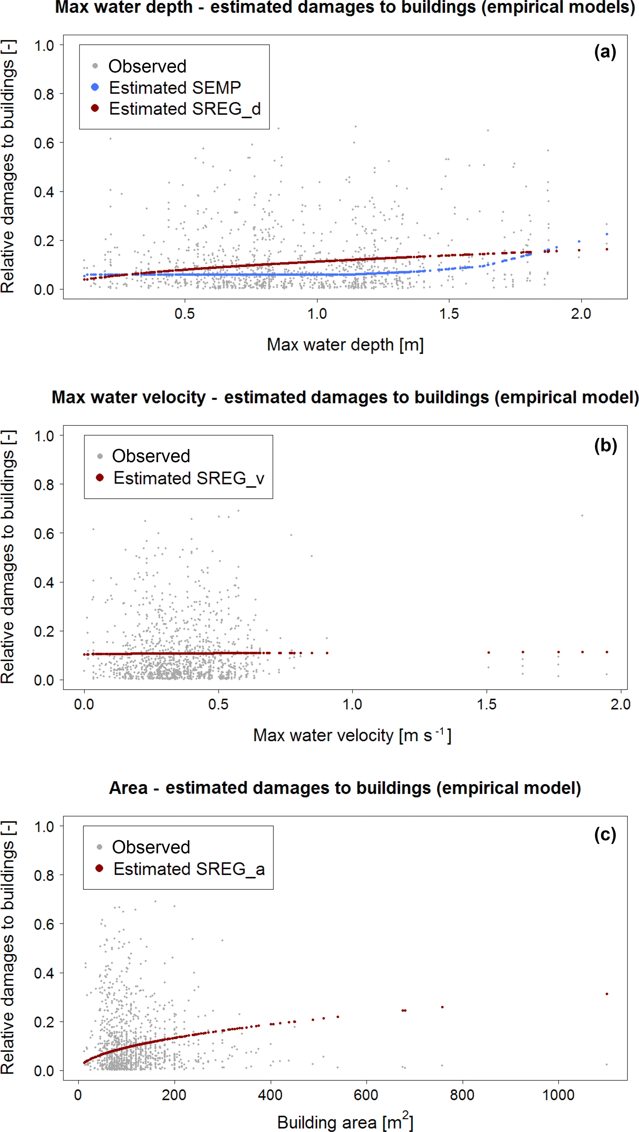
Figure 7Relative damages to buildings estimated with (a) SEMP (blue dots) and SREGd (dark red dots), (b) SREGv (dark red dots), and (c) SREGa (dark red dots). Grey points in the background represent observed relative loss to buildings.
Figure 7 shows in the background the observed relative damage to buildings, collected in the three affected municipalities (i.e., Bastiglia, Bomporto and Modena) as a function of maximum water depth (Fig. 7a), water velocity (Fig. 7b) and building area (Fig. 7c). Despite the statistically significant correlation with water depth (see Fig. 5), a very large noise can be observed in all diagrams, which implies that one variable alone explains only a very limited part of the damage process. This is confirmed from the outcomes of both the correlation assessment (see Fig. 5) and the importance analysis (see Fig. 6).
Taking the maximum water depth as the only explanatory variable, Fig. 7a represents the damages to buildings estimated by means of the univariable models developed based on the Secchia dataset (SEMP, with blue dots, and SREG_d, dark red dots). In a similar fashion, Fig. 7b, c show the relative loss to buildings as a function of maximum water velocity and building area, estimated by means of SREGv and SREGa, respectively (dark red dots in both diagrams).
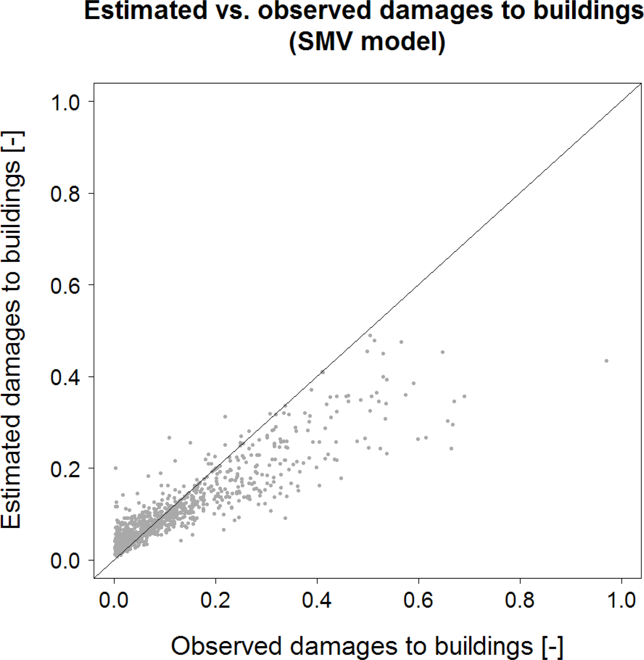
Results of the application of the multivariable model (SMV), described in Sect. 4.2.3, are shown in Fig. 8, which highlights the good performance of this model.
Table 4 quantifies the discrepancy between observed and predicted loss values for local empirical models in terms of four different performance metrics, namely bias, mean absolute error (MAE), RMSE and the difference between estimated and observed overall monetary loss to buildings (ΔLOSS), which are defined as follows:
in which Oi and Pi are observed and predicted relative damages at the ith site, respectively; n is the number of sites in the study area; and BAi and BVi are building area and building value per unit area at the ith site, respectively (see Table 3).
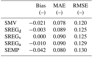
Table 4Performance of the uni- and multivariable models developed based on local data in estimating relative damages and overall monetary loss to buildings (see Eqs. 4, 5, 6 and 7; the observed overall monetary loss is equal to EUR 15.2 million). Models are ranked according to RMSE values, from the lowest to the largest. Corresponding results for literature models are reported in Table 5.
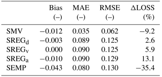
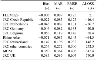
Table 5Performance of different literature univariable models in estimating relative damages and overall monetary loss to buildings (see Eqs. 4, 5, 6 and 7; the observed overall monetary loss is equal to EUR 15.2 million). Models are ranked according to RMSE values, from the lowest to the largest. Corresponding results for uni- and multivariable models developed based on local data are reported in Table 4.
SMV is associated with the lowest RMSE value (i.e., 0.062), which is less than half the RMSE value of the second-to-best models (i.e., SREGd and SREGv, with an RMSE value of 0.125). SREGa and SEMP provide slightly worse relative loss estimations than the previous models (RMSE equal to 0.129 and 0.130, respectively). Results are similar in terms of bias and MAE, although some differences can be pointed out for SREGx models, which present a bias value that is slightly lower than the one derived from SMV estimation.
Concerning literature models described in Sect. 4.1 and illustrated in Fig. 3, Table 5 shows that FLEMOps and JRC Czech Republic outperform the others in terms of RMSE (RMSE equal to 0.125 and 0.127, respectively) and are comparable with the models developed based on Secchia's dataset. RMSE values derived from the relative loss estimation with JRC Netherland, JRC Germany, JRC Belgium and Rhine Atlas are between 0.131 and 0.143, while the worst performance in terms of RMSE is associated with JRC Switzerland, JRC other countries, MCM and JRC UK (RMSE values higher than 0.2). These outcomes reflect the fact that all these latter damage curves are in the upper part of the diagram in Fig. 3 and significantly apart from the rest of the models, which are instead close to each other. We obtained similar results in terms of bias and MAE.
Analogous results can be observed in terms of ΔLOSS, which is reported in the rightmost column of both Tables 4 and 5. This indicator, different from MAE and RMSE and similar to bias, highlights the tendency of models to under- or overpredict damages to buildings; yet ΔLOSS focuses on the overall monetary damage in a given area, whereas bias refers to relative damages. Hence, ΔLOSS clearly shows if a model is biased in predicting the overall monetary loss, that is, if the model systematically predicts higher or lower (positive and negative bias, respectively) damages for the entire study area than those observed. This is shown in Fig. 8, in which most of the predictions provided by SMV, especially for observed relative damages higher than 10 %, lie under the 1:1 line: this means that the model is negatively biased. Predictions obtained with the other models are spread more evenly around the 1:1 line, denoting a smaller bias. In terms of bias and ΔLOSS, SMV seems to have a slightly worse performance than SREGd, SREGv and SREGa (and FLEMOps, regarding these specific outcomes).
The large overestimation of overall losses associated with JRC UK, MCM, JRC other countries, JRC Switzerland and JRC Belgium reported in Table 5 is expected from the comparison among these models and empirical data presented in Fig. 3. The overestimation may result from morphologic and socioeconomic contexts for which these models were constructed, as well as criteria adopted for their development, which might differ considerably from our case study and empirical models. For example, due to the diverse study area topographies and land uses, floods can propagate with various dynamics, differently influencing hazard indicators. Also, building characteristics and the overall well-being of an area can differ considerably among regions and countries, therefore compromising the transferability of literature curves.
Another feature of the rightmost column of Table 5 worth noting is that four of the literature models that perform the best in terms of RMSE (JRC Czech Republic, JRC Netherlands, JRC Germany and Rhine Atlas) underestimate the overall monetary loss. This fact can be explained by several reasons, among which an important one is certainly comparing damages claimed by citizens with the four models listed above, which were developed on the basis of expert-based judgment only, or by considering expert knowledge together with empirical data.
Table 6Validation of the models: performance of the uni- and multivariable models in estimating relative damages to buildings, developed based on two-thirds and validated based on the remaining one-third of the local data. Models are listed as in Table 4.
An additional important factor that influences the performance of literature models applied to the Secchia case study is the different scale on which these curves are calibrated and applied: some of them are developed to be applied at the microscale (e.g., MCM, FLEMOps), while others are developed to be applied at the mesoscale (e.g., Rhine Atlas, JRC curves). However, among mesoscale models there is a large variability in terms of performance. In several practical applications, identifying the best performing damage model a priori can be an extremely difficult task. This is also complicated by difficulties in obtaining detailed information about original datasets used for developing literature models (including damage data and characteristics of the flood event and of typology of affected buildings). Deeper investigation on model properties and assumptions (e.g., hazard and vulnerability features based on the context for which they have been derived, values used for translating monetary damage into relative damage, level of aggregation of original data) can guide the selection of models; moreover, a variety of them should be used to additionally obtain information on associated uncertainty (Figueiredo et al., 2018).
5.2 Validation of locally derived damage models
The results reported in Table 4 refer to calibrations of empirical models based on our entire dataset. We also validate all empirical models by using a split-sample validation procedure. Specifically, two-thirds of the records are randomly selected from the dataset for calibrating each model, which is then applied to the remaining one-third of the data. Bias, MAE and RMSE calculated in this context and reported in Table 6 are very similar to the ones reported in Table 4 concerning SREGx and SEMP. Results of the validation of SMV by means of the same approach instead indicate lower performance of this model, when calibrated on a smaller dataset (see Table 6). In fact, values of bias, MAE and RMSE are twice as high as values reported in Table 4. These outcomes highlight the need for extensive datasets for identifying robust and reliable damage models. From the comparison of the different considered models (uni- and multivariable), it is clear that this aspect is more evident for the multivariable model, whose performance is significantly worse when calibrated on a smaller number of observed data. Conversely, univariable models, though simpler than SMV, appear more robust in the case of a smaller number of calibration data, providing better results in the validation.
Based on the output of Sect. 5.1, it is worth noting that the application to the Secchia case study of JRC other countries, in which Italy should be included, provides very poor results in terms of building loss. This confirms how challenging the identification of a regional or large-scale model with a general validity could be (see also Sect. 1 and Cammerer et al., 2013; Amadio et al., 2016; Molinari et al., 2012). This section further assesses the transferability of damage models to very similar socioeconomic contexts.
In order to test the transferability of the empirical locally derived models to similar contexts, we identify analogous models (SREGx, since it is the best model among the locally derived ones, and SMV) on the basis of the building loss data collected in a single municipality and then apply these models for predicting flood building loss in a neighboring municipality. In particular, among the three municipalities considered in the study (i.e., Bomporto, Bastiglia and Modena), we consider Bastiglia (887 observed records) and Bomporto (392 observed records) because of the larger number of data available. We calibrate the models on Bomporto's subset (Bo_MV, Bo_REGd, Bo_REGv and Bo_REGa) and we apply them for predicting Bastiglia's flood damages to buildings. Then, we calibrate the same models on the Bastiglia subset (Ba_MV, Ba_REGd, Ba_REGv and Ba_REGa) and apply them to Bomporto.
Figure 9 shows the results of these split-sampling experiments. Figure 9a refers to Bastiglia's relative damages to buildings, estimated via Bo_MV and Bo_REGd, while Fig. 9b indicates Bomporto's damages estimated via Ba_MV and Ba_REGd; in each graph grey dots represent the estimation of relative loss using the multivariable models and red dots indicate relative damages to buildings estimated with square root regression models.

Figure 9(a) Bastiglia relative damages to buildings estimated with Bo_REGd (red dots) and Bo_MV (grey dots); (b) Bomporto relative damages to buildings estimated with Ba_REGd (red dots) and Ba_MV (grey dots).
Square root regression models in Fig. 9 show rather poor performances, capable of capturing only the average loss, while better results seem to be associated with multivariable models in both graphs. Some differences between the two panels are worth noting: grey dots in Fig. 9a (application of models calibrated in Bomporto with 392 data to Bastiglia) seem to overestimate relative loss to buildings, while in Fig. 9b (application of models calibrated in Bastiglia with 887 records to Bomporto) they lie closer to the 1:1 line. The studies performed in terms of relative damages to buildings related to maximum water velocity and building area present very similar results and are reported in the Appendix (see Figs. C1 and C2).
These outcomes are also visible in Table 7, which presents the results of the split-sampling experiments in terms of the usual bias, MAE and RMSE indexes. While uni- and multivariable models calibrated on Bastiglia's data and applied to Bomporto's subset do not differ much, with slightly better performances for Ba_MV, Bo_MV is associated with much higher prediction errors when applied to Bastiglia. The worse performance of Bo_MV can be explained by the smaller size of the Bomporto subset of data used for its calibration (less than a half of Bastiglia's sample). As already outlined in Sect. 4.2.3, in order to have robust results from multivariable models, a large number of empirical data are required. Furthermore, the inundated area in Bomporto is larger than in Bastiglia (see Fig. 2). This explains rather clearly the difference in terms of accuracy of Ba_MV and Bo_MV in Table 7: the higher the loss data density the more robust the relationship between different predictor variables and loss data and the higher the ability of the model to explain local characteristics of the study area (Schröter et al., 2014).
Table 7Transferability of the models: performance of different uni- and multivariable models in estimating relative damages to buildings in different contexts. In the upper tables, the models were calibrated on Bomporto's dataset (392 records) and validated in Bastiglia, while in the bottom tables the models were calibrated on Bastiglia's dataset (887 records) and used to estimate damages in Bomporto. The left tables report performance of the models in the calibration phase, while the right tables show performance of the validation study.
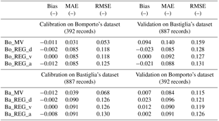
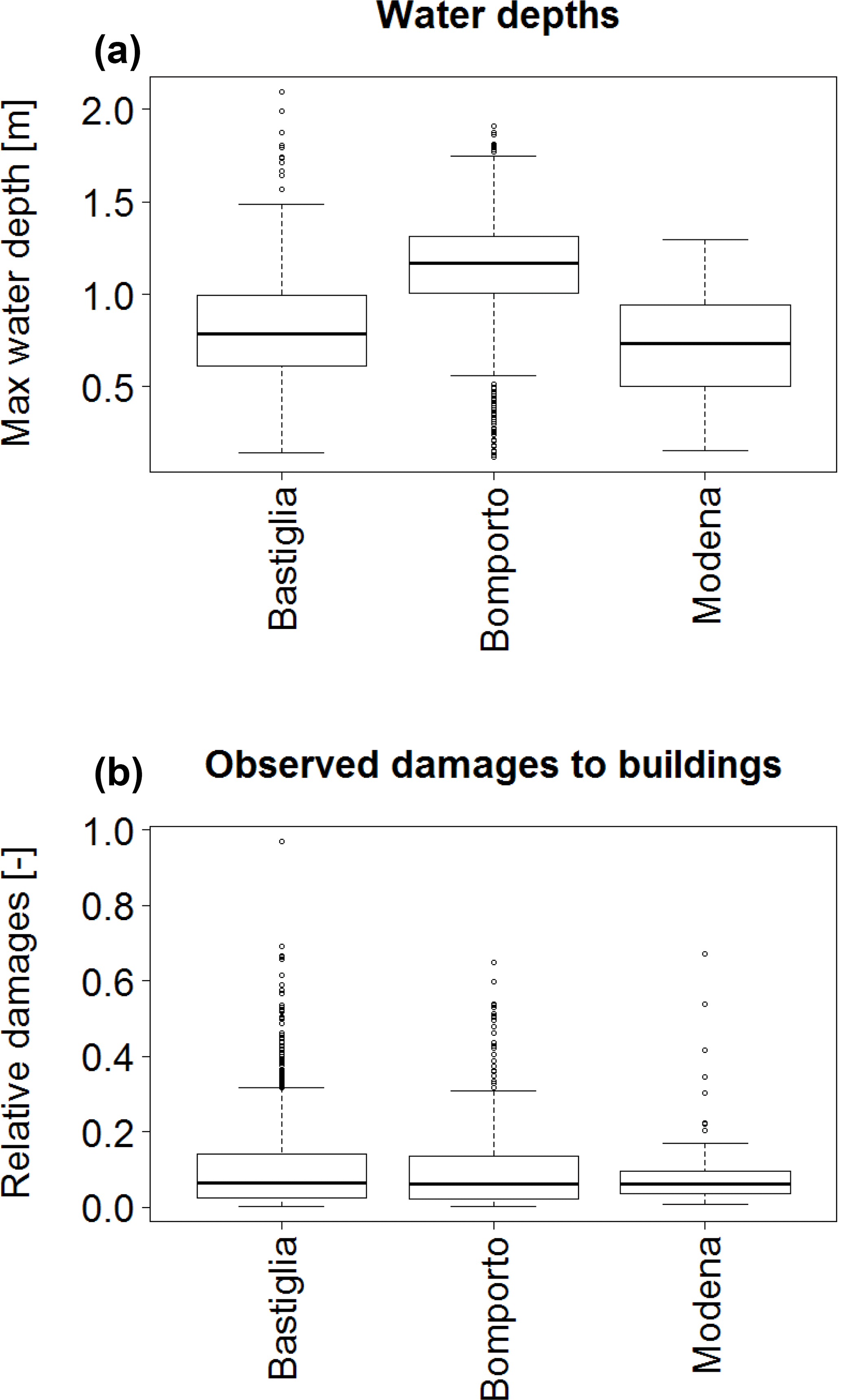
Figure 10Distribution of water depths (a) and observed relative damages (b) in the three considered municipalities.
The transferability of the models is also hampered by the different distribution of the water depths in the different municipalities: Fig. 10 shows that water depths in Bastiglia are lower than in Bomporto, despite the quite similar distribution of observed relative damages. This might be due to the fact that, other than being a hazard, different buildings' vulnerability plays an important role in the damage process too and it also explains prediction errors in the analysis. This aspect has to be taken into consideration whenever the loss estimation is performed by using a model calibrated for a different flood event.
5.3 Modeling flood loss to contents
Similar to the procedure for assessing damages to buildings, first of all we analyze the Spearman correlation between the observed flood loss to contents and all potential predictive variables, included monetary damages to buildings. Figure 11 shows the results of this assessment, where full boxes represent a statistically significant correlation coefficient at a 5 % significance level. On the one hand, similar to the analysis for building loss, the maximum water depth and the structural typology are significantly correlated with damages to contents, although their correlation coefficients are low. On the other hand, damages to contents turn out to be significantly correlated with the building footprint (Spearman correlation coefficient equal to 0.27) instead of the building value. A noteworthy feature of Fig. 11 is the very strong and statistically significant positive correlation between damages to buildings and their contents (Spearman correlation coefficient equal to 0.59).
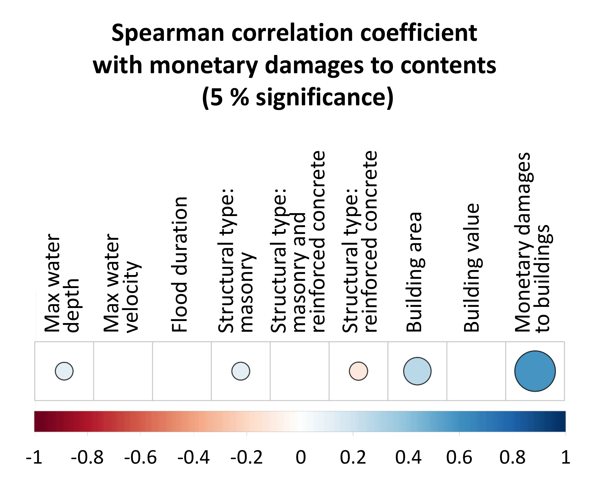
Figure 11Spearman correlation between monetary loss (contents only) and predictive variables: maximum water depth, maximum water velocity, flood duration, structural type (masonry, masonry and reinforced concrete, or reinforced concrete), building area, building value per unit area and monetary loss to buildings. Empty boxes indicate statistically nonsignificant correlation coefficients at a 5 % significance level.
We therefore explore the possibility of exploiting the relationship between monetary loss to buildings and contents for predicting the latter. We test different types of mathematical relationships (i.e., linear, square root, logarithmic and bi-logarithmic regressions), and the square root regression is the one with the best prediction performance in terms of RMSE, i.e., the one that best relates monetary building loss with damages to contents. In fact, RMSE is equal to EUR 10 569, while it was EUR 10 882, 10 971 and 15 531 for linear, logarithmic and bi-logarithmic relationships, respectively. The identified regression relationship reads
where Dcontents (EUR) represents economic damages to contents, and Dbuildings (EUR) indicates loss to buildings. Figure 12 depicts empirical vs. predicted monetary loss to contents with Eq. (8).
Table 8Performance of different uni- and multivariable models in estimating relative damages and overall monetary loss to contents (see Eqs. 4, 5, 6 and 7; the observed overall monetary loss is equal to EUR 10.4 million). The first row shows the performance of Eq. (8) applied to the observed monetary damages to buildings; the first block represents the results of the application of Eq. (8) to monetary building damages estimated with locally derived models, while the second represents those estimated with literature models. Models in each group are ranked according to RMSE values, from the lowest to the largest.
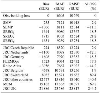
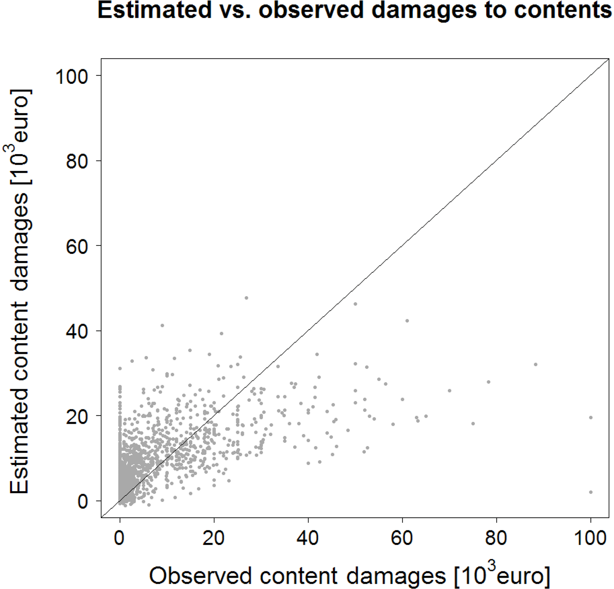
Figure 12Empirical vs. predicted monetary loss to contents for the Secchia 2014 inundation event. Monetary loss to contents is predicted as a function of monetary loss to buildings through Eq. (8).
In the last component of our analysis, we apply Eq. (8) for estimating damages to contents as a function of the estimates of monetary building loss resulting from the uni- and multivariable damage models that we considered in our study.
Table 8 lists the performance metrics bias, MAE, RMSE and ΔLOSS obtained while predicting monetary loss to contents as described. The first row in Table 8 reports, as a reference term, the same performance indexes that can be obtained when Eq. (8) is applied to observed damages to buildings. In the second row, the first block of Table 8 shows the performance in estimating monetary content loss, applying Eq. (8) to monetary damages to buildings, estimated with empirically derived models. The best performance in terms of RMSE is always associated with SMV, followed by SEMP and SREGx, all with comparable RMSE values. The outcomes for literature models (last block of Table 8) also reflect the results that we obtained when modeling building loss, presented in Sect. 5.1. The ranking of the best-performing literature models in terms of RMSE for an indirect assessment of content loss is JRC Czech Republic, JRC Netherlands, JRC Germany, FLEMOps, Rhine Atlas and JRC Belgium. Evidently, models associated with poor performances in predicting monetary loss to buildings are also not reliable for indirectly predicting loss to building contents by means of Eq. (8) (see JRC Switzerland, JRC other countries, MCM and JRC UK). The performance of most considered models, with the exception of the last six in Table 8, show a difference between overall observed and predicted monetary loss to contents that does not exceed EUR ±20 million. Different from the results obtained when predicting damages to buildings, 11 damage models overestimate content loss, while SEMP, JRC Netherlands, JRC Germany and Rhine Atlas underestimate them. Small differences in the models' ranking, compared to Tables 4 and 5, are probably due to the fact that the regression curve for content damages is applied to predicted building damages, which are themselves affected by uncertainty.
Our study focuses on the development and validation of flood loss models based on a comprehensive database of observed loss data (1330 records), collected after a recent inundation event in Italy. We derived empirical uni- and multivariable damage models, whose performance has been compared with that of stage-damage functions in the literature (MCM, FLEMOps, Rhine Atlas and JRC models for different countries).
Consistent with the findings of Cammerer et al. (2013), Dottori et al. (2016a), and Scorzini and Frank (2015), locally identified empirical models provide better estimation of relative and monetary damages to buildings. This result underlines the criticality and uncertainty associated with the application of literature damage models to different contexts from the ones in which they were originally developed. Even though some literature models have performance similar to locally identified empirical models, the difficulty to retrieve detailed information about their development data and procedures makes it difficult to identify a priori the best-performing literature models. This hampers the practical utilization of literature models themselves for predictive purposes. The results of this study strengthen the need, in case a literature curve should be applied, for a more informed and rational selection of damage models; e.g., the level of detail of each input variable required should not be overlooked nor neglected.
Concerning the estimation of relative loss to buildings, the Secchia Multi-Variable model (SMV), which was developed using the RF approach, outperforms the other considered models. This outcome is confirmed with regards to the content damages, estimated with a regression function applied to the monetary damages to buildings estimated with different models. Regression trees composing the multivariable forest also provide the important advantage of avoiding the need for a parametric function that works with all the data. Also, RF provides useful information about the relationship among the variables and how to exploit the local relevance of predictors. These can be very useful information for authorities and stakeholders to define preventive measures and/or mitigation strategies.
The study on the transferability of empirical models, i.e., models calibrated on the dataset of one given municipality and applied to a different one located close by, shows that the best performance is controlled by the size and consistency of the loss dataset. This consideration is valid for all models, but especially for the multivariable one, which requires a large number of data to ensure a reliable loss estimation (Merz et al., 2013; Schröter et al., 2014). To completely exploit the potential of such models and sustain the possibility of exporting their use in different areas, it is necessary to pursue a detailed and structured acquisition of explanatory variables. According to Amadio et al. (2016), Molinari et al. (2012, 2014b), and Scorzini and Frank (2015), the most urgent need in Italy, concerning flood loss estimation, is to identify guidelines, valid for the whole country, to collect consistent and comparable data, even if they relate to different contexts. According to Ballio et al. (2015), data-collection protocols are urgently needed for harmonizing and standardizing the compilation of flood loss datasets. These data should include further useful information, such as observed water depths, flood duration, presence of sediments, contamination rate, early warning or precautionary measures adopted, and other indications of the building composition (numbers of floors, type of contents, presence of basements, building condition, etc.), preferably collected immediately post event (see also Merz et al., 2010), in addition to that commonly collected.
As it emerges from our analysis, in the case of limited and uncertain information, empirically univariable models still represent a good compromise between model complexity and reliable damage estimations. Different from other studies, which developed site-specific models but rarely tested them in other regions, this analysis focuses on transferability and demonstrates that models can be transferred to other contexts with satisfying results, provided that they are similar in terms of territorial structure and building characteristics. Since the creation of a “one-size-fits-all” model is almost impossible due to large variability in geographical and geomorphological contexts as well as urban patterns and building typologies in Italy, the definition of various damage models for different standardized Italian contexts is of paramount importance to increase the reliability of future flood risk analyses. The adoption of probabilistic modeling concepts could add another useful level of detail in terms of quantitative information about the uncertainty.
Damage data used in this study, as well as building characteristics, provided by the Emilia-Romagna Region Regional Agency for Civil Protection and Po River Basin Authority, are not publicly accessible for privacy reasons. Economic building values can be found at https://wwwt.agenziaentrate.gov.it/servizi/Consultazione/ricerca.htm (Agenzia delle Entrate, 2018).
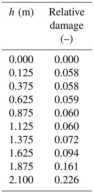
SEMP is the linear interpolation of points with specific coordinates, calculated as explained in Sect. 4.2.1. These coordinates are reported in Table A1.
Table A1SEMP model: empirical curve obtained from the binning procedure in terms of water depth (h) and relative damage to buildings (see Sect. 4.2.1 for the procedure adopted to develop the curve).
SMV is an ensemble of several regression trees, built from the bootstrap replica of the learning data, as explained in Sect. 4.2.3. Figure B1 reports a qualitative example of one of these regression trees for the Secchia case study, cut off at an arbitrary level for the sake of clarity.

Figure B1Example of a tree built with the RF algorithm on the basis of the Secchia dataset. White boxes represent splitting nodes, together with the indication of the splitting variable and its splitting value; grey boxes represent final nodes and the estimation of the relative building damages of that branch. The tree is cut off at an arbitrary level for the sake of clarity.
Figures C1 and C2 show the results of the validation of the locally derived models, which estimate relative damages to buildings as a function of maximum water velocity and building area.
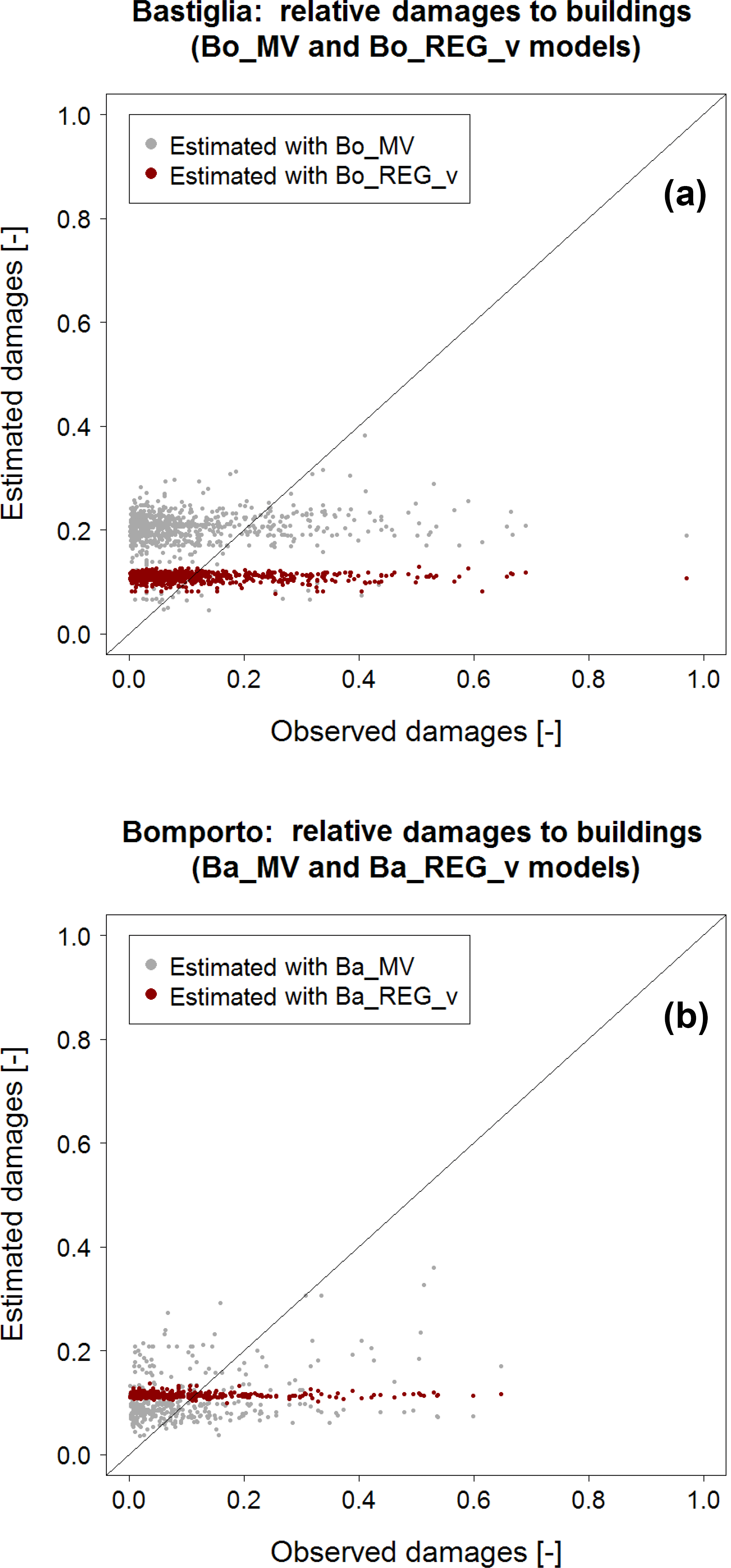
Figure C1(a) Bastiglia relative damages to buildings estimated with Bo_REGv (red dots) and Bo_MV (grey dots); (b) Bomporto relative damages to buildings estimated with Ba_REGv (red dots) and Ba_MV (grey dots).
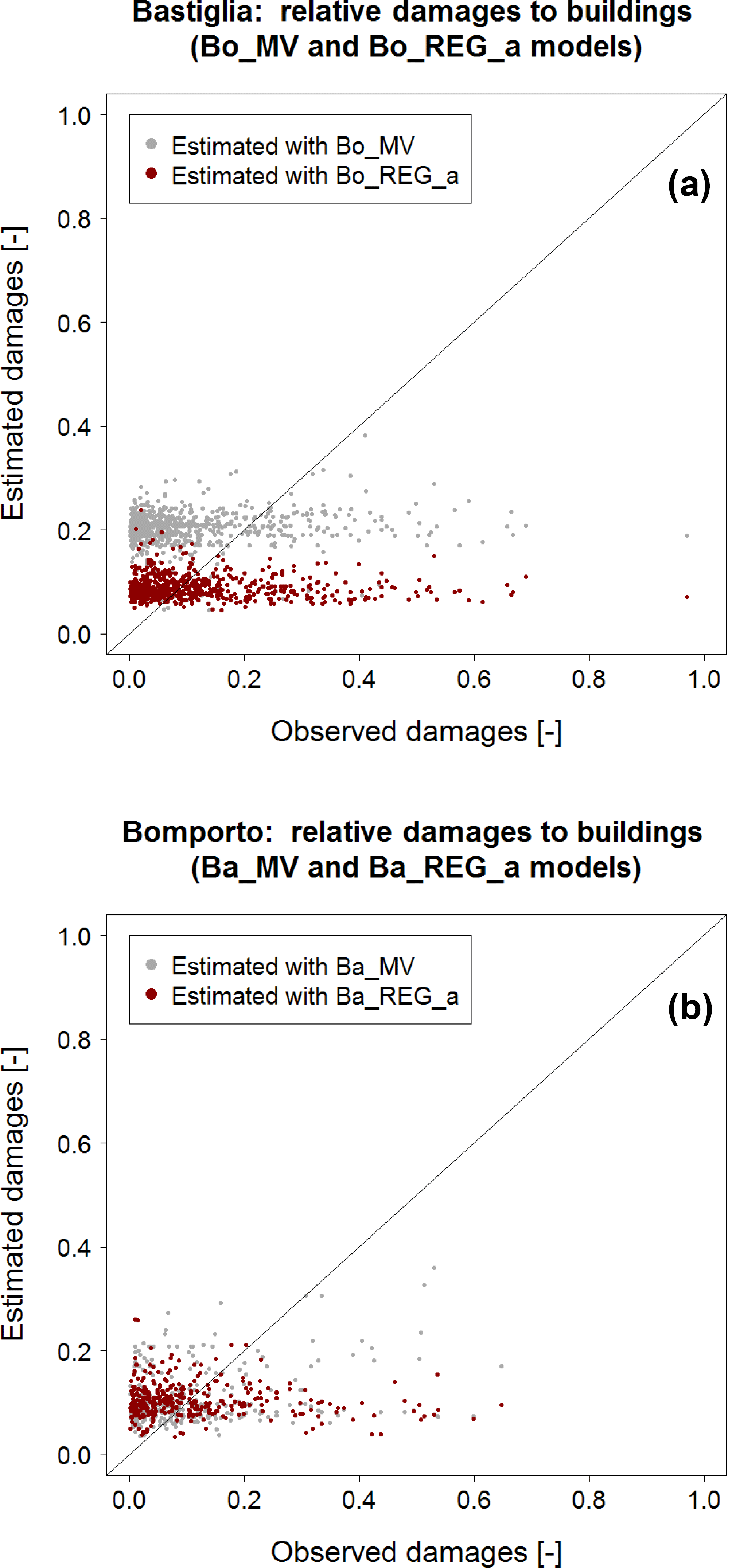
Figure C2(a) Bastiglia relative damages to buildings estimated with Bo_REGa (red dots) and Bo_MV (grey dots); (b) Bomporto relative damages to buildings estimated with Ba_REGa (red dots) and Ba_MV (grey dots).
The original dataset was checked, homogenized and geocoded by FC, who also performed the numerical analyses, within the activities of her PhD thesis. KS and HK had an essential role in the development of the multivariable model while AD and AC contributed to the development and testing of the empirical univariable ones. All authors made a substantial contribution to the critical interpretation of results and provided important ideas to further improve the study. All authors actively took part in drafting, writing and revising the paper.
The authors declare that they have no conflict of interest.
The Emilia-Romagna region, Regional Agency for Civil Protection and Po River
Basin Authority are kindly acknowledged for providing the datasets used in
this study. In fact, part of the activity was performed with the support and
contribution of the Civil Protection Agency of Emilia-Romagna under a
5-year framework research agreement with the Department of Civil,
Chemical, Environmental and Materials Engineering (DICAM) of the University
of Bologna (DICAM-PCREM, 2015). The present work was also developed
within the framework of the Panta Rhei Research Initiative of the
International Association of Hydrological Sciences (IAHS). Funding was partly
provided by the University of Bologna, the SYSTEM-RISK
Marie Skłodowska-Curie European Training Network (EU grant 676027) and the
IMPREX project (EU grant 641811). Finally, the authors would like to
sincerely thank the two anonymous reviewers for their effort to improve the
paper with valuable comments and suggestions.
Edited by: Margreth Keiler
Reviewed by: two anonymous referees
Agenzia delle Entrate: Banca dati delle quotazioni immobiliari (Real estate quotation database), https://wwwt.agenziaentrate.gov.it/servizi/Consultazione/ricerca.htm, last access: July 2018. a
Amadio, M., Mysiak, J., Carrera, L., and Koks, E.: Improving flood damage assessment models in Italy, Nat. Hazards, 82, 2075–2088, https://doi.org/10.1007/s11069-016-2286-0, 2016. a, b, c, d, e, f
Apel, H., Aronica, G. T., Kreibich, H., and Thieken, A. H.: Flood risk analyses – How detailed do we need to be?, Nat. Hazards, 49, 79–98, https://doi.org/10.1007/s11069-008-9277-8, 2009. a, b, c
Arrighi, C., Brugioni, M., Castelli, F., Franceschini, S., and Mazzanti, B.: Urban micro-scale flood risk estimation with parsimonious hydraulic modelling and census data, Nat. Hazards Earth Syst. Sci., 13, 1375–1391, https://doi.org/10.5194/nhess-13-1375-2013, 2013. a
Ballio, F., Molinari, D., Minucci, G., Mazuran, M., Arias Munoz, C., Menoni, S., Atun, F., Ardagna, D., Berni, N., and Pandolfo, C.: The RISPOSTA procedure for the collection, storage and analysis of high quality, consistent and reliable damage data in the aftermath of floods, J. Flood Risk Manage., 11, S604–S615, https://doi.org/10.1111/jfr3.12216, 2015. a, b
Barredo, J. I.: Normalised flood losses in Europe: 1970–2006, Nat. Hazards Earth Syst. Sci., 9, 97–104, https://doi.org/10.5194/nhess-9-97-2009, 2009. a
Breiman, L.: Random forests, Mach. Learn., 45, 5–32, https://doi.org/10.1023/A:1010933404324, 2001. a
Breiman, L., Friedman, J., Olshen, R. A., and Stone, C. J.: CART: Classification and Regression Trees, Wadsworth, Belmont, CA, 1984. a
Brière, C., Abadie, S., Bretel, P., and Lang, P.: Assessment of TELEMAC system performances, a hydrodynamic case study of Anglet, France, Coast. Eng., 54, 345–356, https://doi.org/10.1016/j.coastaleng.2006.10.006, 2007. a
Bubeck, P. and Kreibich, H.: Natural Hazards: direct costs and losses due to the disruption of production pro- esses – CONHAZ (Costs of Natural Hazards) Report, Tech. rep., CONHAZ Consortium, Potsdam, 2011. a, b, c, d
Bubeck, P., de Moel, H., Bouwer, L. M., and Aerts, J. C. J.: How reliable are projections of future flood damage?, Nat. Hazards Earth Syst. Sci., 11, 3293–3306, https://doi.org/10.5194/nhess-11-3293-2011, 2011. a
Büchele, B., Kreibich, H., Kron, A., Thieken, A., Ihringer, J., Oberle, P., Merz, B., and Nestmann, F.: Flood-risk mapping: Contributions towards an enhanced assessment of extreme events and associated risks, Nat. Hazards Earth Syst. Sci., 6, 483–503, https://doi.org/10.5194/nhess-6-485-2006, 2006. a
Cammerer, H., Thieken, A. H., and Lammel, J.: Adaptability and transferability of flood loss functions in residential areas, Natural Hazards Earth Syst. Sci., 13, 3063–3081, https://doi.org/10.5194/nhess-13-3063-2013, 2013. a, b, c, d, e
Carisi, F., Domeneghetti, A., Gaeta, M. G., and Castellarin, A.: Is anthropogenic land-subsidence a possible driver of riverine flood-hazard dynamics? A case study in Ravenna, Italy, Hydrolog. Sci. J., 62, 2440–2455, 2017. a
Castellarin, A., Di Baldassarre, G., Bates, P. D., and Brath, A.: Optimal Cross-Sectional Spacing in Preissmann Scheme 1D Hydrodynamic Models, J. Hydraul. Eng., 135, 96–105, https://doi.org/10.1061/(ASCE)0733-9429(2009)135:2(96), 2009. a
Chinh, D. T., Gain, A. K., Dung, N. V., Haase, D., and Kreibich, H.: Multi-variate analyses of flood loss in Can Tho city, Mekong delta, Water, 8, 1–21, https://doi.org/10.3390/w8010006, 2016. a, b
Ciscar, J.-C., Iglesias, A., Feyen, L., Szabó, L., Van Regemorter, D., Amelung, B., Nicholls, R., Watkiss, P., Christensen, O. B., Dankers, R., Garrote, L., Goodess, C. M., Hunt, A., Moreno, A., Richards, J., and Soria, A.: Physical and economic consequences of climate change in Europe, P. Natl. Acad. Sci. USA, 108, 2678–2683, 2011. a
D'Alpaos, L., Brath, A., Fioravante, V., Gottardi, G., Mignosa, P., and Orlandini, S.: Relazione tecnico-scientifica sulle cause del collasso dell' argine del fiume Secchia avvenuto il giorno 19 gennaio 2014 presso la frazione San Matteo, Tech. rep., Bologna, Italy, http://ambiente.regione.emilia-romagna.it/geologia/notizie/notizie-2014/fiume-secchia (last access: July 2018), 2014. a, b, c, d
de Moel, H. and Aerts, J. C. J. H.: Effect of uncertainty in land use, damage models and inundation depth on flood damage estimates, Nat. Hazards, 58, 407–425, https://doi.org/10.1007/s11069-010-9675-6, 2011. a
de Moel, H., Asselman, N. E. M., and Aerts, J. C. J.: Uncertainty and sensitivity analysis of coastal flood damage estimates in the west of the Netherlands, Nat. Hazards Earth Syst. Sci., 12, 1045–1058, https://doi.org/10.5194/nhess-12-1045-2012, 2012. a
de Moel, H., Bouwer, L. M., and Aerts, J. C. J. H.: Uncertainty and sensitivity of flood risk calculations for a dike ring in the south of the Netherlands, Sci. Total Environ., 473–474, 224–234, https://doi.org/10.1016/j.scitotenv.2013.12.015, 2014. a
de Moel, H., Jongman, B., Kreibich, H., Merz, B., Penning-Rowsell, E., and Ward, P. J.: Flood risk assessments at different spatial scales, Mitig. Adapt. Strat. Global Change, 20, 865–890, https://doi.org/10.1007/s11027-015-9654-z, 2015. a
Deng, H. and Runge, G.: Gene selection with guided regularized random forest, Pattern Recog., 46, 3483–3489, 2013. a
DICAM-PCREM: Convenzione-quadro quinquennale di ricerca tra Agenzia di Protezione Civile della Regione Emilia-Romagna e il Dipartimento di Ingegneria Civile, Chimica, Ambientale e dei Materiali ALMA MATER STUDIORUM, Relazione conclusiva quarta, Tech. rep., Università di Bologna, Bologna, 2015. a, b
Domeneghetti, A., Vorogushyn, S., Castellarin, A., Merz, B., and Brath, A.: Probabilistic flood hazard mapping: Effects of uncertain boundary conditions, Hydrol. Earth Syst. Sci., 17, 3127–3140, https://doi.org/10.5194/hess-17-3127-2013, 2013. a
Domeneghetti, A., Carisi, F., Castellarin, A., and Brath, A.: Evolution of Flood Risk Over Large Areas: Quantitative Assessment for The Po River, J. Hydrol., 527, 809–823, https://doi.org/10.1016/j.jhydrol.2015.05.043, 2015. a, b
Dottori, F., Figueiredo, R., Martina, M., Molinari, D., and Scorzini, A. R.: INSYDE: a synthetic, probabilistic flood damage model based on explicit cost analysis, Nat. Hazards Earth Syst. Sci., 16, 2577–2591, https://doi.org/10.5194/nhess-2016-163, 2016a. a, b
Dottori, F., Martina, M. L. V., and Figueiredo, R.: A methodology for flood susceptibility and vulnerability analysis in complex flood scenarios, J. Flood Risk Manage., 11, S632–S645, https://doi.org/10.1111/jfr3.12234, 2016b. a
European Environment Agency: CLC2006 technical guidelines, Tech. Rep. 17, Copenhagen, Denmark, https://doi.org/10.2800/12134, 2007. a, b
Feyen, L., Dankers, R., Bodis, K., Salamon, P., and Barredo, J. I.: Fluvial flood risk in Europe in present and future climates, Climate Change, 112, 47–62, https://doi.org/10.1007/s10584-011-0339-7, 2012. a
Figueiredo, R., Schröter, K., Weiss-Motz, A., Martina, M. L. V., and Kreibich, H.: Multi-model ensembles for assessment of flood losses and associated uncertainty, Nat. Hazards Earth Syst. Sci., 18, 1297–1314, https://doi.org/10.5194/nhess-18-1297-2018, 2018. a
Freni, G., La Loggia, G., and Notaro, V.: Uncertainty in urban flood damage assessment due to urban drainage modelling and depth-damage curve estimation, Water Sci. Technol., 61, 2979–2993, 2010. a
Galland, J. C., Goutal, N., and Hervouet, J. M.: Telemac: a new numerical model for solving shallow water equations, Adv. Water Resour., 14, 38–148, 1991. a
Gerl, T., Kreibich, H., Franco, G., Marechal, D., and Schröter, K.: A review of flood loss models as basis for harmonization and benchmarking, PLOS ONE, 11, 1–22, https://doi.org/10.1371/journal.pone.0159791, 2016. a, b, c, d
Green, C., Viavattene, C., Thompson, P., and Green, C.: Guidance for assessing flood losses – CONHAZ (Costs of Natural Hazards) Report, Tech. rep., Middlesex University, Middlesex, 2011. a, b
Guha-Sapir, D. and CRED: The human cost of natural disasters 2015 – A global perspective, Tech. rep., Centre for Research on the Epidemiology of Disasters (CRED), Brussels, Belgium, 2015. a
Guha-Sapir, D. and CRED: 2016 preliminary data: Human impact of natural disasters, Tech. Rep. 45, Centre for Research on the Epidemiology of Disasters (CRED), Brussels, Belgium, 2016. a
Hasanzadeh Nafari, R., Ngo, T., and Lehman, W.: Calibration and validation of FLFArs-A new flood loss function for Australian residential structures, Nat. Hazards Earth Syst. Sci., 16, 15–27, https://doi.org/10.5194/nhess-16-15-2016, 2016. a, b
Hasanzadeh Nafari, R., Amadio, M., Ngo, T., and Mysiak, J.: Flood loss modelling with FLF-IT: A new flood loss function for Italian residential structures, Nat. Hazards Earth Syst. Sci., 17, 1047–1059, https://doi.org/10.5194/nhess-17-1047-2017, 2017. a, b
Hervouet, J. M. and Bates, P.: The Telemac modelling system, special issue, Hydrol. Process., 14, 2207–2363, 2000. a, b
Huizinga, J.: Flood damage functions for EU member states, Technical report, HKV Consultants, Lelystad, Implemented in the framework of the contract # 382441-F1SC awarded by the European Commission – Joint Research Centre, 2007. a
IPCC: Climate Change 2001: Synthesis Report, Tech. rep., New York, NY, USA, 2001. a
IPCC: Climate Change 2014: Synthesis Report, Tech. rep., Geneva, Switzerland, https://doi.org/10.1017/CBO9781107415324, 2014. a, b
Jongman, B., Kreibich, H., Apel, H., Barredo, J. I., Bates, P. D., Feyen, L., Gericke, A., Neal, J., Aerts, J. C. J. H., and Ward, P. J.: Comparative flood damage model assessment: towards a European approach, Nat. Hazards Earth Syst. Sci., 12, 3733–3752, https://doi.org/10.5194/nhess-12-3733-2012, 2012. a, b, c, d, e, f, g, h, i
Kreibich, H., Piroth, K., Seifert, I., Maiwald, H., Kunert, U., Schwarz, J., Merz, B., and Thieken, A. H.: Is flow velocity a significant parameter in flood damage modelling?, Nat. Hazards Earth Syst. Sci., 9, 1679–1692, https://doi.org/10.5194/nhess-9-1679-2009, 2009. a
Kreibich, H., Seifert, I., Merz, B., and Thieken, A. H.: Development of FLEMOcs – a new model for the estimation of flood losses in the commercial sector, Hydrolog. Sci. J., 55, 1302–1314, https://doi.org/10.1080/02626667.2010.529815, 2010. a
Kreibich, H., Botto, A., Merz, B., and Schröter, K.:Probabilistic, Multivariable Flood Loss Modeling on the Mesoscale with BT-FLEMO, Risk Anal., 37, 774–787, https://doi.org/10.1111/risa.12650, 2017. a, b
Liaw, A. and Wiener, M.: Classification and Regression by randomForest, R News, 2, 18–22, http://CRAN.R-project.org/doc/Rnews/, 2002. a
Luino, F., Chiarle, M., Nigrelli, G., Agangi, A., Bidoccu, M., Cirio, C. G., and Giulietto, W.: A model for estimating flood damage in Italy: preliminary results, Environ. Econ. Invest. Assess., 98, 1–10, https://doi.org/10.2495/EEIA060071, 2006. a
Manciola, P., Biscarini, C., and Cingolani, A.: La mappatura delle aree inondabili, in: Proceedings of “Riqualificazione, Difesa Idraulica e Recupero Ambientale delle Sponde Fluviali”, 26–28 May 2003, Perugia, Italy, 2003. a
Merz, B., Kreibich, H., Thieken, A., and Schmidtke, R.: Estimation uncertainty of direct monetary flood damage to buildings, Nat. Hazards Earth Syst. Sci., 4, 153–163, https://doi.org/10.5194/nhess-4-153-2004, 2004. a, b, c
Merz, B., Thieken, A. H., and Gocht, M.: Flood Risk Mapping At The Local Scale: Concepts and Challenges, Springer Netherlands, Dordrecht, the Netherlands, 2007. a, b
Merz, B., Kreibich, H., Schwarze, R., and Thieken, A.: Review article “Assessment of economic flood damage”, Nat. Hazards Earth Syst. Sci., 10, 1697–1724, https://doi.org/10.5194/nhess-10-1697-2010, 2010. a, b, c, d, e
Merz, B., Kreibich, H., and Lall, U.: Multi-variate flood damage assessment: A tree-based data-mining approach, Nat. Hazards Earth Syst. Sci., 13, 53–64, https://doi.org/10.5194/nhess-13-53-2013, 2013. a, b, c, d, e, f, g, h, i, j, k, l, m, n
Merz, B., Aerts, J., Arnbjerg-Nielsen, K., Baldi, M., Becker, A., Bichet, A., Blöschl, G., Bouwer, L. M., Brauer, A., Cioffi, F., Delgado, J. M., Gocht, M., Guzzetti, F., Harrigan, S., Hirschboeck, K., Kilsby, C., Kron, W., Kwon, H. H., Lall, U., Merz, R., Nissen, K., Salvatti, P., Swierczynski, T., Ulbrich, U., Viglione, A., Ward, P. J., Weiler, M., Wilhelm, B., and Nied, M.: Floods and climate: Emerging perspectives for flood risk assessment and management, Nat. Hazards Earth Syst. Sci., 14, 1921–1942, https://doi.org/10.5194/nhess-14-1921-2014, 2014. a
Messner, F., Penning-Rowsell, E., Green, C., Meyer, V., Tunstall, S., and van der Veen, A.: Evaluating flood damages: guidance and recommendations on principles and methods, Tech. rep., HR Wallingford, Wallingford, UK, 2007. a, b
Meyer, V., Becker, N., Markantonis, V., Schwarze, R., Van Den Bergh, J. C. J. M., Bouwer, L. M., Bubeck, P., Ciavola, P., Genovese, E., Green, C., Hallegatte, S., Kreibich, H., Lequeux, Q., Logar, I., Papyrakis, E., Pfurtscheller, C., Poussin, J., Przyluski, V., Thieken, A. H., and Viavattene, C.: Review article: Assessing the costs of natural hazards-state of the art and knowledge gaps, Nat. Hazards Earth Syst. Sci., 13, 1351–1373, https://doi.org/10.5194/nhess-13-1351-2013, 2013. a, b, c, d, e
Mihailescu, D. M., Gui, V., Toma, C. I., Popescu, A., and Sporea, I.: Computer aided diagnosis method for steatosis rating in ultrasound images using random forests, Med. Ultrasonogr., 15, 184–190, 2013. a
Molinari, D., Aronica, G., Ballio, F., Berni, N., and Pandolfo, C.: Le curve di danno quale strumento a supporto della direttiva alluvioni: criticità dei dati italiani, in: XXXIII Convegno Nazionale di Idraulica e Costruzioni Idrauliche – Brescia, 10–15 settembre 2012, Brescia, Italy, 2012. a, b, c, d, e
Molinari, D., Ballio, F., Handmer, J., and Menoni, S.: On the modeling of significance for flood damage assessment, Int. J. Disast. Risk Reduct., 10, 381–391, https://doi.org/10.1016/j.ijdrr.2014.10.009, 2014a. a, b
Molinari, D., Menoni, S., Aronica, G. T., Ballio, F., Berni, N., Pandolfo, C., Stelluti, M., and Minucci, G.: Ex post damage assessment: an Italian experience, Nat. Hazards Earth Syst. Sci., 14, 901–916, https://doi.org/10.5194/nhess-14-901-2014, 2014b. a, b
Orlandini, S., Moretti, G., and Albertson, J. D.: Evidence of an emerging levee failure mechanism causing disastrous floods in Italy, Water Resour. Res., 51, 7995–8011, https://doi.org/10.1002/2015WR017426, 2015. a, b, c
Penning-Rowsell, E., Johnson, C., Tunstall, S., Morris, J., Chatterton, J., Green, C., Koussela, K., and Fernandez-Bilbao, A.: The Benefits of Flood and Coastal Risk Management: A Handbook of Assessment Techniques, Middlesex University Press, London, UK, https://doi.org/10.1596/978-0-8213-8050-5, 2005. a, b, c, d, e, f
Penning-Rowsell, E., Viavattene, C., Pardoe, J., Chatterton, J., Parker, D., and Morris, J.: The Benefits of Flood and Coastal Risk Management: A Handbook of Assessment Techniques, Middlesex University Press, London, UK, 2010. a, b
Samuels, P.: Uncertainty in flood level prediction, in: Proceedings of the 26th Biannual Congress of the IAHR, HYDRA 2000, 11–15 September 1995, London, UK, 1995. a
Schröter, K., Kreibich, H., Vogel, K., Riggelsen, C., Scherbaum, F., and Merz, B.: How useful are complex flood damage models?, Water Resour. Res., 50, 3378–3395, https://doi.org/10.1002/2013WR014396, 2014. a, b
Schröter, K., Lüdtke, S., Vogel, K., Kreibich, H., and Merz, B.: Tracing the value of data for flood loss modelling, in: vol. 05005, FLOODrisk 2016 – 3rd European Conference on Flood Risk Management, 16–21 October 2016, Lyon, France, 4–8, https://doi.org/10.1051/e3sconf/20160705005, 2016. a, b
Scorzini, A. R. and Frank, E.: Flood damage curves: New insights from the 2010 flood in Veneto, Italy, J. Flood Risk Manage., 10, 381–392, https://doi.org/10.1111/jfr3.12163, 2015. a, b, c
Smith, D. I.: Flood damage estimation – a review of urban stage-damage curves and loss functions, Water SA, 20, 231–238, 1994. a, b
Solomon, T. and Liu, Z.: Earthquake induced damage classification for reinforced concrete buildings, Struct. Saf., 32, 154–164, 2010. a
Spekkers, M. H., Kok, M., Clemens, F. H., and Ten Veldhuis, J. A.: Decision-tree analysis of factors influencing rainfall-related building structure and content damage, Nat. Hazards Earth Syst. Sci., 14, 2531–2547, https://doi.org/10.5194/nhess-14-2531-2014, 2014. a, b
Thieken, A. H., Olschewski, A., Kreibich, H., Kobsch, S., and Merz, B.: Development and evaluation of FLEMOps – A new Flood Loss Estimation MOdel for the private sector, vol. 118, Wit Press, Southampton, UK, https://doi.org/10.2495/FRIAR080301, 2008. a, b, c, d
Vacondio, R., Aureli, F., Ferrari, A., Mignosa, P., and Dal Palù, A.: Simulation of the January 2014 flood on the Secchia River using a fast and high-resolution 2D parallel shallow-water numerical scheme, Nat. Hazards, 80, 103–125, https://doi.org/10.1007/s11069-015-1959-4, 2016. a
van der Sande, C.: River flood damage assessment using IKONOS imagery, Tech. rep., European Commission – Joint Research Center, Ispra (VA), Italy, 2001. a
Vorogushyn, S.: Analysis of flood hazard under-consideration of dike breaches, PhD thesis, Unniversity of Potsdam, Potsdam, Germany, 2008. a
Wang, Z., Lai, C., Chen, X., Yang, B., Zhao, S., and Bai, X.: Flood hazard risk assessment model based on random forest, J. Hydrol., 527, 1130–1141, https://doi.org/10.1016/j.jhydrol.2015.06.008, 2015. a, b
White, G.: Human adjustment to floods, Department of Geography – University of Chicago, Chicago, USA, 1945. a
- Abstract
- Introduction
- Study area and inundation event
- Flood loss and hydrodynamic data
- Damage models
- Results and discussion
- Conclusions
- Data availability
- Appendix A: Secchia Empirical damage model (SEMP)
- Appendix B: Secchia Multi-Variable damage model (SMV)
- Appendix C: Validation of the locally derived damage models
- Author contributions
- Competing interests
- Acknowledgements
- References