2.1 Assessment of seismic parameters

The estimated maximum magnitude of a possible earthquake scenario is essential for establishing the fundamental seismic conditions of the tsunami simulation. The scenario of a potential rupture fault extending to a depth of 13 km proposed by Hsu et al. (2012) occurs along the southernmost Ryukyu trench with a rupture length of 120 km, a width of 70 km and a dip of 10^∘. Kanamori and Anderson (1975) investigated the relation between the rupture area and moment, and revealed that most of the average stress drops (Δσ) vary between 10 and 100 bars. The average stress drop for most interplate earthquakes is approximately 30 bars, and thus, we set an average stress drop of 30 bars. The stress drop and seismic moment (M₀) relation along a dip-slip fault is described as follows (Kanamori and Anderson, 1975):

where W and L are the width and length of the rupture plane. We can obtain the moment for this scenario under an average stress drop of 30 bars with the assumed rupture geometry. In Eq. (1), μ denotes the rigidity and λ is the Lamè parameter. We assume that the crust is elastic and homogeneous. Hence, $\mathit{\mu }=\mathit{\lambda }=\mathrm{30}$ GPa (Fowler, 2004; Piombo et al., 2007). Additionally, the seismic moment can be represented by the rupture area and average slip as follows (Lay and Wallace, 1995):

Moreover, the seismic moment is dependent on the rupture area (A) and average slip ($\stackrel{\mathrm{‾}}{D})$; thus, the average slip can be estimated by Eq. (2), and it is calculated to be 8.25 m. Then, the seismic moment can be transformed into the magnitude M_w by the following (Hanks and Kanamori, 1979):

Therefore, the maximum possible earthquake magnitude is M_w 8.15 ($M_{\mathrm{0}}=\mathrm{2.07}\times {\mathrm{10}}^{\mathrm{28}}$ dyne-cm).

2.2 Stochastic slip model

The rupture process of an earthquake is extremely complex. Seismic inversion results reveal that the slip distribution of a rupture has a heterogeneous spatio-temporal development. Consequently, using a simplified uniform slip distribution to simulate a tsunami captures only the long-wavelength portion of the tsunami field (Geist and Dmowska, 1999). In addition, the temporal description of the seismic rupture process can be ignored because the propagation velocity of the tsunami wave is substantially slower than the seismic rupture velocity (Dean and Dalrymple, 1991; Ma et al., 1991; Wang and Liu, 2006). Andrews (1980) showed that the static slip distribution is directly related to stress changes and that the spectrum of the slip distribution is proportional to k⁻² decay in the wave number domain:

where D_x,y is the slip distribution over a 2-D lattice, F_s,t is the 2-D Fourier transform, and $k=\sqrt{k_x^{\mathrm{2}}+k_y^{\mathrm{2}}}$ is the radial wave number. The k⁻² power law indicates that the slip distribution has self-similar characteristics; moreover, this characteristic can also be demonstrated from a fractal perspective (Tsai, 1997). Based on self-similarity, Herrero and Bernard (1994) introduced the k-square model, which leads to the ω-square model (Aki, 1967). The slip spectrum follows k⁻² decay beyond the corner radial wave number (k_c), which is proportional to 1/L_c. The L_c depends on the characteristic rupture dimension (Geist, 2002).

The heterogeneous slip distribution is proportional to k⁻² and is similar to fractional Brownian motion as a stochastic process (Tsai, 1997). The stochastic slip distribution can be described by multiplication in the Fourier domain:

where X_x,y is a random variable for the spatial distribution that randomizes the phase, and $F_{x,y}^{-\mathrm{1}}$ is the inverse 2-D Fourier transform. The random distribution of X, which is best described by a non-Gaussian distribution, especially by a Lèvy distribution, can be calculated by reversing Eq. (5) (Lavallée and Archuleta, 2003; Lavallée et al., 2006). The Lèvy distribution can be described by four parameters, namely α, β, γ and μ_L, as follows:

The parameter α, 0 < α≤2, affects the falloff rate of the probability density function (PDF) for the tail. The parameter β, $-\mathrm{1}\le \mathit{\beta }\le \mathrm{1}$ controls the skewness of the PDF, and the parameter γ, γ > 0 controls the width of the PDF. The parameter μ_L, −∞ < μ_L < ∞, is related to the location of the PDF. The Lèvy distribution is effective at describing the distribution of a random variable, i.e., X, from real earthquake events, implying that the slip distribution without self-similarity has a heavy tail behavior (Lavallée et al., 2006). Based on experiments of generating stochastic slip distributions, this heavy tail behavior affects the intensity of an extreme value (Lavallée and Archuleta, 2003).

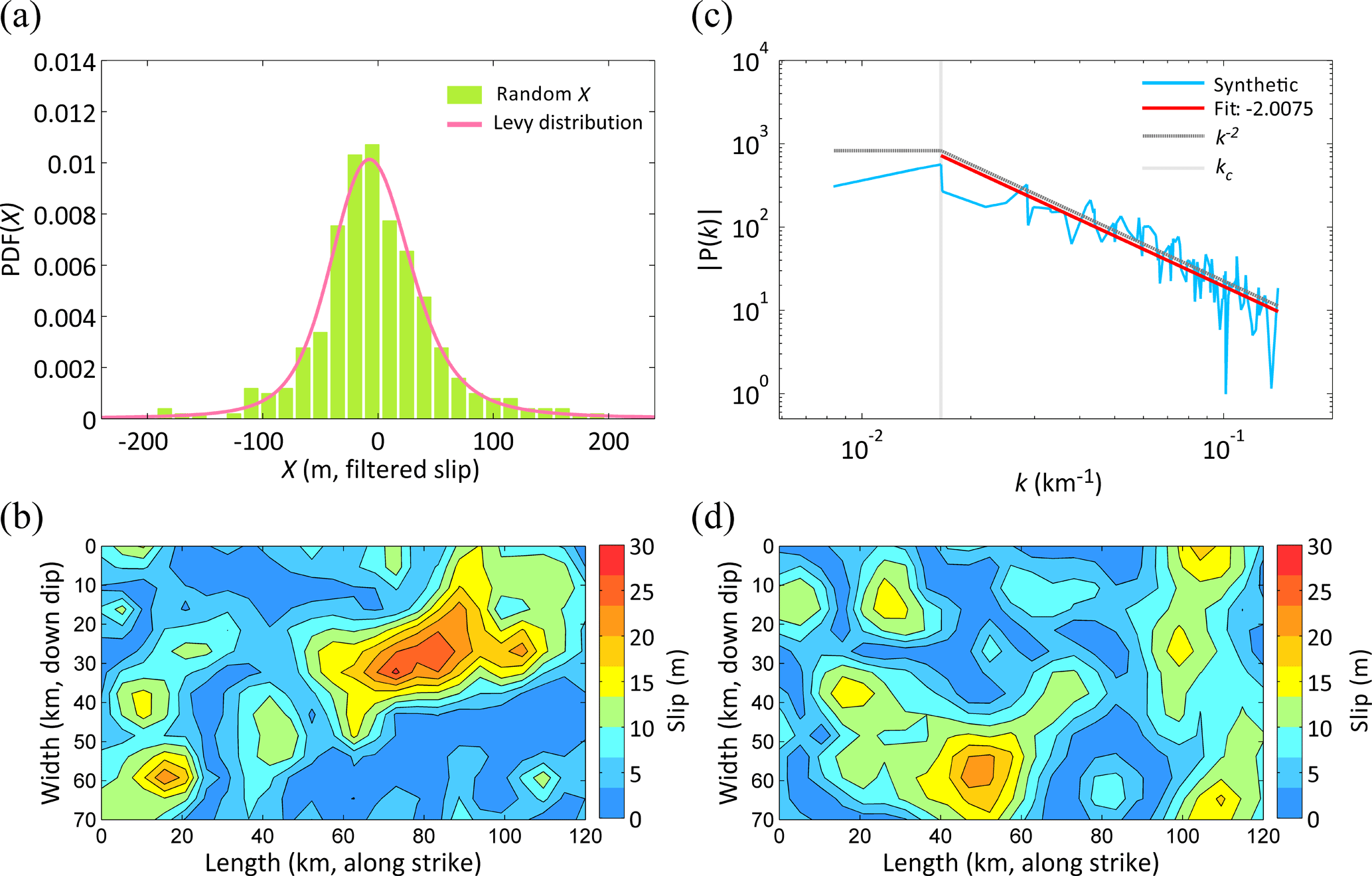
Figure 1(a) The spatially random variable is a truncated Lèvy distribution. The Lèvy parameters obtained from the Northridge earthquake were taken from Lavallée et al. (2006). (b) A stochastic slip distribution is generated by filtering the spatial random variable X in Fig. 1a. This slip pattern produces the highest maximum wave amplitude at Hualien station. (c) The slip spectrum is calculated from Fig. 1b. This slip spectrum decays with an exponent of −2 according to a characteristic corner radial wave number. This verifies that the synthetic slip distribution is identical to the k-square model and the condition of the rupture dimension. (d) This stochastic slip distribution produces the lowest maximum wave amplitude at Hualien station.

Download

The stochastic slip distribution is generated by a 2-D spatially random distribution by imposing a self-similar characteristic beyond the corner radial wave number, which is constrained by the rupture dimension, in the wave number domain. In this study, the potential rupture fault is divided into 5 × 5 km² subfaults. The grid is composed of 24×14 meshes along the strike and dip directions. The produced variable with a spatially random distribution adopts the Lèvy distribution (α=1.51, β=0.2, γ=28.3, ${\mathit{\mu }}_L=-\mathrm{0.9}$), which is the dip-slip result from Lavallée et al. (2006) shown in Fig. 1a. In Lavallée et al. (2006), the slip distribution of the Northridge earthquake was divided into the dip-slip and strike-slip directions, and they were calculated by an inverse 2-D stochastic model to obtain the values of the Lèvy PDF. The values of the Lèvy PDF, which are mentioned above, are indicative of the result of the dip-slip direction. The Northridge earthquake is a thrust earthquake (Davis, 1994), and thus, it has a faulting mechanism that is approximately similar to our scenario fault model. There are no inverted slip models of past earthquakes in the study area that can be used to conduct an analysis of the Levy PDF parameters; therefore, the Lèvy distribution in Lavallée et al. (2006) is adopted in this study. From the perspective of mathematical operations, the slip distribution in Eq. (5) represents a filtered random distribution. However, for consistency with the physical behavior over the rupture surface suggested by the results of the inverse modeling, truncation of the Lèvy distribution must be performed to constrain the extreme slip value. The synthetic slip distribution (Fig. 1b) produced by the spatially random distribution in Fig. 1a is heterogeneous, and its power spectrum obeys a k-square model at high wave numbers (Fig. 1c). The average slip of this synthetic slip distribution is 8.25 m, indicating that the earthquake energy is constant as estimated above, and the maximum slip is 31.02 m. One hundred different slip distributions are produced for the tsunami simulation representing the uncertainty in the results associated with complex rupture processes. In the 100 sets of results, the maximum slip range is between 20.17 and 37.97 m. Smooth processes are not included, nor are additional regional constraints for the slip distribution. There are two reasons for this application. The first is that we do not have information regarding where the plate interface is locked or the locations of asperities often repeat in historical events. The second is that some studies reported that the asperities extend to the boundary of the fault model (Ide et al., 2011; Lay et al., 2011; Shao et al., 2011; Yue and Lay, 2011). According to these reasons, we do not apply any additional constraints for stochastic slip distributions. Similarly, the uniform slip case constitutes a complete uniform slip distribution over the whole fault plane. Figure 1b and d demonstrate the stochastic distribution of the scenario source models causing the maximum and minimum wave heights at recording station 26 (Hualien) (Fig. 2). Both patterns affecting the propagation will be discussed in Sect. 3.1.

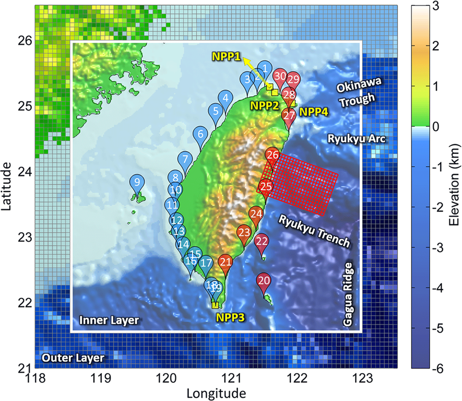
Figure 2The map of Taiwan shows the fault model and recording stations used in this study. The bathymetry is divided into two layers with different resolutions. The resolution of the outer layer is 4 min, and the resolution of the inner layer is 1 min. The red grid denotes the potential fault model (5×5 km² grid size). The pins represent 30 tidal gauges of the CWB. The red and blue colors indicate stations on the eastern and western sides of Taiwan, respectively, and the yellow squares represent the sites of nuclear power plants.

Download

2.3 Numerical tsunami simulation

Figure 2 shows the computational domain, recording stations and fault model. The potential rupture fault is divided into 5 × 5 km² subfaults, and the stochastic slip distribution model is applied to determine the amount of discrete slip on each subfault. Vertical seafloor displacements caused by slip along the rupture plane are calculated using elastic dislocation theory (Okada, 1985). The Cornell Multi-grid Coupled Tsunami model (COMCOT) is used to run the tsunami simulations. COMCOT is capable of efficiently studying the entire life span of a tsunami, including its generation, propagation, runup and inundation (Wang, 2009), and it has been widely used in studying many historical tsunami events, such as the 1960 Chilean tsunami (Liu et al., 1995), 1992 Flores Island tsunami (Liu et al., 1995), 2003 Algeria tsunami (Wang and Liu, 2005), 2004 Indian Ocean tsunami (Wang and Liu, 2006, 2007) and 2006 Pingtung tsunami, Taiwan (Wu et al., 2008; Chen et al., 2008). COMCOT solves linear or nonlinear shallow water equations for spherical or Cartesian coordinates using the finite difference method. With a flexible nested grid system, it can properly guarantee both the efficiency and the accuracy from the near-coastal region to the far-field region. Two grid layers are used to simulate the propagation of tsunamis. The Manning coefficient is 0.013 in this study, which assumes a sandy sea bottom (Wu et al., 2008). The bathymetry-adopted open data from the National Oceanic and Atmospheric Administration (NOAA) that can be download from https://maps.ngdc.noaa.gov/viewers/wcs-client/, last access: 26 March 2018 (Amante and Eakins, 2009). The resolution of the outer layer is 4 min for the solution of the linear shallow water equation, and the resolution of the inner layer is 1 min for the solution of the nonlinear form of the shallow water equation. There are 30 recording stations referring to the positions of tidal gauges maintained by the Central Weather Bureau (CWB) along the coastlines of Taiwan and the outlying islands. The CWB website presents the locations of the tide stations (http://e-service.cwb.gov.tw/HistoryDataQuery/index.jsp, last access: 26 March 2018 and https://www.cwb.gov.tw/V7e/climate/marine_stat/tide.htm, last access: 26 March 2018). These locations are shifted slightly to the grid nodes to accurately record the data. Table 1 presents the locations and water depths of the recording stations in the computational mesh.

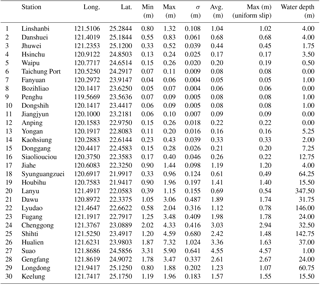
Table 1The maximum, minimum and average wave heights with their standard deviations for the PTA probability distributions (in meters) with the maximum wave heights from the uniform slip model. The water depths at the stations in the computational mesh are also included.

Download Print Version | Download XLSX

3.1 Initial water elevation and energy propagation

The static vertical displacement of the ocean floor is modeled using elastic dislocation theory (Okada, 1985) with a static slip distribution. The vertical seafloor displacement is modeled as the initial water level, and the horizontal component of the seabed displacement is not included in the simulation. Figure 3a shows the initial water elevations produced by a uniform slip distribution, and Fig. 3b exhibits the maximum free-surface elevation during the propagation. Figure 3c and e demonstrate the initial water elevations produced by the stochastic slip distributions (Fig. 1b and d). The initial water elevation with a uniform slip distribution is simple and smooth, but those with stochastic slip models are more complex and relatively heterogeneous. Nonuniform slip causes an apparent change in the wavelength distribution of the initial free-surface elevation (i.e., the potential energy distribution), which affects the path of energy propagation. In the uniform slip scenario, the maximum free-surface elevation pattern is straightforward and clearly controlled by the topography. However, many strong and seemingly chaotic paths of wave energy appear in the nonuniform slip scenarios, and the free-surface field exhibits additional uncertainties in terms of the flow. In Fig. 3b, the maximum free-surface elevation mainly propagates toward two places where the seafloor bathymetry becomes shallow relative to the deep areas northeast of Taiwan, as shown in Fig. 2. Although the propagation paths due to the nonuniform slip distributions (Fig. 3d and f) also have the same characteristics, it is notable that the paths followed by the wave energy differ depending on the rupture pattern. To the northeast of Taiwan in Fig. 3f, there is a strong wave path connecting the two higher-elevation areas of bathymetry. However, this behavior is not observed in Fig. 3b and d. In addition, the maximum elevation on the footwall in Fig. 3d is higher than that in Fig. 3f. In Fig. 3b, the high elevation appears only along the coast on the footwall side. These results indicate that the wave energy variation depends on the rupture pattern, thereby causing differences in the wave paths and leading to completely different tsunami amplitudes.

Figure 3Panels (a), (c) and (e) are the initial water elevations, and the color bars represent the elevation of the initial water surface. Panels (b), (d) and (f) are the maximum free-surface elevation (i.e., the distribution of the energy path), and the color bars represent the elevation of the maximum free-surface. Panels (a) and (b) display the results with a uniform slip distribution. Panels (c) and (d) display the results from Fig. 1b. Panels (e) and (f) display the results from Fig. 1d. The seafloor elevation fundamentally dominates the tsunami propagation, but the slip distribution also has a strong influence. In (a, c and e), yellow squares represent NPPs; in (b, d and f), the NPPs are represented by open squares.

Download

3.2 Wave characteristics

Thirty stations located along the coastlines are available for recording the amplitude of the tsunami wave height. Relative to the other stations, stations 25 (Shihti), 26 (Hualien) and 27 (Suao) are situated near the potential rupture fault, and they have high wave amplitudes and enormous variations in the tsunami simulations of 100 different slip distributions; consequently, the time series of the wave heights at these stations are shown as an example (Fig. 4). The time series of the wave heights at the other stations are shown in the Supplement. The variability in the distribution of the initial free-surface elevation results in substantial phase changes and different wave heights. It is worth noting that the average of the disordered and chaotic time series produced by the 100 different slip distributions is almost identical to the results of the time series produced by the uniform case. This implies that the uniform slip distribution simply represents an average result and that it cannot represent all of the possible situations.

According to the statistical results from 100 different slip patterns (Table 1) for 30 stations, Hualien station has a maximum wave amplitude of 7.32 m, and its maximum wave amplitude interval ranges from 1.87 to 7.32 m, which constitutes the widest interval for any recording site, and the standard deviation of this distribution is 1.024 m. These findings indicate that Hualien station has a high uncertainty in this scenario. However, the maximum wave amplitudes from the uniform slip distribution are relatively lower than those from the stochastic results. Following the above findings, we need to consider whether the estimations from the uniform slip case are appropriate for hazard analysis by focusing on the maximum wave amplitude issue.

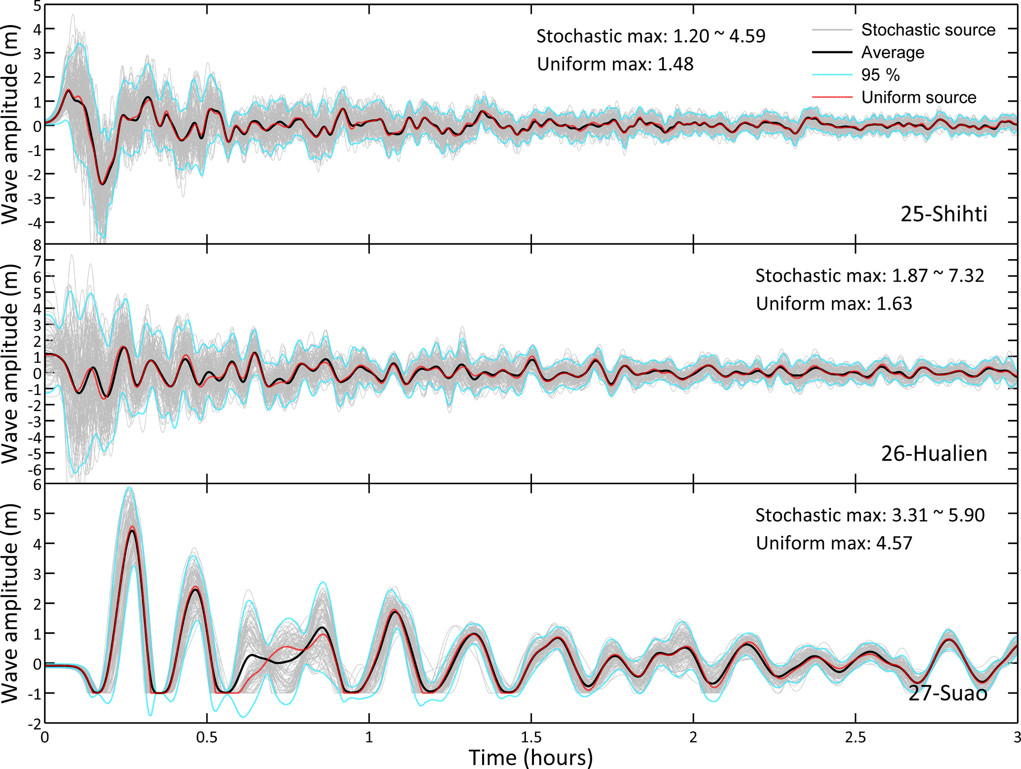
Figure 4The time series of the wave heights recorded at stations 25 (Shihti), 26 (Hualien) and 27 (Suao). Gray lines represent the time series of 100 different slip distributions, black lines represent the averages of the gray lines, blue lines represent the 95 % confidence intervals, and red lines are the time series produced using uniform slip distribution. Parts of the wave heights at station 27 are lower than the water depths, and thus, these curves have been truncated.

Download

3.3 The peak tsunami amplitude probability

According to the results of our simulations, we calculate the probability of the peak tsunami amplitude (PTA) at each recording station as shown in the histogram of Fig. 5. To verify the representativeness of the PTA probability distributions, another 100 sets of different slip distributions are produced and simulated under the same seismic conditions. In Fig. 5, the shapes of the PTA distributions from another 100 sets (black lines) are similar to the shapes of the histograms from the first 100 sets. These results verify the representativeness of the PTA probability distributions produced from 100 sets of slip distributions. This test also reinforces the reproducibility of our simulations and demonstrates that the number of simulations is roughly satisfactory for statistical analysis. Of course, the more slip distributions we use, the more comprehensive and stable the range we obtain.

Figure 5The probabilities of the PTA along the coast of Taiwan (blue: stations 1 ∼ 19, red: stations 20 ∼ 30). The histograms display the PTAs derived from 100 different slip simulations. The black lines represent the results from another 100 simulations, and the orange lines represent the PTA obtained using a uniform slip distribution. The PTA probability distribution gives a clear PTA range and its occurring probability. The map of Taiwan shows the station locations and the sites of four NPPs (yellow squares).

Download

In Fig. 5, the PTA distributions for the stations in eastern Taiwan (red markers) have much higher values than those in western Taiwan (blue markers) due to the specified location of the tsunami source. The shapes of the PTA distributions in eastern Taiwan resemble lognormal distributions, while those in western Taiwan resemble normal distributions. We suppose that the attenuation of the wave propagation causes the lognormal distributions to degenerate into normal distributions. The PTAs produced by a uniform slip distribution are generally located in the middle of the PTA distributions. Both PTA values (i.e., the value of the PTA from the uniform slip distribution and those from the stochastic slip distribution models) decrease with distance from the potential fault due to the attenuation of the wave propagation (Fig. 5 shows the results for all stations, and Fig. 6 shows the results for stations 20 through 30 in eastern Taiwan). However, some stations, e.g., stations 17, 19 and 21, do not precisely follow this trend; this could be the result of the coastal topography and the presence of an energy channel. From Fig. 3d, in comparison with the adjacent coastline, station 21 is located exactly where the wave energy gathers. In addition, broad distributions are frequently observed at promontories along the coastline and are caused by complex propagation path effects between the source region and the recording locations (Geist, 2002). There are many compound factors that affect the tsunami propagation and maximum wave height. Figure 6 presents the relation between the distance and wave height and shows the PTA distributions following Fig. 5. The x axis presents the shortest distance between the stations and fault plane. On the footwall side, stations 20 and 22, which do not directly face the energy propagation path (Fig. 3f), are located on islands off the coast of Taiwan; consequently, their PTA distributions are lower than those of stations 21 and 23, even though the distances from the potential fault are similar. On the hanging wall, station 29 is farther from the coastline of Taiwan than other stations; however, because of the real location of the station and its numerical grid setting, its PTA distribution is lower than that of station 30 (Fig. 3b). The ranges of the PTA distributions converge with increasing distance on both sides of the fault. Moreover, the PTA distributions and their average values roughly exhibit a linear decrease with increasing distance except for stations 25 and 26. In contrast, these two stations in the near field are directly affected by initial water elevation, and thus, the PTAs caused by uniform slip are quite low.

Although the seismic parameters have already been defined as constants in our experiment, there exists an uncertainty in the PTA, which is not a constant value. Hence, the uniform case cannot provide this uncertainty, and thus, the PTA could be underestimated. The results give specific PTA ranges, which represent the wave height uncertainties for the scenario of earthquakes originating from the Ryukyu Trench. It is therefore necessary to consider the effects of a heterogeneous slip distribution to comprehensively assess the tsunami hazard.

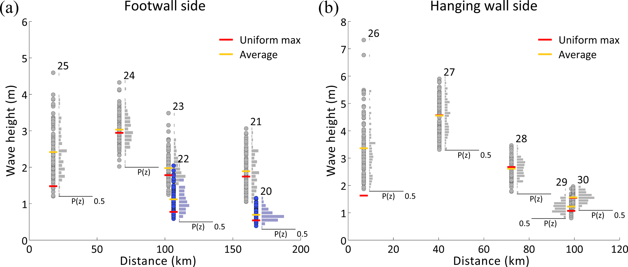
Figure 6The relation between the distance and wave height for stations 20 to 30 in eastern Taiwan. Panel (a) is the station on the footwall side. Stations 20 and 22 (blue color) are off the shoreline of Taiwan. Panel (b) represents the stations on the hanging wall side. Both sides roughly exhibit a linear decay and range of uncertainty converging with increasing distance for the tsunami amplitude. Red bars show the PTA of the uniform slip distribution, and yellow bars show the average of the PTAs from the stochastic slip models.

Download

4.1 Tsunami

Most coastlines threatened by near-field tsunamis, such as the coasts of Chile, Japan and Indonesia, are parallel to the trench axis of the associated subduction zones. Many tsunami events, including the M_w 8.8 Chile earthquake in 2010 (Lay et al., 2010; Fritz et al., 2011), the M_w 9.0 Tohoku earthquake in 2011 (Goda et al., 2015; Goda and Song, 2016), the M_w 9.1 Sumatra earthquake in 2004 (Lay et al., 2005), and the M_w 8.1 Mentawai earthquake in 2010 (Satake et al., 2013), have occurred along these regions. However, the potential rupture fault in this study along the southernmost Ryukyu subduction zone is perpendicular to the coast of Taiwan, which directly affects the first wave motion. The first motion on the footwall is up; conversely the first motion on the hanging wall is down. As a result, the coastline retreats from the land to the sea as the first tsunami wave approaches, allowing people additional time to leave the seafront.

The effect of a heterogeneous slip distribution is important and necessary for near-field estimations (Geist, 2002 and Ruiz et al., 2015). Figure 5 shows that the PTA distributions in the near field are broad, and they narrow with increasing distance from the potential fault. The uncertainty in the near field is higher than in the far field. At most of the eastern stations, the values of the average PTA approach uniform results, but the uniform slip results at stations 25 and 26 are close to the minimum PTA (Table 1). Geist (2002) presented the average and extreme nearshore PTA calculated for 100 different slip distributions and compared them with the uniform slip results (Fig. 6a in Geist, 2002). The range of the PTA also becomes narrower with increasing distance. The values from the uniform slip distribution and the average PTA are similar, but some of the average values are close to the minimum PTA between approximately 19 and 19.5^∘ N. Similar characteristics of the average PTA and the results from the uniform case are observed in different regions. The average PTA is equal to the uniform slip result in the nearshore region, but this could be caused by other factors (e.g., distance to the tsunami source, propagation path, initial water elevation) that shift the average PTA toward the minimum PTA.

Four nuclear power plants (NPPs) are located on the island of Taiwan. According to the numerical results, we infer that the mean PTA in the coastal area of NPP4 ranges from approximately 2 to 3 m. The distribution at this plant may be wider than those at other nuclear power plants due to its position relative to the tsunami source. Moreover, NPP4 is located on the shore of a bay with a curved shape; the magnification effect from the geometrical shape of the bay may serve to enhance the PTA therein. NPP3 also exhibits this condition insomuch that the energy is concentrated at the location of the plant (Fig. 3b, d and f). For the coastal areas around NPP1 and NPP2, the PTA distributions are between 1 and 2 m. The coastlines of these two nuclear power plants slightly face the direction of tsunami propagation, and thus, their PTAs should be higher than those along adjacent coastlines (Fig. 3b, d and f). In general, under this scenario, the coastline at NPP4 has the largest threat. Although NPP3 is far from the tsunami source, it faces a wave height of approximately 1.5 m on average with a ±0.5 m range of uncertainty. However, NPP3 is closer to the Manila subduction zone, and thus, it could be threatened by a tsunami originating from the Manila Trench. In contrast, the coastlines of NPP1 and NPP2 are relatively safe and have fewer uncertainties with regard to the PTA.

The use of heterogeneous slip patterns clearly delineates the range of possible waveforms and provides more information on latent uncertainties in the wave height. The 95 % confidence intervals for the wave height from 100 sets in each time series provide us with a specific range for the amplitude of the tsunami wave (Fig. 4). According to these time series, we are aware of the periods of tsunami runup and runoff and can prepare supporting policies to reduce associated disasters. For example, a nuclear power plant uses a trench from the ocean to intake water to cool the reactor; thus, if the sea level is too low to take in water, the temperature of the reactor will rise excessively, causing a nuclear disaster. Based on the results of simulations, we can estimate how much water should be stored for tsunami runoff. This issue requires more attention in Taiwan because four nuclear power plants are located near the coast.

4.2 Stochastic slip model

The results of the tsunami simulations illustrate that the effect of the slip distribution on the rupture plane has significant effects on the wave propagation and wave height. The correctness of this slip distribution determines whether the wave height calculations represent a useful reference. However, some parameters of the stochastic models could influence the synthetic slip distributions. For instance, the exponent of the slip spectrum is associated with the roughness of the slip distribution. Higher exponential values inhibit the powers of high wave numbers, leading to smoother slip distributions; conversely, lower values lead to rougher slip distributions. In general, the k-square model needs to be followed. Furthermore, the interpolation of the slip distribution for a given geometry will affect the exponent of k (Tsai, 1997). Interpolation will smooth the original pattern. The powers of short wave numbers will be depressed and the powers of long wave numbers will be enhanced. Moreover, the random spatial variability of the slip distribution is relatively critical. According to Lavallée and Archuleta (2003) and Lavallée et al. (2006), we adopt the truncated non-Gaussian distribution for the spatial variability. This truncation limits the non-Gaussian distribution to a particular range. However, extreme truncation will cause the heavy-tailed characteristic of this distribution to become less pronounced or even disappear, similarly to a Gaussian distribution. In mathematics, the synthetic slip distribution is a filtering process insomuch that the characteristics of a heavy-tailed distribution affect the extrema of the slip distribution. The maximum slip will be greater as the truncated range increases, and the maximum slip may exceed reasonable values if the truncated range is excessively wide. Therefore, the parameters must be chosen carefully to match the observations acquired by inversion.