Estimating network related risks: A methodology and an application in the transport sector

Hackl, Jürgen; Lam, Juan Carlos; Heitzler, Magnus; Adey, Bryan T.; Hurni, Lorenz

doi:https://doi.org/10.5194/nhess-18-2273-2018

Articles | Volume 18, issue 8

https://doi.org/10.5194/nhess-18-2273-2018

Articles | Volume 18, issue 8

Research article

27 Aug 2018

Research article |

| 27 Aug 2018

Estimating network related risks: A methodology and an application in the transport sector

Jürgen Hackl, Juan Carlos Lam, Magnus Heitzler, Bryan T. Adey, and Lorenz Hurni

Abstract

Networks such as transportation, water, and power are critical lifelines for society. Managers plan and execute interventions to guarantee the operational state of their networks under various circumstances, including after the occurrence of (natural) hazard events. Creating an intervention program demands knowing the probable direct and indirect consequences (i.e., risk) of the various hazard events that could occur in order to be able to mitigate their effects. This paper introduces a methodology to support network managers in the quantification of the risk related to their networks. The methodology is centered on the integration of the spatial and temporal attributes of the events that need to be modeled to estimate the risk. Furthermore, the methodology supports the inclusion of the uncertainty of these events and the propagation of these uncertainties throughout the risk modeling. The methodology is implemented through a modular simulation engine that supports the updating and swapping of models according to the needs of network managers. This work demonstrates the usefulness of the methodology and simulation engine through an application to estimate the potential impact of floods and mudflows on a road network located in Switzerland. The application includes the modeling of (i) multiple time-varying hazard events; (ii) their physical and functional effects on network objects (i.e., bridges and road sections); (iii) the functional interrelationships of the affected objects; (iv) the resulting probable consequences in terms of expected costs of restoration, cost of traffic changes, and duration of network disruption; and (v) the restoration of the network.

Download & links

Article (PDF, 4114 KB)

Supplement (3986 KB)

Download & links

Article (4114 KB)
Supplement (3986 KB)
BibTeX
EndNote

How to cite

How to cite.

Dates

Received: 19 Dec 2017 – Discussion started: 02 Jan 2018 – Revised: 16 Jul 2018 – Accepted: 31 Jul 2018 – Published: 27 Aug 2018

1 Introduction

Managers of networks, such as transportation, water and power, have the continuous task to plan and execute interventions to guarantee the operational state of their networks. This also applies in the aftermath of (natural) hazard events. As the resources available to managers to protect their networks are limited, it is essential for managers to be aware of the probable consequences (i.e., risk) in order to set priorities and be resource-efficient (Eidsvig et al., 2017). Consequences are often expressed in monetary values, and these are distinguished between direct costs (e.g., costs related to clean up, repairs, rehabilitation and reconstruction) and indirect costs (e.g., in the transport sector, costs related to additional travel time, vehicle operation and an increase in the number of accidents). Indirect costs have a wide spatial and temporal scale (Merz et al., 2010) and are potentially larger than direct costs (Vespignani, 2010).

Conducting a risk assessment can help identify probable hazard events, and evaluate their impact on networks and users. Nonetheless, conducting such assessments can be a particularly challenging task due to the large number of scenarios (i.e., chains of interrelated events) that need to be taken into account, the modeling of these events, the relationships among them, and the availability of support tools to run the models in an integrated way. In building scenarios, multiple types of hazards need to be considered, along with the complex nature of networks, specifically their large number of objects, their spatial distribution, and functional interrelationships. Moreover, it is important to estimate the performance of networks during the hazard events and through the recovery to an adequate level of service that is driven by restoration strategies (Lam and Adey, 2016). Therefore, network managers need to think of ways to model the cascade of events, interdependencies, and the propagation of uncertainties (Hackl et al., 2015).

As a result of these challenges, risk assessment methods for networks have been the subject of increasing research interest in recent years. Most research has been focused either on the technical aspects of hazards or those of networks. In the first case, scholars have focused on improving the understanding, the modeling or the prediction of single hazard events (Apel et al., 2004; Pritchard et al., 2015; Schlögl and Laaha, 2016; Pellicani et al., 2017) without explicitly considering the complexity and dynamics of networks. In the second case, scholars have investigated the vulnerability¹ (Jenelius et al., 2006; Rupi et al., 2015; Shabou et al., 2017) or resilience (He and Liu, 2012; Bocchini and Frangopol, 2012; Vugrin et al., 2014) of networks due to disruptions, without evaluating the cause and/or the probability of such disruptions.

Some work has been conducted to consider multiple hazards and their effects (i.e., multiple vulnerabilities and consequences) in a unified framework (Komendantova et al., 2014; Mignan et al., 2014; Gallina et al., 2016). Assessing the risk in such a way is relatively new, and until now only partially developed by experts with different backgrounds such as statistics, engineering and various fields of geosciences (Komendantova et al., 2014). Only a limited number of scenario-based and/or site-specific studies have been proposed due to the difficulty and novelty of the task (Mignan et al., 2014). Having a diverse team of experts, whose discipline-specific approaches to risk assessment may differ, presents an additional challenge: their contributions are not always easy to aggregate to a level that is useful for network managers. In addition, current research also shows the need to take into account the spatial-temporal quantification of risks across different levels of scale for future sustainable risk management (Fuchs and Keiler, 2008; Fuchs et al., 2013).

Open research. In conclusion, there has been little work to bring research outputs concerning the modeling of hazard events and network vulnerability together in a way that their spatial and temporal uncertain behaviors are assessed in a unified framework that fosters multidisciplinary collaboration.

Contributions. To overcome these challenges, this article presents the application of a novel risk assessment methodology. The methodology can be used to investigate multiple scenarios, starting from the modeling of a source event (e.g., rainfall, fault rupture), and ending in the estimation of the probable consequences of related societal events (e.g., communities without access to transportation, water or power service). While the methodology is applicable to different types of hazards, networks, regions, sizes of regions, and levels of resolution, the application of the methodology is illustrated on a regional road network in Switzerland prone to floods and mudflows. Specifically, this work advances the state-of-the-art in the field of network related risks due to hazard events as follows.

The risk of a complete chain of events, from a source event to its societal events is quantified over space and time. In the application, this means considering precipitation, runoff, flood, mudflows, (physical) damages, functional losses, traffic flow changes, and restoration interventions. The presented links between cascading hydrometeorological hazards, a road network and society will be of interest to the international research community and practitioners working in the fields of network management, urban planning, public policy, and emergency response.
When quantified, risk can be categorized into probable direct and indirect costs, with the latter estimated throughout the hazard events and restoration periods, not just immediately after the occurrence of the hazard events. In the application, direct and indirect costs included costs of interventions, prolongation of travel time, and missed trips, allowing for the evaluation and comparison of the socio-economic impacts of the multiple hazard scenarios considered.
The simulation-based approach supports the inclusion of uncertainties and their propagation throughout the risk model. The application includes results related to the simulation of 1200 rainfall events, causing floods of return periods ranging from 2 to 10 000 and, depending on the rainfall intensity and duration, stochastically triggering a number of mudflows in the area. Furthermore, as suggested by Lam et al. (2018 a), the approach can support the testing of additional scenarios based on uncertain relationships (e.g., fragility functions relating hazard intensities with damage state exceedance probabilities).
A novel simulation engine was constructed as the computational platform to estimate risk, supporting the combination of models from different disciplines, and their modular update and replacement. The application demonstrates the coupling of existing models and information from literature in geosciences, engineering, network theory, transportation, and economics.

The example application makes further research contributions on ways that road network managers can estimated the risk related to their networks due climate-related hazard events. With a changing climate, exacerbated by an increase in urbanization, the frequency of extreme hydrometeorological hazard events is expected to rise, impacting economic corridors, disrupting supply chain, and stressing emergency and rescue operations, among other effects (Keiler et al., 2010; Fuchs et al., 2017). As a result, special focus is now given to these hazard events and their associated risks. In times of scarce public resources and increasing incidences and damages caused by floods (Bowering et al., 2014), network managers have the need to become increasingly aware of their causes and consequences so that they can appropriately manage their risks, for example, through the adaptation of networks (Elsawah et al., 2014) or the planning of actions following a hazard event (Taubenböck et al., 2013). A number of methods have been developed to quantify the damages and costs due to floods (Merz et al., 2010; Hammond et al., 2015). Nevertheless, most of these studies have been focused on buildings and the estimation of direct costs.

In the transport sector, some work has been done to consider the probable direct costs of floods (e.g., Scawthorn et al., 2006; Deckers et al., 2009; Bowering et al., 2014), but these works have often neglected the spatial and temporal attributes of these networks. Only a few scholars have investigated flood risk in combination with the actual changes in traffic flow. Dawson et al. (2011) implemented an agent-based model to simulate the human response to floods considering different storm surge conditions. Suarez et al. (2005) studied the impacts of floods and climate change on the urban transport system of the Boston Metro Area, using a conventional analytical framework for simulating traffic flows under different flood scenarios, changes in land use, and demographic and climatic conditions. In both cases, the direct costs resulting from damages were not taken into account. Furthermore, only the events unfolding during the hazard events period were analyzed, and hence, no network restoration was considered, which is essential for quantifying indirect costs.

While floods are the most common rainfall-triggered hazard events in mountainous areas, landslides, including mudflows, are second in place. As road networks in these areas generally have a low level of connectivity (e.g., remote villages that are only connected by few mountain roads), there is a high probability that connections between some areas within a road network can be interrupted when one or a limited number of objects fail (Rupi et al., 2015). Usually, risk estimates related to networks, including road networks, due to landslides have been obtained by overlapping hazard and consequence maps (Ferlisi et al., 2012; Pellicani et al., 2017) and thus the indirect costs for specific hazard scenarios have not been considered.

In general, according to Mattsson and Jenelius (2015), there are two dominant types of risk assessment methods for transport networks. The first set of methods is rooted in graph theory, and is focused on the study of the topological properties of the networks. This analytical approach requires network topology data and considers the importance of different edges (Jenelius et al., 2006; Rupi et al., 2015), cascading failures (Dueñas-Osorio and Vemuru, 2009; Hackl and Adey, 2017), and interdependencies between different networks (Thacker et al., 2017). The second group of methods is focused on understanding the dynamic behavior exhibited on networks (e.g., traffic flow) through the use of transportation system models. While this approach has the potential to provide a more complete description of society-related consequences than graph-theory-based methods, the approach often requires extensive data and significant computational resources, limiting the modeling of this dynamic behavior to only a few deterministic scenarios.

This work is organized as follows. A brief overview of the risk assessment methodology is presented next in Sect. 2. Section 3 contains a description of the main features of the application to illustrate the use of the methodology. The results obtained from the application are presented in Sect. 4 while a discussion about the findings, and the advantages and shortcomings of the methodology and the models used are given in Sect. 5. Concluding remarks and suggestions for future work are given in Sect. 6.

2 Risk assessment methodology

The purpose of the risk assessment methodology is to support network managers in the quantification and subsequent management of risk. The methodology is founded on the principles of systems engineering (Adey et al., 2016) and thus the methodology is structured keeping in mind that (i) different decisions require different models, (ii) models provide different levels of detail, and (iii) this is an iterative process, requiring changes as data and model insufficiencies are discovered, and new data and models become available. Considering these principles, the risk assessment methodology is structured as follows:

Set up risk assessment – the rough outline of the planned risk assessment.
Determine approach – the agreements on how to perform the risk assessment, including the involved parties and the activities to conduct.
Define system representation – the agreements on system behavior, system boundaries, assumptions and limitations.
- Define boundaries – the parts of the system to be analyzed, both spatially and temporally.
- Define events – the events to be analyzed.
- Define relationships – the relationships between events.
- Define scenarios – the scenarios combining the events and relationships.
- Determine tools – the selection of tools, models and software to analyze the scenarios.
Estimate risk – the computed probabilities of the scenarios and their consequences.
Evaluate risk – the interpretation of the risk estimates.
Update approach and/or system representation – the parts of the system to be analyzed in more detail in order to decrease the uncertainties of the result.

The considered events are described using generic categories: source, hazard, object, network and societal. Source events are ones that, at least from a modeling perspective, are considered to simply happen with a certain probability, and may lead to hazard events. Each object in the network is vulnerable to these hazard events, which may cause damage and/or functional losses. These impacts can be the origin of failures in the network resulting in a deficient level of service. These effects can impair the functioning of society during the hazard events and restoration periods. The execution of restoration interventions enables the network to provide an adequate level of service again by changing the state of damaged objects.

Such a chain of events can be assembled using a novel simulation engine (Heitzler et al., 2018) that supports the coupling of multiple heterogeneous models, where a given model encapsulates the behavior and state of a part of the system. To support the data exchange between models, models are grouped into modules, with each module comprising distinct execution instructions and data requirements. The data consist of model parameters, static input (e.g., the location of mudflows, the extent of the road network, the distribution of a variable to sample from) and the states of models in other modules (e.g., to determine the damaged objects, the water extend from a flood model is needed). The advantage of such a modular approach is that only input and output have to be defined for each module. Consequently, different models and software solutions can be used to simulate scenarios. For example, a flood can be simulated using a custom model or off-the-shelf software such as HEC-RAS (Brunner, 2016), Basement (Vetsch et al., 2018), etc., without having to modify other models. This approach allows scientists to implement and test their own models, including their effects on risk estimations.

Once the modules and module interfaces are defined (as a reference, see Fig. 1 for a schematic representation of the modules used in the application), the network manager can conduct the risk assessment. Risk is here expressed in terms of expected monetized consequences, calculated as a product of the probability of occurrence of a certain scenario and the associated costs of that scenario – both the direct (dc) and the indirect costs (ic) should be considered. Their cost functions C^dc and C^ic are associated with the modeled societal events E^soc that occur as a result of object events E^obj and network events E^net, and that can be traced back to hazard events E^haz and source events E^src. This representation (for a given source event, see Eq. 1) can also be used when considering multiple hazard events. As the spatial and temporal correlation between events is considered, risk can be said to be spatially and temporally distributed (i.e., risk estimates vary in space within a defined area of study, and in time within a defined period of analysis).

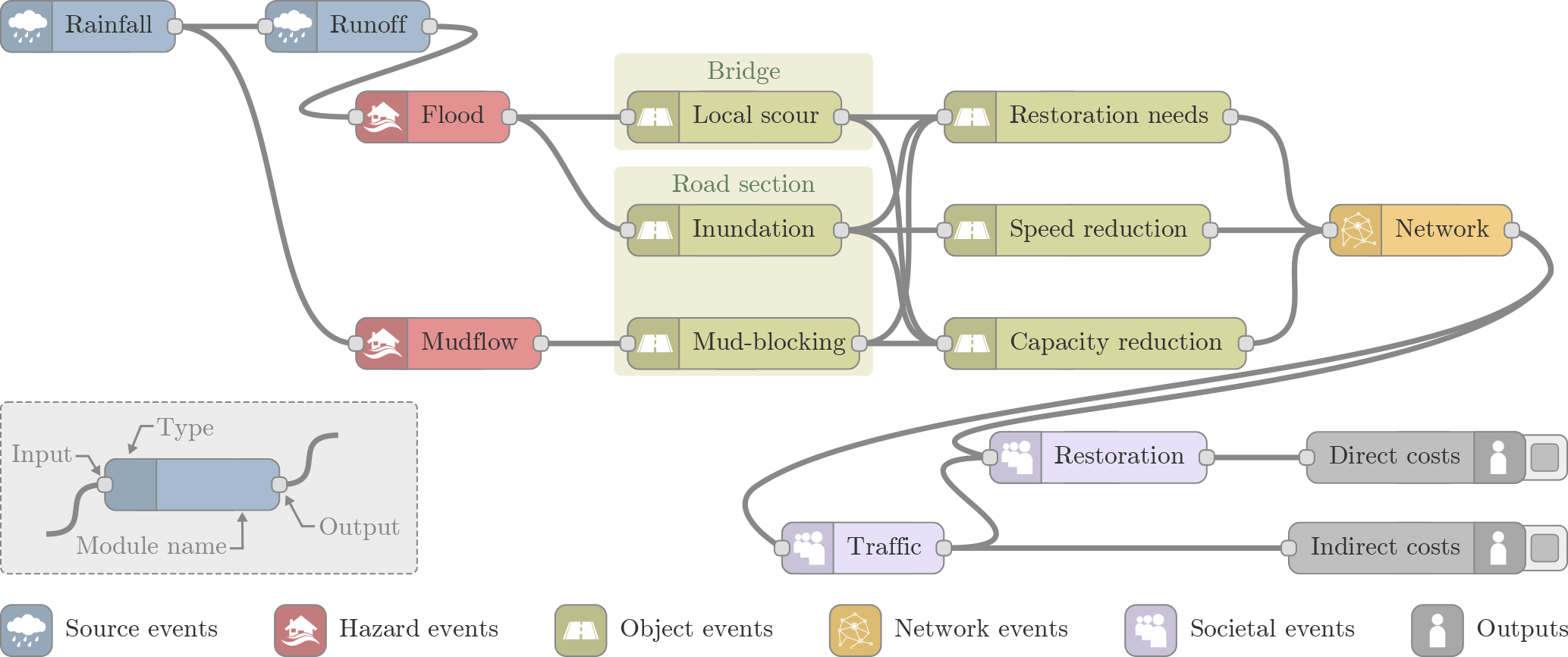
https://www.nat-hazards-earth-syst-sci.net/18/2273/2018/nhess-18-2273-2018-f01

Figure 1Schematic overview of the modules used for the application. Modules, represented by nodes with certain inputs and outputs, are related to the events that need to be modeled to estimate risk. The assessment starts with the modeling of a random rainfall and its corresponding runoff. Estimated discharge values at river stations of interest are used to simulate the flood propagation, including the inundation of the area. A mudflow can be randomly triggered during the rainfall if accumulated precipitation values exceed certain thresholds. In the next step, expected damages (i.e., bridge local scour, road section inundation, road section mud-blocking), functional losses (i.e., speed reduction, capacity reduction), and restoration needs (i.e., restoration cost, restoration time) are determined for each affected object in the network. The updated states of individual objects help define the new state of the entire network. The traffic through the network is then simulated. Restoration interventions are executed to enable the network to provide an adequate level of service again by changing the state of damaged objects. The costs for the restoration are accounted as direct costs, while the costs related to additional vehicle travel time through the network and missed trips are accounted as indirect costs.

Download

\begin{array}{l} R | E^{src} = \overset{probability}{\overset{︷}{P [E^{haz} | E^{src}]}} \\ (1) & \cdot \overset{consequences}{\overset{︷}{(\underset{direct}{\underset{︸}{C^{dc} (E^{soc} | E^{obj}, E^{haz})}} + \underset{indirect}{\underset{︸}{C^{ic} (E^{soc} | E^{net}, E^{obj}, E^{haz})}})}} \end{array}

Furthermore, network managers may be often interested in investigating the effect of hazard loads on their critical objects. Therefore, managers need to be given the option to select hazard events based on the periodicity of the manifested site-specific hazard loads (i.e., managers may not be as concerned with selecting a hazard event based on the return period of the preceding source event). Then Eq. (1) can be modified by first selecting the hazard events according to the return periods related to the site-specific loads (i.e., risk is conditioned on the hazard event (ℛ|E^haz) and thus the probability of occurrence of a scenario is defined as ℙ[E^src|E^haz]). For example, the network manager might be interested to evaluate a flood with a return period of 100 years in a specific point in the network. In this case, the simulation engine finds a suitable rainfall that causes the flood of interest.

3 Application

The application presented in this section is used to demonstrate the usefulness of the methodology considering a specific problem. The application shows the design and implementation of an assessment focused on estimating the risk related to a road network in the Canton of Grisons in Switzerland. In the study, the network was exposed to rainfall, which caused multiple hazards, specifically riverine floods and mudflows. At the same time, these events led to direct costs linked to clean-up, repair, rehabilitation and reconstruction activities, and indirect costs associated with loss of connectivity and temporal prolongation of network user travel time, linking the modeling of these latter effects with the dynamics of the network. A large number of uncertain rainfall leading to floods of multiple return periods was considered in the analysis.

The data used for this application were representative of actual entities and processes in the region, or were derived from such data. Moreover, the models selected for the application were chosen considering the need to keep the computational time low. The authors of this paper are fully aware that other models may be available in the literature, some of which are more sophisticated and precise, and hence, demand much more detailed data than the data that were available. Nonetheless, the selection of data and models was sufficient for illustrating the use of the methodology. The proposed risk assessment methodology is unaffected by these limitations, and the modular simulation engine supports the updating of data and models.

3.1 Area of study

The investigated road network is located in the Rhine Valley between Trin and Trimmis (Fig. 2). This target area is located around the city of Chur, the capital of Grisons, the largest and easternmost canton of Switzerland. It is the largest city in Grisons with approximately 34 500 inhabitants and a large business center. Chur is also an important transportation hub, linking Switzerland, Germany, Austria, and Italy. The Canton of Grisons is crossed in a north–south direction by the A13 motorway² The considered road network comprises ca. 121 bridges and 605 km of roads, including 51 km of national roads.

https://www.nat-hazards-earth-syst-sci.net/18/2273/2018/nhess-18-2273-2018-f02

Figure 2The area of study is located in the east of Switzerland. The red areas indicate the considered catchments of the Rhine rivers. The risk assessment was performed on the road network located within the green boundary. The data to calibrate and validate the rainfall, runoff, and flood model were collected from nine precipitation measurement stations (green nodes) and seven gauging stations (red nodes). Historical landslides, floods, and their damages to road networks are illustrated as symbols, where their size represents the magnitude of the associated direct costs. Four hazard events with damages over CHF 5 million occurred within the last decade in the investigated area (Felsberg, Chur, and Trimmis).

Download

Lake Toma in Grisons is generally regarded as the source of the Rhine. Its outflow is called Rein da Tuma, and after a few kilometers, the outflow forms the Anterior Rhine. The Anterior Rhine is about 76 km and has a catchment area of 1512 km². The Posterior Rhine is the second tributary of the Rhine, with less length, but a larger discharge than that of the Anterior Rhine. The basin of the Posterior Rhine is approximately 1698 km². The river begins to be called the Rhine at the confluence of the Anterior Rhine and Posterior Rhine in Reichenau. For both rivers, detailed runoff and flood information are available from the stream gauging stations in Ilanz (No. 2033, 2498) and Fürstenau (No. 2387). Both towns are at the considered boundaries of the investigated area. Another stream gauging station is located in the study area at Domat/Ems (No. 2602), which was used as a reference point for the hydraulic model. Nine precipitation gauging stations with sufficient historical series are available in the basins under consideration. Precipitation data since 1887 are available to determine and calibrate extreme rainfall.

The investigated area is exposed to floods and landslides on an annual basis as the historical records of the Swiss Flood and Landslide Damage Database³ show. Figure 2 illustrates some of the recorded hazard events (45 in the area of interest) from 1975 to 2013 that affected networks⁴. From these, 27 events fell into the category of floods/debris flow, 13 events fell into the category of landslides (other than debris flow), and the remaining 5 events were classified as rockfalls. The costs were in the range between CHF 10 000 and CHF 6.85 million. According to the dataset, four events caused “high/catastrophic” damages while five and 36 caused “medium” and “minor” damages, respectively⁵. Consequences included 12, 31 and two disruptions on the railway network, the road network and traffic, and the power supply, respectively. Over the period of 38 years, two bridges were severely damaged and three bridges collapsed. One of the worst floods in recent history occurred in 2005. This flood was responsible for approximately CHF 695 million in damages to roads and railways in Switzerland (Bezzola and Hegg, 2007).

3.2 Application of the methodology

The setup of the risk assessment described in the opening of Sect. 3 was complemented by additional specifications. The assessment only considered rainfall that could happen within a 1 year period (i.e., the interest was on understanding what could occur in a given year before changes in the system representation due to network renewal works, network extension, and urban sprawl, among other factors). Moreover, it was assumed that only one rainfall leading to hazard events could happen throughout this period (i.e., a sequence of rainfall events within this period was not explored). The floods to be simulated would have return periods of 2, 5, 10, 25, 50, 100, 250, 500, 1000, 2500, 5000, and 10 000 years. One hundred (100) events would be simulated for each return period, leading to a total of 1200 simulated floods.

With respect to the quantitative approach to the risk assessment, as the simulation engine supported the integration of the spatio-temporal properties of the events, the estimation of direct and indirect costs, and the consideration of the aleatory uncertainty (due to natural and stochastic variability) and the epistemic uncertainty (due to incomplete knowledge of the system), no additional specifications were necessary. However, to represent the elements pertaining to the physical and natural phenomena within the simulation engine, an entity-based (vector) approach and a continuous field (raster) approach were used. An entity-based approach views space as a place to be populated by entities with clearly defined spatial boundaries and associated properties (e.g., an object within a road network and its type of use). A continuous field approach represents phenomena as a set of spatially varying values of some attribute, such as precipitation or elevation. Given these distinctive approaches, to estimate the impact of the hazard events on the road network, road sections had to be split into a set of 74 466 unidirectional entities (i.e., road subsections) in a way that an entity can be assigned to a single 16×16 m cell of the hazard events' continuous fields. This is illustrated in Fig. 3.

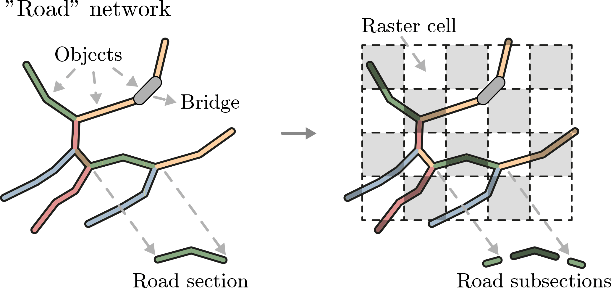
https://www.nat-hazards-earth-syst-sci.net/18/2273/2018/nhess-18-2273-2018-f03

Figure 3The road network consists of numerous objects. The objects considered are bridges and road sections, which are mapped as edges in the network. Given spatial considerations during the risk assessment, the road sections are divided into subsections. The length of subsections is defined by a projected raster grid matching the grid of the hazard events.

Download

With regards to determining the system representation, the analyzed events (organized using the generic categories introduced in Sect. 2) are presented next. It is worth noting that all events were described in terms of their spatial and temporal characteristics, and measures of the intensities were assigned to these events to describe attributes of interest. Once these events were defined, scenarios were built considering the relationships among events as suggested by the caption of Fig. 1.

Source event: rainfall, runoff.
Hazard events: floods and mudflows.
Object events: bridge local scour, road section inundation, road section mud-blocking, speed reduction, and capacity reduction.
Network events: network functionality.
Societal events: restoration interventions, traffic changes.

To model the spatio-temporal behavior of rainfall and the changes in river discharge values, a larger area than the area used for assessing the hazard events was considered for the source events. This is illustrated in Fig. 2. The hazard and object events were bounded to the corresponding catchment area of the region. The boundaries of the network and societal events exceeded the boundary of the object events to properly model the effects at the network level. The costs were only accounted for the Chur region. National-level impacts were not considered (e.g., blockade of the transit route from northern Europe to the south). Furthermore, scenarios were divided into time steps, with the duration of each time step varying, depending on the occurred events in the scenario. Source and hazard events were observed every hour, in order to account for gradual changes of the system (e.g., the traveling paths of rainfall, the increase of river stage). Object, network, and societal events were evaluated on an hourly basis during the hazard events and on a daily basis after the hazard events as the restoration time was expressed in working days.

3.3 Modules

Due to the modular approach of the simulation engine, events were represented as autonomous physical models grouped in modules, where only the metadata such as needed input and output had to be defined (a module can contain one or more models). Modules and models were developed in-house using Python to support the detailed study of (i) the behavior of the comprising models as the source code was available, and (ii) the uncertainties and propagation as all variables and functions of the individual models were known and could be modified. As most network managers use geographic information systems (GIS), a GIS data interface was developed to facilitate the import and export of data. Furthermore, the program code was optimized for massively parallel computing to reduce the computational time of the optimization process (i.e., each simulation ran on a designated CPU and thus an increase in the amount of CPUs increased the number of simulations for a given time frame). Brief descriptions of the modules used are provided in the following sections. For the interested reader, mathematical definitions of each module are given in the Supplement of this paper.

3.3.1 Rainfall

The experimental precipitation catalog described by Wüest et al. (2010) was used as the data source for rainfall modeling. The dataset covers all of Switzerland for the period between May 2003 and 2010. This catalog was derived from a combination of precipitation-gauge-based high-resolution interpolations and an hourly composite of radar measurements. The aggregation of the two data sources allowed for a catalog of very high resolution at the spatial scale (1 km²) and at the temporal scale (1 h). The initial precipitation fields were sampled from this catalog using randomized start hours and durations. The precipitation values for each raster cell for each time step were then scaled to associate the return period of a generated river discharge value at a location of interest with that of the rainfall (Hackl et al., 2017).

Inputs.: The return period desired to be investigated⁶.
Outputs.: A time series of precipitation fields (i.e., raster file for every time step), where the cell values represented the rainfall intensity per time step [mm h⁻¹]⁷.

3.3.2 Runoff

The modified Clark (ModClark) model by Kull and Feldman (1998) was used to estimate the runoff. After parsing a watershed into a uniform grid (matching that of the rainfall), this model used a linear quasi-distributed transformation method to estimate the runoff based on the Clark conceptual unit hydrograph (Clark, 1945). The method accounted for spatial differences in precipitation and losses (Paudel et al., 2009), allowing to model runoff translation and storage. The implementation of this model was calibrated by comparing the calculated values with measured values from the stream and precipitation gauging stations in the area.

Inputs.: A time series of precipitation fields, where the cell values represented the rainfall intensity per time step [mm h⁻¹].
Outputs.: Hydrographs for different sections of the rivers in the area of study, which were generated using the excess of cells located at the basin outlets [m³ s⁻¹].

3.3.3 Flood

A one-dimensional hydraulic model for gradually varied steady flow in an open channel network was implemented for the 31 km-section of the Rhine river in the area of study. This model was used to simulate the floodplain inundation by first computing the water surface profile of a given cross-section to the next, and then interpolating inundation values in between cross-sections to obtain the inundation field for the area of study. The 198 cross-sections, with an average distance of 150 m between them, were obtained from a digital elevation model (DEM) of the area. The model boundary conditions were represented by (i) the discharges at Ilanz and Fürstenau, (ii) the water level at the Rhine outlet, and (iii) the evolution of the additional discharges per cross-section derived from the computed hydrographs. The (Manning) roughness coefficients were estimated based on soil cover and land use. The hydraulic model was calibrated based on historical records of the stream gauging stations in the area.

Inputs.: Hydrographs for different sections of the rivers in the area of study [m³ s⁻¹].
Outputs.: A time series of inundation fields (i.e., raster file for every time step), where the cell values represented the floodwater depth above ground [m].

3.3.4 Mudflow

The mudflow model consisted of three main processes: (i) determination of potential mudflow locations, (ii) modeling the potential geometries and volumes, and (iii) estimation of the probability to trigger a mudflow. Potential locations and geometries were obtained from Losey and Wehrli (2013). Potential locations were determined using geological data and relief parameters as described in Giamboni et al. (2008), and geometries were calculated using the random walk routine of Gamma (2000). In total, 54 potential mudflows were considered in the target area of study. The volume of each mudflow was then estimated by calculating the runout length of the fan using the empirical relation of Rickenmann (1999). The increase in elevation per cell was calculated by dividing the mudflow volume by the area of the fan.

The probability of occurrence was estimated by first using the empirical intensity-duration function for sub-alpine regions proposed by Zimmermann et al. (1997) to determine which mudflows could be triggered at a given time step. When intensity-duration thresholds were exceeded at the site of a potential mudflow, a probability of being triggered was assigned to the mudflow event. This probability was related to the corresponding estimated slope factor of safety (Skempton and Delory, 1952). When determined to be triggered, the mudflow process was assumed to happen within one simulation time step.

Inputs.: A time series of precipitation fields, where the cell values represented the rainfall intensity per time step [mm h⁻¹].
Outputs.: A time series of mudflow fields (i.e., raster file for every time step), where the cell values represented the deposited mudflow volume [m³].

3.3.5 Object fragility

The relationships between hazard and object events were represented by fragility functions. These functions related hazard intensity measures Ξ, such as river discharge, inundation depth, and mudflow volume, to the likelihood of meeting or exceeding a determined damage (limit) state s of a bridge, road section/subsection. As fragility functions do not consider monetized consequences (as opposed to vulnerability functions⁸, which measure monetized consequence ratios), their use allows treating damages and their consequences separately. The fragility functions developed for this work were assumed to be log-normally distributed (Eq. 2), where S is the realization of the damage state, s is a possible damage state of an object, Ξ is the observed intensity measure of the hazard event at the object location, Φ denotes the standard normal cumulative distribution function, and μ and σ are the parameters of the estimated probability distribution.

\begin{matrix} (2) & P [S \geq s | Ξ] = Φ (\frac{\ln Ξ - μ}{σ}) \end{matrix}

The estimated damage state exceedance probabilities output considered the cumulative effects of hazard events. In other words, only the maximum hazard intensity measure observed up until a time step t was used at that time step to determine the damage state exceedance probabilities. The following subsections provide specific details on the development of the fragility functions for bridge local scour, road section inundation, and road section mud-blocking.

Bridge local scour

Assuming a negligible contraction of the riverbed cross-sections (Gehl and D'Ayala, 2015), only local (pier) scour was considered for the application, resulting in the selection of five bridges that could fail as a result of this phenomenon. To quantify different levels of local scour, four damage states were defined as described in Table 1. Fragility functions were used to relate these damage states with a range of possible river discharge values for bridges with one pier and those with two piers. The method used the local scour model of Arneson et al. (2012) and a Monte Carlo scheme to generate 100 000 uncertain local scour depths. These depths were compared with depth thresholds assumed to correspond to each damage state, leading to the estimation of damage state exceedance probabilities. The derived fragility parameters are given in Table 2. The fragility functions are illustrated in Fig. 4.

Table 1Damage states for bridge local scour, road section inundation and road section mud-blocking.

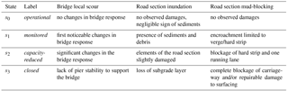
Download Print Version | Download XLSX

Table 2Fragility function parameters for bridge local scour, road section inundation and road section mud-blocking.

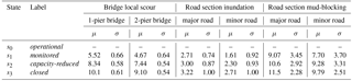
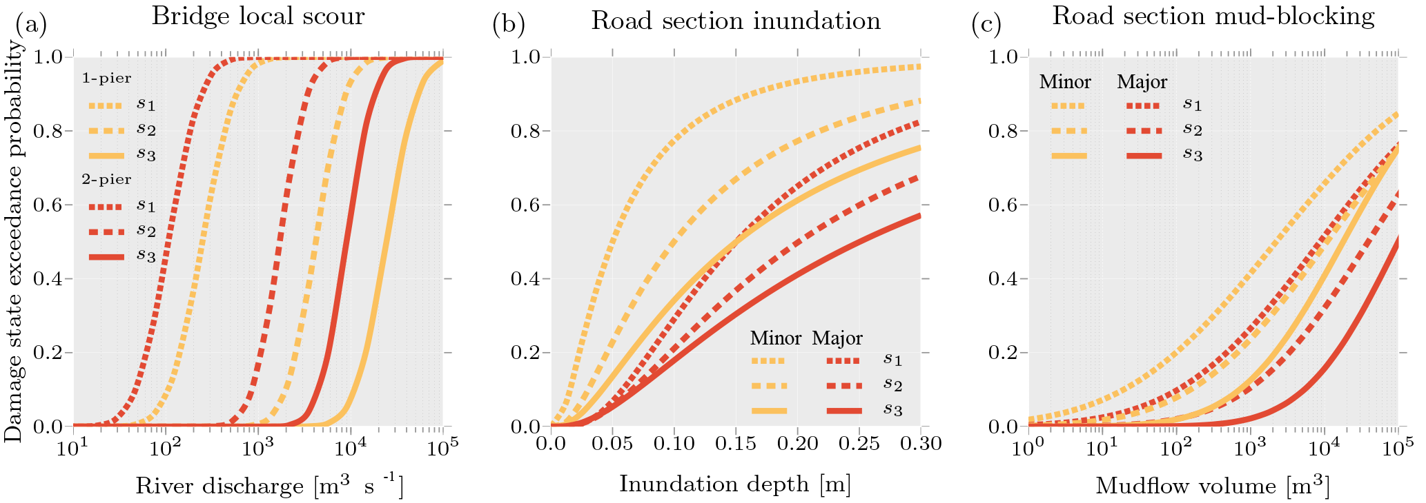
Download Print Version | Download XLSX

https://www.nat-hazards-earth-syst-sci.net/18/2273/2018/nhess-18-2273-2018-f04

Figure 4Fragility functions for (a) bridge local scour, (b) road section inundation, and (c) road section mud-blocking. The horizontal axis represents the intensity measure Ξ of the corresponding hazard. For (a) bridge local scour and (c) road section mud-blocking the axes are displayed in log-scale. The vertical axis represents the exceedance probabilities for the different damage states. The parameters μ and σ of these functions are given in Table 2.

Download

Road section inundation

The determination of the probable damages of a road section, whether part of a major or minor road, due to floods is an active field of research. The small amount of available data makes describing such relationship in a numerical form a challenging task. Some works (e.g., De Bruijin, 2005; Kok et al., 2005; Koks et al., 2012; Tariq et al., 2014; Li et al., 2016) have sought to numerically describe the relationship between damages and inundation depth. However, there are observed differences in the methods and results (e.g., some works bundled direct and indirect costs in their estimates), leading to the conclusion that these numerical relationships can only be applied to specific contexts and confined geographical areas.

To overcome this challenge, a different approach was taken, which involved proposing fragility functions based on data and information published by previous works seeking to qualitatively illustrate the impact of floods on road sections (e.g., ALA, 2005; ADEPT, 2011; Walsh, 2011; Vennapusa et al., 2013; Roslan et al., 2015). Despite the use of these studies, the proposed functions remain to be coarse illustrations that cannot be used in practice without further analysis. To qualify different levels of damage, four damage states were defined as described in Table 1. The fragility function parameters are given in Table 2. The fragility functions are displayed in Fig. 4.

Road section mud-blocking

To determine the level of road section mud-blocking, a distinction was made between high-speed (major) and local (minor) roads. The damage states defined by this work were based on the descriptions of Winter et al. (2013). These states are shown in Table 1. Fragility functions were estimated using expert data from the survey conducted by Winter et al. (2013), where experts were asked to relate debris flow volumes and damage state exceedance probabilities for different damage states and road categories (in doing so, it was here assumed that the results of this survey, focused on debris flow, could be used for determining a relationship between mudflows and road sections). The fragility function parameters are given in Table 2. The fragility functions are shown in Fig. 4.

Inputs.: (i) Hydrographs for different sections of the rivers in the area of study (out of which only those hydrographs for the river sections with the bridges of interest were selected during the analysis) [m³ s⁻¹], (ii) a time series of inundation fields, where the cell values represented the floodwater depth above ground [m], and (iii) a time series of mudflow fields, where the cell values represented the deposited mudflow volume [m³].
Outputs.: Time series of damage state exceedance probabilities considering cumulative damages for bridges due to local scour, road sections/subsections due to inundation, and road sections/subsections due to mud-blocking.

3.3.6 Object functionality

In terms of loss of functionality, a distinction was made between speed reduction and capacity reduction. The reduction of travel speed was used as a temporary measure during the hazard events period, indicating the drivers' response to the changed driving conditions (i.e., on an inundated road, drivers reduced their speed). In addition to this temporary measure, it was assumed that damages in objects would result in reduction of capacity (lane closure). In order to return to an adequate level of service, such objects had to be repaired (see Sect. 3.3.15).

Speed reduction

During the hazard events period, the relationship between inundation depths and feasible vehicle speeds on the road was derived from the data presented by Pregnolato et al. (2017). An exponential function was fitted to these data to describe the limit vehicle speed in a road as a function of inundation depth. The maximum acceptable velocity that ensures safe control of a vehicle through a specific section at a certain time when considering the inundation depth i was estimated by $v = v^{max} \cdot e^{- 0.10814 \cdot i}$ . Where v^max describes the maximum allowed speed on a road (e.g., 120 km h⁻¹). It was assumed that vehicles were only operated until an inundation depth of 0.3 m.

Capacity reduction

The relationships between the hazard events and the reduction in capacity were represented by functional loss functions (Lam and Adey, 2016). Expected functional losses were determined as functions of time-dependent hazard intensities Ξ, damage state s probabilities derived from fragility functions' damage state exceedance probabilities, and functional loss values λ associated with the investigated damage states (Eq. 3). The expected functional loss of a specific object at a specific time in the simulation is represented by $〈 λ 〉 \in [0, 1]$ .

\begin{matrix} (3) & 〈 λ 〉 = E (λ | Ξ) = \sum_{s} E (λ | s) \cdot P [S = s | Ξ] \end{matrix}

Table 3 presents the estimated loss values λ used. The values were either directly obtained or inferred from a survey conducted by D'Ayala and Gehl (2015). A loss value of λ=0 represents no reduction in capacity (i.e., all lanes are open) while a loss value of λ=1 indicates that no capacity is available (i.e., all lanes are closed). The functional loss functions are illustrated in Fig. 5.

Table 3Functional loss estimations for bridge local scour, road section inundation, and road section mud-blocking.

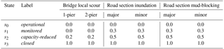
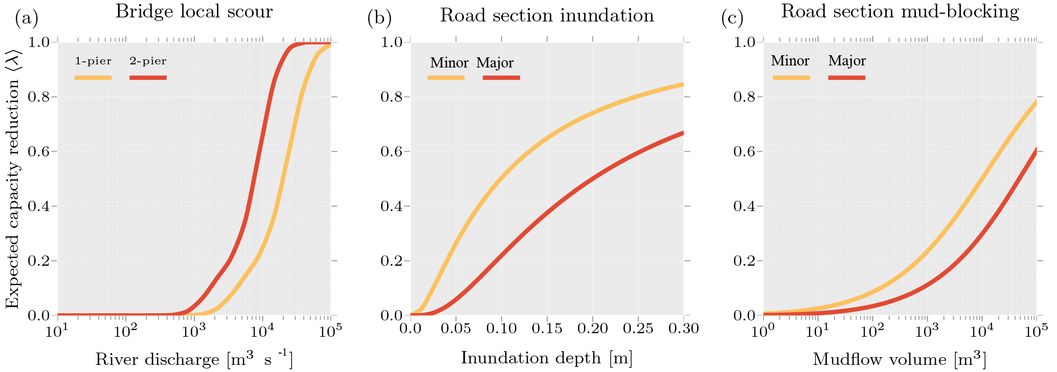
Download Print Version | Download XLSX

https://www.nat-hazards-earth-syst-sci.net/18/2273/2018/nhess-18-2273-2018-f05

Figure 5Functional loss functions for (a) bridge local scour, (b) road section inundation, and (c) road section mud-blocking. The horizontal axis represents the intensity measure Ξ of the corresponding hazard. For (a) bridge local scour and (c) road section mud-blocking the axes are displayed in log-scale. The vertical axis represents the expected functional loss.

Download

Inputs.: (i) A time series of inundation fields, where the cell values represented the floodwater depth above ground [m], and (ii) time series of damage state exceedance probabilities considering cumulative damages for bridges due to local scour, road sections/subsections due to inundation, and road sections/subsections due to mud-blocking.
Outputs.: (i) A time series of speed reduction for inundated road sections/subsections, and (ii) time series of expected capacity reduction for bridges with scoured piers, inundated road sections/subsections and mud-blocked road sections/subsections.

3.3.7 Object restoration needs

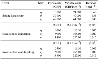
For each damaged bridge, road section/subsection, a restoration intervention had to be executed. Associated with each intervention were (i) the functional losses due to the execution of the intervention (i.e., functional loss during the restoration intervention), (ii) the length of time required to execute the intervention (i.e., restoration time), and (iii) the cost of the intervention (i.e., restoration cost). These values were estimated using the same convention as that of Eq. (3), where λ is replaced by the functional loss during the restoration intervention (in this application, these losses were assumed to be the same as those in Table 3), restoration times and restoration costs.

While a restoration cost was composed of a fixed part (e.g., site setup) and a variable part (e.g., CHF m⁻² of pavement, CHF m⁻³ of concrete, where mu stands for monetary units), the corresponding restoration time was approximated as a single value (i.e., no distinction between activities related to fixed and variable costs). These costs and durations are shown in Table 4. Cost estimates were based on Staubli and Hirt (2005) and from a survey conducted by D'Ayala and Gehl (2015). For each damage state, a restoration strategy was derived, and for each strategy, a restoration cost⁹ and a restoration time were approximated. It was assumed that the selected restoration program did not affect intervention costs.

Table 4Restoration costs and times for bridge local scour, road section inundation, and road section mud-blocking.

Download Print Version | Download XLSX

Inputs:: Time series of damage state exceedance probabilities considering cumulative damages for bridges due to local scour, road sections/subsections due to inundation, and road sections/subsections due to mud-blocking.
Outputs:: Time series of the expected capacity reduction during restoration intervention, restoration costs [CHF], and restoration times [h] for bridges with scoured piers, inundated road sections/subsections and mud-blocked road sections/subsections.

3.3.8 Network

In cases where a road section had to be split into subsections, assigned functional losses, restoration costs, and restoration times to subsections were aggregated to the section level. Aggregation routines of subsections' functional losses, restoration costs and restoration times were implemented, which assigned the maximum functional loss of subsections in a given section to that section and the sum of the restoration costs and the sum of the restoration times of subsections in a given section to that section. The routine corresponding to the estimation of functional losses is schematized in Fig. 6. As described in this figure as well, prior to this aggregation (from subsection level to section level) another aggregation had to be performed to consider the impact of the multiple time-varying hazard events. This latter estimation of functional losses, restorations costs, and times for subsections is described in Lam et al. (2018 b). The algorithm presented in Lam et al. (2018 b) is also applicable for bridges.

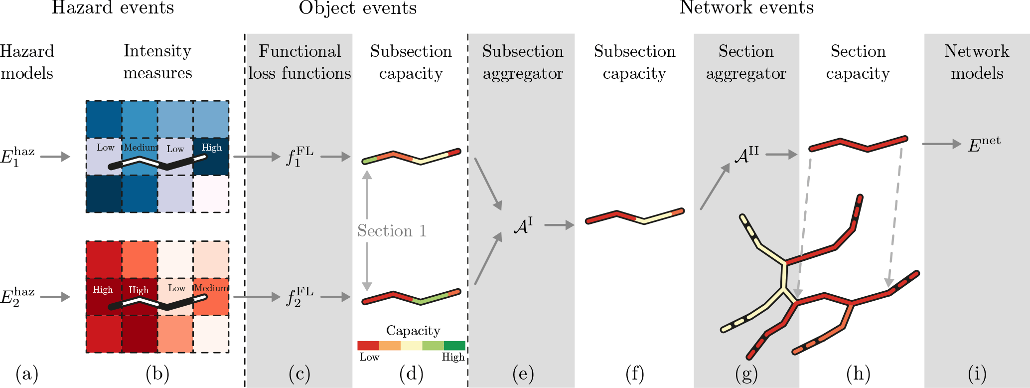
https://www.nat-hazards-earth-syst-sci.net/18/2273/2018/nhess-18-2273-2018-f06

Figure 6The hazard events (a) were represented in the form of a spatially distributed grid where the intensity measures change for each cell (b). Each road section of the network had to be split up according to this grid, which resulted in a set of subsections. This process was also previously illustrated in Fig. 3. In this specific example, the considered section is split into four subsections (b). The intensities are then processed independently for each of these subsections. For each intensity measure, the expected functional loss (i.e., speed reduction, capacity reduction) for each subsection is determined using computed functional loss functions $f_{1}^{FL}$ and $f_{2}^{FL}$ (c). Schematized in panel (d) are the resulting functional losses that are encoded in the colors of the subsections. A subsection aggregator 𝒜^I (e) is executed for each subsection and combines all functional loss values derived from different hazard events into a single value (f). This aggregator simply takes the maximum functional loss values. Finally, a section aggregator 𝒜^II (g) combines the functional losses of the subsections into a single functional loss for the section (h). Losses at the section level are then used in the network model (i). (This figure was adapted from Heitzler et al., 2018.)

Download

Once aggregated to the section level, functional losses, restoration costs, and restoration times for road sections, along with those for bridges, were assigned as attributes to the network. This required modeling the road network as a graph composed of 1520 vertices (i.e., 37 centroids, 1056 junctions, and 427 changes in road geometric features) and 3202 directed edges, where each edge represented a bridge or a road section. As the road network is located in a mountainous area, the topology of the network is such that certain areas are served by a single road, which means that, if part of this road is disrupted, there is no valid rerouting alternative and part of the demand remains unsatisfied. This results in missed trips. For this network, in particular, these edges (also referred to as cut links) represented about 11 % of the entire edge set.

After the hazard events period, the network was restored using a restoration model. This model supported the updating of damaged objects to restored objects (see Sect. 3.3.15), leading to updated network graphs to be used in the traffic model to estimate the indirect costs.

Inputs.: (i) A time series of speed reduction for inundated road sections/subsections; (ii) time series of expected capacity reduction for bridges with scoured piers, inundated road sections/subsections, and mud-blocked road sections/subsections; (iii) time series of the expected capacity reduction during restoration intervention, restoration costs [CHF], and restoration times [h] for bridges with scoured piers, inundated road sections/subsections, and mud-blocked road sections/subsections; and (iv) a restoration program, defining when each damaged object is to be restored.
Outputs.: (i) A time series of routable network graphs that can be used for traffic assignment; and (ii) time series of the expected capacity reduction during restoration intervention, restoration costs [CHF], and restoration times [h] for bridges with scoured piers, inundated road sections, and mud-blocked road sections.

3.3.9 Traffic

Vehicle travelers were assumed to behave according to the user equilibrium principle, which states that they choose a route from their origin to their destination that minimizes their travel cost. This means that the travel cost between each origin–destination pair is uniquely defined (Jenelius et al., 2006). This cost depends on the travel costs of all edges in an origin–destination path, which change with traffic flow. A stable state is reached only when no traveler can reduce his/her own costs of travel by unilaterally changing routes (Sheffi, 1985). Travel time was estimated using the formulation proposed by the Bureau of Public Roads (1964).

Regarding the demand model, the origin–destination matrix was estimated by a gravity model based on population density and was related to the number of vehicles on an average hourly and an average daily basis. This matrix was calibrated and updated using information of recent traffic counts along a set of edges. The study area was divided into 37 zones. Every internal centroid corresponded on average to an area of 15 km² with a population of about 1000.

To reduce computational complexity, only changes in route choices were considered within the risk assessment (i.e., travel demand was assumed to be inelastic). This was deemed a reasonable assumption as a large majority of the travel demand was caused by trips to work, which are made under normal circumstances. Therefore, changes in destination choices, mode choices, or trip frequencies were not considered. Moreover, it was assumed that the duration of network closures was long enough for all travelers to be aware of them so that a new user equilibrium could be reached.

Inputs.: A time series of routable network graphs that can be used for traffic assignment.
Outputs.: (i) A time series of traffic flow and travel time for each edge in the network, (ii) a time series of missed trips in the network, and (iii) a time series of damaged bridges and road sections that caused loss of connectivity.

3.3.10 Restoration

Once the discharge values along the river returned to normal conditions and no further damages to objects could occur, the impaired network was restored. A basic restoration model simulated this procedure (an improved version of the work of Lam and Adey, 2016). The prioritization of restoration activities was done by first restoring objects that caused loss of connectivity, and then restoring objects based on their average traffic volume (i.e., the average daily traffic volume for each object under normal conditions). It was assumed that 10 reconstruction crews could work simultaneously and each crew could at most be assigned to one object. For each day until the restoration was finished, the model updated the objects' states and executed the traffic model described to support the estimation of indirect costs during the restoration period. The restoration process ended once the network was completely restored.

Inputs.: (i) Time series of the expected capacity reduction during restoration intervention and restoration times [h] for bridges with scoured piers, inundated road sections, and mud-blocked road sections; and (ii) a time series of damaged bridges and road sections that caused loss of connectivity.
Outputs.: A restoration program, defining when each damaged object is to be restored.

3.3.11 Direct and indirect costs

The direct costs were estimated to be the sum of the direct costs for each intervention to be executed during the restoration period. These costs were actually accrued during the hazard events period as bridges and road sections were impacted by the hazard events (see Sect. 3.3.12). The direct costs were composed of a fixed part (e.g., side setup) and a variable path (e.g., CHF m⁻³ of pavement). The direct costs associated with each damage state are given in Table 4. The indirect costs were comprised of costs for the prolongation of travel time and costs due to a loss of connectivity. These costs were accrued during the hazard events period and the restoration period. The travel time costs were estimated based on the increased amount of time vehicles spent traveling. The Swiss Association of Road and Transport Experts (VSS, 2009 a) approximated the travel time cost per vehicle to be 23.29 CHF h⁻¹. In addition to considering the time factor, indirect costs also accounted for the costs of vehicle operation, which were incurred as a result of fuel consumption and vehicle maintenance. Based on the estimates of VSS (2009 b), the mean fuel price was approximated with 1.88 CHF L⁻¹ with a mean fuel consumption of 6.7 L $/ 100 \cdot$ veh km and the operating costs per vehicle without fuel consumption was assumed to be $14.39 CHF / 100 \cdot$ veh km. The costs due to a loss of connectivity were estimated based on the unsatisfied demand and the resulting costs due to missed trips. For every hour of delay of a trip, costs in the amount of 83.27 CHF were charged.

Inputs.: (i) A time series of the expected restoration costs [CHF] for bridges with scoured piers, inundated road sections, and mud-blocked road sections; (ii) a time series of traffic flow and travel time for each edge in the network; and (iii) a time series of missed trips in the network.
Outputs.: Time series of the estimated direct and indirect costs.

4 Results

The results section is organized in three subsections that present (i) the results of a single simulation run, (ii) the aggregation of results of multiple simulations with the same return period, and (iii) the results of multiple scenarios with multiple return periods.

4.1 Single scenario

Figure 7 shows the changes in a scenario due to a flood of 500 year return period. For this specific chain of events, the hazard events extended over a period of 18 h while the restoration period lasted 23 days (please note that while only two time steps are shown in this figure, the full system evolution is given in the Supplement).

https://www.nat-hazards-earth-syst-sci.net/18/2273/2018/nhess-18-2273-2018-f07

Figure 7Spatio-temporal representation of the system. The columns represent the investigated events, while the rows illustrate different time steps of the considered scenario. Time step 1 represents the beginning of the simulation with all elements at their initial state. Time step 10 illustrates the system state close to the peak of the flood. As observed, road sections were damaged by the flood, which resulted in functional losses and a change of traffic flow. In this scenario, people living in the northern part of the area were cut off from the rest of the network due to severely inundated roads.

Download

In this scenario, the rainfall started at hour 1 and ended at hour 10, with the maximum precipitation observed around hours 6 and 7. The precipitation moved from the northwestern part of the study area to southeastern part. At hour 6, parts of the motorway to Fürstenau were flooded, which led to a detour of the traffic through the village of Bonaduz. At hour 8, the motorway was flooded between Tamins and Domat/Ems, which interrupted the west–east connection in the valley. Traffic had to detour through Chur and drive south. Due to the lag runoff, the maximum extent of the flood was reached at hour 11. Most of the flood damage was caused in the western part of Chur, while in the northern part, only the motorway and several minor roads were flooded. Additionally, the triggering of a mudflow next to the village of Felsberg can be observed in hour 10, causing the blockage of two minor roads. This type of analysis is useful, to investigate the spatial and temporal evolution of the events. However, a single scenario cannot capture the uncertainties of the events. To overcome this issue, multiple scenarios with the same initial conditions (i.e., the same return period) can be performed.

4.2 Multiple scenarios with the same return period

Figure 8 illustrates the aggregated simulation results for 100 scenarios with 500 year return period. On the top left, the 25, 50, and 75-percentile precipitation fields are shown, with darker areas indicating more intense rainfall. The hazard events of interest are also presented, specifically the 5, 50 and 95-percentile of possible inundation depths as well as the location of possible mudflows color-coded according to their probability of occurrence. The expected discharge along the river is also illustrated in the graph. It can be observed that the 5, 50 and 95-percentile values were approximately 1690 m³ s⁻¹ at section 30. This value corresponded to the targeted river discharge value for a 500 year flood at the predefined gauging station located in that section. While the estimated direct costs are illustrated in Fig. 8, the indirect costs are not shown because these latter costs are a property of the whole system, and hence no clear spatial positions can be assigned to them.

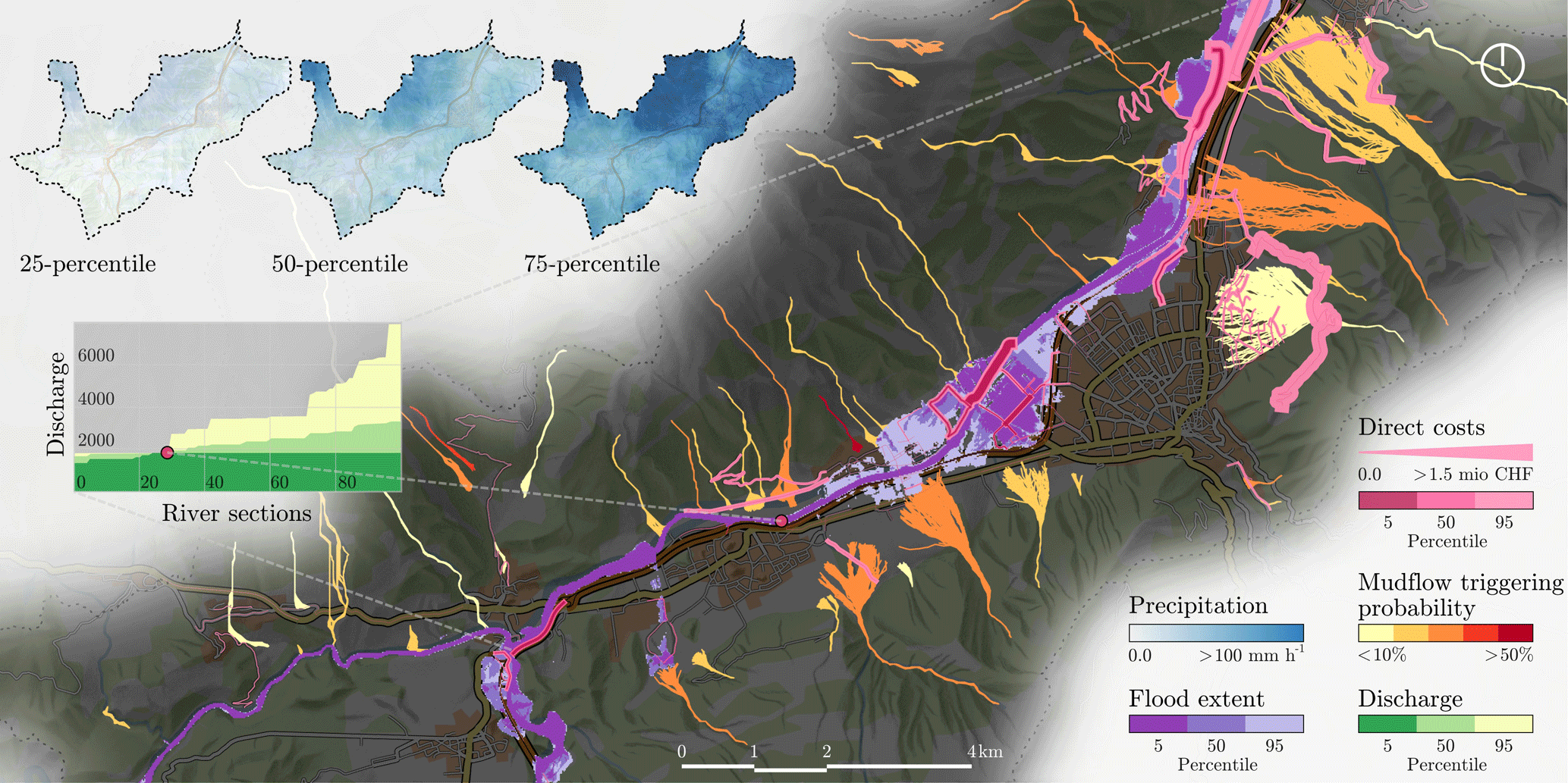
https://www.nat-hazards-earth-syst-sci.net/18/2273/2018/nhess-18-2273-2018-f08

Figure 8Aggregation of multiple simulations for hazard events with 500 year return period. This map visualizes the uncertainties related to these events. For example, only 5 % of the floods exceeded the light purple floodplain (95 % percentile), while only 5 % of the floods resulted in floodplains smaller than the dark purple area (5 % percentile).

Download

As illustrated in Fig. 8, the mapped floods can be interpreted as a probabilistic hazard map for events of a 500 year return period. While such maps can be used to reach some conclusions about the probable inundated areas, it is possible to also use geostatistical tools to analyze these and other information. Figure 9 shows the automatic cluster of damaged objects in the network using a mathematical algorithm that also supports the visualization of the associated direct costs. Such analysis can also be used for the planning of mitigation measures as part of the management of risk.

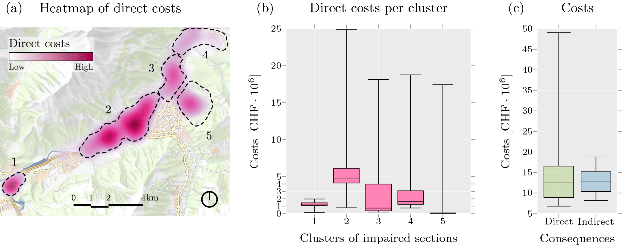
https://www.nat-hazards-earth-syst-sci.net/18/2273/2018/nhess-18-2273-2018-f09

Figure 9Direct and indirect costs related to the hazard events with 500 year return period. A heat map of expected direct costs for all scenarios (a) can be used to analyze high-risk areas. Here, five clusters were detected. The estimated direct costs per cluster and their associated uncertainties are illustrated in panel (b) using box plots. While in the second cluster, the median direct cost was around CHF 4.8 million, in the fifth cluster, a much smaller median value was estimated. However, the uncertainty of this cluster on the positive direction was comparable to that of the second cluster in the same direction. Comparing direct and indirect costs (c), their medians were similar. Nonetheless, the distribution of direct costs was positively skewed (heavy tail) while the distribution of indirect costs was close to symmetrical.

Download

Figure 9 gives additional insights on the resulting costs. Direct costs followed a heavy-tailed distribution (i.e., scattered high values in the positive direction of the distribution). Such distributions are often observed when considering extreme events, which is the case in the application that modeled random mudflows in addition to floods. For example, a mudflow was occasionally triggered in cluster five (see Figs. 8 and 9). When the mudflow was not triggered, little to no damage was observed in this cluster; however, when the mudflow was triggered, severe damage occurred. Contrary to direct costs, indirect costs followed a symmetric distribution due to the network redundancy (i.e., as long the network is not completely out of service, vehicles can take detours, leading to a redistributing of the indirect costs).

4.3 Multiple scenarios with multiple return periods

Figure 10 shows the obtained risk curves (return period vs. costs) with confidence intervals and annualized risk estimates (how much risk can be expected per year on average over a long period of time). Once a risk curve of a specific percentile was determined, its corresponding costs were used to estimate the matching annualized risk using Eq. (4) (Deckers et al., 2009), where ℛ^a is the annualized risk and C_i the costs associated with the annual exceedance probability $\frac{1}{T_{i}}$ , which is estimated based on the return period T of the event i. To use this equation, the events had to be arranged in decreasing order (e.g., $\frac{1}{2}, \frac{1}{5}, \dots, \frac{1}{10 000}$ ).

\begin{matrix} (4) & R^{a} = \sum_{i} \frac{1}{T_{i}} \cdot (C_{i} - C_{i - 1}) \end{matrix}

https://www.nat-hazards-earth-syst-sci.net/18/2273/2018/nhess-18-2273-2018-f10

Figure 10Risk curves and annualized risk estimations. The risk curves related to direct and indirect costs are illustrated in (a). The 50 % and 90 % confidence intervals are given for the sum of the costs. Costs associated with individual simulation runs are illustrated as gray dots. Equation (4) was used to calculate the annualized risk (b) for different cost percentiles. The median annualized risk for the sum of the costs was found to be CHF 2.4 million.

Download

When using this equation, direct costs were found to follow a heavy-tailed distribution. The median annualized risk related to direct consequences (CHF 1.5 million) was larger than that of indirect consequences (CHF 1 million). If other indirect consequences had been considered in addition to prolongation of travel time and missed trips (e.g., business interruptions), the annualized risk related to indirect consequences would be expected to increase significantly.

5 Discussion

As the main goal of the presented application was to illustrate the use of the methodology, models were selected based on the data available and a desire to keep computational time low to support the exploration of a large set of scenarios. This way, multiple hazards of various return periods could be considered along with changes in the traffic flow and restoration activities, leading to a more encompassing way to estimate risk. Due to the modular approach used, if desired, models that are more sophisticated may be integrated in the future. For example, the traffic model used here provided a low-complexity representation of driver behavior (e.g., travelers had full knowledge of the traffic conditions). Moreover, the traffic model did not account for dynamic phenomena like queues, spillbacks, wave propagation, or changes in travel patterns after a disruptive event (although studies show these can be considerably different after a disruptive event; e.g., Chang and Nojima, 2001; Kontou et al., 2017). In general, the integration of more sophisticated models can potentially lead to improved risk estimates. A prerequisite for this integration is conducting uncertainty and sensitivity analyses to prioritize the parts of the system to be analyzed in more detail.

Due to the modular approach and the universal nature of the models used, the implemented simulation engine conceptually can be used to estimate the risk related to other river systems and road networks, provided the required datasets are available. It is worth noting that the quantity and quality of data needed used in this study are largely available for many locations around the world. Alternatively, single parts of the simulation engine may be applied independently (e.g., to investigate the probability of bridge failure due to local scour at a given location). Hence, the system may be profitably used for a number of additional purposes (e.g., as a tool for cost-benefit analysis of flood and mudflow protection measures, as a decision support system for operational flood and mudflow control). As implemented, the risk assessment can provide a mechanism for a region-wide screening of priority locations for risk reduction based on the analysis of the road network and traffic properties (e.g., Heitzler et al., 2017). This function can be enhanced with the use of visualization tools, enabling network managers to dynamically see how different environmental systems (i.e., rainfall, flood and mudflow) influence each other, and how their impact on networks can affect society (Heitzler et al., 2016).

Finally, combining several models results in a significant degree of uncertainty. Whenever possible, the results should be compared with and calibrated against empirical data, when available. For example, the probability of damages obtained through simulations could be calibrated against collected data from field structural surveys when such data exist. Calibration for societal events is rather difficult because such data are difficult to measure and monitor. Nonetheless, in some cases, basic data are available, including the duration of a network's loss of functionality and the estimated number of network users affected.

6 Conclusions

The purpose of estimating the risk related to networks is, among others, to provide an overview of the probable adverse events that may negatively affect the network, assess their societal effects (e.g., costs), and provide a basis for planning risk-reducing interventions. Assessing the risk related to networks exposed to multiple types of hazards is not trivial due to the large number of events that need to be modeled in an integrated manner, their uncertainties and the propagation of these uncertainties affecting risk estimates. This is particularly evident when dealing with complex system representations, where the costs of indirect consequences can be multiple times higher than the costs of direct consequences, with no linear relationship between these types of cost.

This paper describes a risk assessment methodology for networks when there is a need to represent the system containing these networks using various degrees of complexity. The methodology is supported by a modular simulation engine that fosters multidisciplinary collaboration. Following this methodology, a state of the art application was designed and implemented, which aimed at estimating the spatio-temporal risk of a road network in Switzerland due to the occurrence of a time-varying rainfall that caused flood and mudflow events. To achieve this objective, the modular simulation engine was used to couple rainfall, runoff, flood, mudflow, damages, functional losses, traffic, and restoration modeling. Consequences were monetized into direct and indirect costs, considering restoration interventions, prolongation of travel time, and missed trips. The costs of the 1200 scenarios simulated were analyzed at three different levels: (i) those of a single simulation, (ii) those of multiple simulations with the same return period, and (iii) those of multiple simulations of multiple return periods. This number of scenarios supported the analysis of cost uncertainties.

The use of the methodology is not limited to hydro-meteorological hazard events or road networks. For example, the methodology can be applied to other hazards (e.g., earthquakes, coastal floods, rockfalls) or other networks (e.g., railway, waterways, inter-modal). Such analyses would require appropriate hazard models and descriptors of the relationships between the hazard events, damage, and functional losses (e.g., no rail traffic due to a settlement of the rail tracks following an earthquake), as well as appropriate datasets. Additionally, other societal events, such as business interruption, rescue missions, and access to education/health services, among others, could be implemented in future work. Nonetheless, depending on the complexity of the system representation, some of these applications may result in computationally intensive risk assessment designs, increasing the time required to compute risk estimates. However, for the simulation engine to be of value to other researchers it is necessary to refactor and clean up the code base.

Data availability

Special emphasis was put on using open data wherever possible. Data sets used are as follows: the geodata for Grisons can be found at the geographic information system of the canton of Grisons, accessible via https://geogr.ch/ (last access: 16 July 2018). Topographic data such as the administrative borders of the municipalities of Switzerland, aerial imagery and digital height model, from the whole of Switzerland were provided by https://www.swisstopo.admin.ch/ (last access: 16 July 2018) and obtained from https://opendata.swiss/ (last access: 16 July 2018). The Swiss flood and landslide damage database (Unwetterschadens-Datenbank) are provided to official institutions on request, by the Swiss Federal Institute for Forest, Snow and Landscape Research (https://www.wsl.ch/, last access: 16 July 2018). Detailed information about the data used in this paper is available upon request.

Supplement

The supplement related to this article is available online at: https://doi.org/10.5194/nhess-18-2273-2018-supplement.

Competing interests

The authors declare that they have no conflict of interest.

Acknowledgements

The work presented here has received funding from the European Union's Seventh Programme for Research, Technological Development and Demonstration under grant agreement no. 603960, and from Horizon 2020, the European Union's Framework Programme for Research and Innovation, under grant agreement no. 636285.

Edited by: Sven Fuchs
Reviewed by: two anonymous referees

References

ADEPT: Climate Change and Evolved Pavements, CSS Research Project 78, Association of Directors of Environment, Economy, Planning and Transport, 2011. a

Adey, B. T., Hackl, J., Lam, J. C., Van Gelder, P., Prak, P. P., Van Erp, N., Heitzler, M., Iosifescu-Enescu, I., and Hurni, L.: Ensuring acceptable levels of infrastructure related risks due to Nat. Hazards with emphasis on conducting stress tests, in: 1st International Symposium on Infrastructure Asset Management (SIAM2016), edited by: Kobayashi, K., Tamura, K., and Kaito, K., 19–29, Kyoto University, Kyoto, Japan, 2016. a

ALA: Flood-Resistant Local Road Systems: A Report Based on Case Studies, Report, American Lifelines Alliance, Washington, DC, USA, 2005. a

Apel, H., Thieken, A. H., Merz, B., and Blöschl, G.: Flood risk assessment and associated uncertainty, Nat. Hazards Earth Syst. Sci., 4, 295–308, https://doi.org/10.5194/nhess-4-295-2004, 2004. a

Arneson, L., Zevenbergen, L., Lagasse, P., and Clopper, P.: Evaluating Scour at Bridges Fifth Edition, Tech. Rep. 18, Federal Highway Administration, Washington, DC, USA, 2012. a

Berdica, K.: An introduction to road vulnerability: What has been done, is done and should be done, Transp. Policy, 9, 117–127, https://doi.org/10.1016/S0967-070X(02)00011-2, 2002. a

Bezzola, G. R. and Hegg, C.: Ereignisanalyse Hochwasser 2005, Teil 1 – Prozesse, Schäden und erste Einordnung, Umwelt-Wissen 0707.215 S, Bundesamt für Umwelt BAFU, Eidgenössische Forschungsanstalt WSL, Basel, Switzerland, 2007. a

Bocchini, P. and Frangopol, D. M.: Restoration of Bridge Networks after an Earthquake: Multicriteria Intervention Optimization, Earthq. Spectra, 28, 426–455, https://doi.org/10.1193/1.4000019, 2012. a

Bowering, E. A., Peck, A. M., and Simonovic, S. P.: A flood risk assessment to municipal infrastructure due to changing climate part I: methodology, Urban Water J., 11, 20–30, https://doi.org/10.1080/1573062X.2012.758293, 2014. a, b

Brunner, G. W.: HEC-RAS, River Analysis System: Hydraulic Reference Manual, Technical Report CPD-69, US Army Corps of Engineers Hydrologic Engineering Center (HEC), Davis, CA, USA, 2016. a

Bureau of Public Roads: Traffic Assignment Manual, Manual, Urban Planning Division, US Department of Commerce, Washington, DC, USA, 1964. a

Chang, S. E. and Nojima, N.: Measuring post-disaster transportation system performance: the 1995 Kobe earthquake in comparative perspective, Transport. Res. A.-Pol., 35, 475–494, https://doi.org/10.1016/S0965-8564(00)00003-3, 2001. a

Clark, C. O.: Storage and the unit hydrograph, T. Am. Soc. Civ. Eng., 110, 1419–1446, 1945. a

Dawson, R. J., Peppe, R., and Wang, M.: An agent-based model for risk-based flood incident management, Nat. Hazards, 59, 167–189, https://doi.org/10.1007/s11069-011-9745-4, 2011. a

D'Ayala, D. and Gehl, P.: Single Risk Analysis, Deliverable 3.4, Novel indicators for identifying critical, INFRAstructure at RISK from Natural Hazards (INFRARISK), University College London, London, UK, 2015. a, b

De Bruijin, K. M.: Resilience and flood risk management: A sytems approach applied to lowland rivers, PhD thesis, TU Delft, Delft, the Netherlands, 2005. a

Deckers, P., Kellens, W., Reyns, J., Vanneuville, W., and De Maeyer, P.: A GIS for Flood Risk Management in Flanders, in: Geospatial Techniques in Urban Hazard and Disaster Analysis, edited by: Showalter, P. S. and Lu, Y., vol. 2 of Geotechnologies and the Environment, 51–69, Springer Netherlands, Dordrecht, the Netherlands, https://doi.org/10.1007/978-90-481-2238-7_4, 2009. a, b

Dueñas-Osorio, L. and Vemuru, S. M.: Cascading failures in complex infrastructure systems, Struct. Saf., 31, 157–167, https://doi.org/10.1016/j.strusafe.2008.06.007, 2009. a

Eidsvig, U. M. K., Kristensen, K., and Vangelsten, B. V.: Assessing the risk posed by natural hazards to infrastructures, Nat. Hazards Earth Syst. Sci., 17, 481–504, https://doi.org/10.5194/nhess-17-481-2017, 2017. a

Elsawah, H., Guerrero, M., and Moselhi, O.: Decision Support Model for Integrated Intervention Plans of Municipal Infrastructure, ICSI 2014, 7, 1039–1050, https://doi.org/10.1061/9780784478745.098, 2014. a

Ferlisi, S., Cascini, L., Corominas, J., and Matano, F.: Rockfall risk assessment to persons travelling in vehicles along a road: the case study of the Amalfi coastal road (southern Italy), Nat. Hazards, 62, 691–721, https://doi.org/10.1007/s11069-012-0102-z, 2012. a

Fuchs, S. and Bründl, M.: Damage Potential and Losses Resulting from Snow Avalanches in Settlements of the Canton of Grisons, Switzerland, Nat. Hazards, 34, 53–69, https://doi.org/10.1007/s11069-004-0784-y, 2005. a

Fuchs, S. and Keiler, M.: Variability of Natural Hazard Risk in the European Alps: Evidence from Damage Potential Exposed to Snow Avalanches, in: Disaster Management Handbook, edited by: Pinkowski, J., vol. 138, chap. 13, 267–279, Taylor & Francis Group, Boca Raton, Florida, USA, https://doi.org/10.1201/9781420058635.ch13, 2008. a

Fuchs, S., Keiler, M., Sokratov, S., and Shnyparkov, A.: Spatiotemporal dynamics: the need for an innovative approach in mountain hazard risk management, Nat. Hazards, 68, 1217–1241, https://doi.org/10.1007/s11069-012-0508-7, 2013. a

Fuchs, S., Röthlisberger, V., Thaler, T., Zischg, A., and Keiler, M.: Natural Hazard Management from a Coevolutionary Perspective: Exposure and Policy Response in the European Alps, Ann. Am. Assoc. Geogr., 107, 382–392, https://doi.org/10.1080/24694452.2016.1235494, 2017. a

Gallina, V., Torresan, S., Critto, A., Sperotto, A., Glade, T., and Marcomini, A.: A review of multi-risk methodologies for Nat. Hazards: Consequences and challenges for a climate change impact assessment, J. Environ. Manage., 168, 123–132, https://doi.org/10.1016/j.jenvman.2015.11.011, 2016. a

Gamma, P.: dfwalk – Ein Murgang Simulationsprogramm zur Gefahrenzonierung, PhD thesis, University Bern, Bern, Switzerland, 2000. a

Gehl, P. and D'Ayala, D.: Integrated multi-hazard framework for the fragility analysis of roadway bridges, in: Proceedings of the 12th International Conference on Applications of Statistics and Probability in Civil Engineering (ICASP12), Vancouver, Canada, 12–15 July, edited by: Haukaas, T., p. 8, University of British Columbia Library, Vancouver, Canada, https://doi.org/10.14288/1.0076190, 2015. a

Giamboni, M., Wehrli, A., and Losey, S.: Simulation von gravitativen Naturgefahren für das Schutzwaldmanagement in der Schweiz: Das Projekt Silvaprotect-CH, Bulletin fuer Angewandte Geologie, 13, 83–95, https://doi.org/10.5169/seals-226686, 2008. a

Hackl, J. and Adey, B. T.: Generation of Spatially Embedded Random Networks to Model Complex Transportation Networks, in: 14th International Probabilistic Workshop, edited by: Caspeele, R., Taerwe, L., and Proske, D., Springer International Publishing, Cham, 217–230, https://doi.org/10.1007/978-3-319-47886-9_15, 2017. a

Hackl, J., Adey, B. T., Heitzler, M., and Iosifescu-Enescu, I.: An Overarching Risk Assessment Process to Evaluate the Risks Associated with Infrastructure Networks due to Nat. Hazards, International Journal of Performability Engineering, 11, 153–168, 2015. a

Hackl, J., Heitzler, M., Lam, J. C., Adey, B. T., and Hurni, L.: Development of flood and mudflow events for the spatio-temporal risk assessment of networks, European Water, 57, 197–203, 2017. a

Hammond, M., Chen, A., Djordjević, S., Butler, D., and Mark, O.: Urban flood impact assessment: A state-of-the-art review, Urban Water J., 12, 14–29, https://doi.org/10.1080/1573062X.2013.857421, 2015. a

He, X. and Liu, H. X.: Modeling the day-to-day traffic evolution process after an unexpected network disruption, Transport. Res. B.-Meth., 46, 50–71, https://doi.org/10.1016/j.trb.2011.07.012, 2012. a

Heitzler, M., Hackl, J., Adey, B. T., Iosifescu-Enescu, I., Lam, J. C., and Hurni, L.: A method to visualize the evolution of multiple interacting spatial systems, ISPRS J. Photogramm., 117, 217–226, https://doi.org/10.1016/j.isprsjprs.2016.03.002, 2016. a

Heitzler, M., Lam, J. C., Hackl, J., Adey, B. T., and Hurni, L.: GPU-Accelerated Rendering Methods to Visually Analyze Large-Scale Disaster Simulation Data, Journal of Geovisualization and Spatial Analysis, 1, 1–18, https://doi.org/10.1007/s41651-017-0004-4, 2017. a

Heitzler, M., Lam, J. C., Hackl, J., Adey, B. T., and Hurni, L.: A Simulation and Visualization Environment for Spatio- Temporal Disaster Risk Assessments of Network Infrastructures, Cartographica: The International Journal for Geographic Information and Geovisualization, 52, 349–363, https://doi.org/10.3138/cart.52.4.2017-0009, 2018. a, b

Hilker, N., Badoux, A., and Hegg, C.: The Swiss flood and landslide damage database 1972–2007, Nat. Hazards Earth Syst. Sci., 9, 913–925, https://doi.org/10.5194/nhess-9-913-2009, 2009. a

Jenelius, E., Petersen, T., and Mattsson, L. G.: Importance and exposure in road network vulnerability analysis, Transport. Res. A.-Pol., 40, 537–560, https://doi.org/10.1016/j.tra.2005.11.003, 2006. a, b, c

Keiler, M., Knight, J., and Harrison, S.: Climate change and geomorphological hazards in the eastern European Alps, Philos. T. Roy. Soc. A., 368, 2461–2479, https://doi.org/10.1098/rsta.2010.0047, 2010. a

Kok, M., Huizinga, H. J., Vrouwenvelder, A., and Barendregt, A.: Standaardmethode 2004 – Schade en Slachtoffers als gevolg van overstromingen, Tech. Rep. DWW-2005-005, Ministerie van Verkeer en Waterstaat, Utrecht, the Netherlands, 2005. a

Koks, E., De, H., and Koome, E.: Comparing Extreme Rainfall and Large-Scale Flooding Induced Inundation Risk – Evidence from a Dutch Case-Study, in: Studies on Water Management Issues, edited by: Kumarasamy, M., London, UK, chap. 1, 3–26, InTech, https://doi.org/10.5772/30378, 2012. a

Komendantova, N., Mrzyglocki, R., Mignan, A., Khazai, B., Wenzel, F., Patt, A., and Fleming, K.: Multi-hazard and multi-risk decision-support tools as a part of participatory risk governance: Feedback from civil protection stakeholders, Int. J. Disast. Risk. Re., 8, 50–67, https://doi.org/10.1016/j.ijdrr.2013.12.006, 2014. a, b

Kontou, E., Murray-Tuite, P., and Wernstedt, K.: Duration of commute travel changes in the aftermath of Hurricane Sandy using accelerated failure time modeling, Transport. Res. A.-Pol., 100, 170–181, https://doi.org/10.1016/j.tra.2017.04.015, 2017. a

Kull, D. W. and Feldman, A. D.: Evolution of Clark's Unit Graph Method to Spatially Distributed Runoff, J. Hydrol. Eng., 3, 9–19, https://doi.org/10.1061/(ASCE)1084-0699(1998)3:1(9), 1998. a

Lam, J. C. and Adey, B. T.: Functional Loss Assessment and Restoration Analysis to Quantify Indirect Consequences of Hazards, ASCE-ASME Journal of Risk and Uncertainty in Engineering Systems, Part A: Civil Engineering, 2, 04016008, https://doi.org/10.1061/AJRUA6.0000877, 2016. a, b, c

Lam, J. C., Adey, B. T., Heitzler, M., Hackl, J., Gehl, P., van Erp, N., D'Ayala, D., van Gelder, P., and Hurni, L.: Stress tests for a road network using fragility functions and functional capacity loss functions, Reliab. Eng. Syst. Safe., 173, 78–93, https://doi.org/10.1016/j.ress.2018.01.015, 2018a. a

Lam, J. C., Heitzler, M., Hackl, J., Adey, B. T., and Hurni, L.: Modelling the functional capacity losses of networks exposed to hazards, Sustainable and Resilient Infrastructure, Taylor & Francis, 1–19, https://doi.org/10.1080/23789689.2018.1469357, 2018b. a, b

Li, C., Cheng, X., Li, N., Du, X., Yu, Q., and Kan, G.: A Framework for Flood Risk Analysis and Benefit Assessment of Flood Control Measures in Urban Areas, Int. J. Env. Res. Pub. He., 13, 787, https://doi.org/10.3390/ijerph13080787, 2016. a

Losey, S. and Wehrli, A.: Schutzwald in der Schweiz: Vom Projekt SilvaProtect-CH zum harmonisierten Schutzwald, Final report, Bundesamt für Umwelt (BAFU), Bern, Switzerland, 2013. a

Mattsson, L.-G. and Jenelius, E.: Vulnerability and resilience of transport systems – A discussion of recent research, Transport. Res. A.-Pol., 81, 16–34, https://doi.org/10.1016/j.tra.2015.06.002, 2015. a

Merz, B., Kreibich, H., Schwarze, R., and Thieken, A.: Review article “Assessment of economic flood damage”, Nat. Hazards Earth Syst. Sci., 10, 1697–1724, https://doi.org/10.5194/nhess-10-1697-2010, 2010. a, b

Mignan, A., Wiemer, S., and Giardini, D.: The quantification of low-probability-high-consequences events: part I, A generic multi-risk approach, Nat. Hazards, 73, 1999–2022, https://doi.org/10.1007/s11069-014-1178-4, 2014. a, b

Paudel, M., Nelson, E. J., and Scharffenberg, W.: Comparison of Lumped and Quasi-Distributed Clark Runoff Models Using the SCS Curve Number Equation, J. Hydrol. Eng., 14, 1098–1106, https://doi.org/10.1061/(ASCE)HE.1943-5584.0000100, 2009. a

Pellicani, R., Argentiero, I., and Spilotro, G.: GIS-based predictive models for regional-scale landslide susceptibility assessment and risk mapping along road corridors, Geomat. Nat. Haz. Risk., 5705, 1–22, https://doi.org/10.1080/19475705.2017.1292411, 2017. a, b

Pregnolato, M., Ford, A., Wilkinson, S. M., and Dawson, R. J.: The impact of flooding on road transport: A depth-disruption function, Transport. Res. D.-Tr. E., 55, 67–81, https://doi.org/10.1016/j.trd.2017.06.020, 2017. a

Pritchard, O. G., Hallett, S. H., and Farewell, T. S.: Soil geohazard mapping for improved asset management of UK local roads, Nat. Hazards Earth Syst. Sci., 15, 2079–2090, https://doi.org/10.5194/nhess-15-2079-2015, 2015. a

Rickenmann, D.: Empirical Relationships for Debris Flows, Nat. Hazards, 19, 47–77, https://doi.org/10.1023/A:1008064220727, 1999. a

Roslan, N. I., Ghani, A. N. A., and Hamid, A. H. A.: Road subgrade strength under various flooding event, Jurnal Teknologi, 75, 39–43, 2015. a

Rupi, F., Bernardi, S., Rossi, G., and Danesi, A.: The Evaluation of Road Network Vulnerability in Mountainous Areas: A Case Study, Networks and Spatial Economics, 15, 397–411, https://doi.org/10.1007/s11067-014-9260-8, 2015. a, b, c

Scawthorn, C., Flores, P., Blais, N., Seligson, H., Tate, E., Chang, S., Mifflin, E., Thomas, W., Murphy, J., Jones, C., and Lawrence, M.: HAZUS-MH Flood Loss Estimation Methodology I: Overview and Flood Hazard Characterization, Nat. Hazards Review, 7, 72–81, https://doi.org/10.1061/(ASCE)1527-6988(2006)7:2(72), 2006. a

Schlögl, M. and Laaha, G.: Extreme weather exposure identification for road networks – a comparative assessment of statistical methods, Nat. Hazards Earth Syst. Sci., 17, 515–531, https://doi.org/10.5194/nhess-17-515-2017, 2017. a

Shabou, S., Ruin, I., Lutoff, C., Debionne, S., Anquetin, S., Creutin, J.-D., and Beaufils, X.: MobRISK: a model for assessing the exposure of road users to flash flood events, Nat. Hazards Earth Syst. Sci., 17, 1631–1651, https://doi.org/10.5194/nhess-17-1631-2017, 2017. a

Sheffi, Y.: Urban transportation networks: equilibrium analysis with mathematical programming methods, Prentice-Hall, Englewood Cliffs, NJ, USA, 1985. a

Skempton, A. W. and Delory, F. A.: Stability of Natural Slopes in London Clay, Thomas Telford Publishing, London, UK, 378–381, https://doi.org/10.1680/sposm.02050.0011, 1952. a

Staubli, R. and Hirt, T.: Werterhalt von Strassen, Leitfaden für Politiker und Praktiker 1, Schweizerischer Gemeindeverband, Urtenen-Schönbühl, Switzerland, 2005. a

Suarez, P., Anderson, W., Mahal, V., and Lakshmanan, T. R.: Impacts of flooding and climate change on urban transportation: A systemwide performance assessment of the Boston Metro Area, Transport. Res. D.-Tr. E., 10, 231–244, https://doi.org/10.1016/j.trd.2005.04.007, 2005. a

Tariq, M., Hoes, O., and Van de Giesen, N.: Development of a risk-based framework to integrate flood insurance, J. Flood Risk. Manag., 7, 291–307, https://doi.org/10.1111/jfr3.12056, 2014. a

Taubenböck, H., Goseberg, N., Lämmel, G., Setiadi, N., Schlurmann, T., Nagel, K., Siegert, F., Birkmann, J., Traub, K. P., Dech, S., Keuck, V., Lehmann, F., Strunz, G., and Klüpfel, H.: Risk reduction at the ”Last-Mile”: An attempt to turn science into action by the example of Padang, Indonesia, Nat. Hazards, 65, 915–945, https://doi.org/10.1007/s11069-012-0377-0, 2013. a

Taylor, M. and D'Este, G.: Transport Network Vulnerability: a Method for Diagnosis of Critical Locations in Transport Infrastructure Systems, in: Critical Infrastructure, edited by: Murray, A. and Grubesic, T., Advances in Spatial Science, Springer Berlin Heidelberg, 9–30, https://doi.org/10.1007/978-3-540-68056-7_2, 2007. a

Thacker, S., Pant, R., and Hall, J. W.: System-of-systems formulation and disruption analysis for multi-scale critical national infrastructures, Reliab. Eng. Syst. Safe., 167, 30–41, https://doi.org/10.1016/j.ress.2017.04.023, 2017. a

Vennapusa, P. K. R., White, D. J., and Miller, D. K.: Western Iowa Missouri River Flooding – Geo-Infrastructure Damage Assessment, Repair and Mitigation Strategies, Tech. Rep. September, Center for Earthworks Engineering Research, Ames, IA, USA, 2013. a

Vespignani, A.: Complex networks: The fragility of interdependency, Nature, 464, 984–985, https://doi.org/10.1038/464984a, 2010. a

Vetsch, D., Siviglia, A., Ehrbar, D., Facchini, M., Gerber, M., Kammerer, S., Peter, S., Vanzo, D., Vonwiller, L., Volz, C., Farshi, D., Mueller, R., Rousselot, P., Veprek, R., and Faeh, R.: System Manuals of BASEMENT, Manual Version 2.8, Laboratory of Hydraulics, Glaciology and Hydrology (VAW), Zurich, Switzerland, 2018. a

VSS: Kosten-Nutzen-Analysen im Strassenverkehr: Zeitkosten im Personenverkehr, Swiss Standard SN 641 822a, Swiss Association of Road and Transport Experts (VSS), Zurich, Switzerland, 2009a. a

VSS: Kosten-Nutzen-Analysen im Strassenverkehr: Betriebskosten von Strassenfahrzeugen, Swiss Standard SN 641 827, Swiss Association of Road and Transport Experts (VSS), Zurich, Switzerland, 2009b. a

Vugrin, E. D., Turnquist, M. A., and Brown, N. J. K.: Optimal recovery sequencing for enhanced resilience and service restoration in transportation networks, International Journal of Critical Infrastructures, 10, 218–246, https://doi.org/10.1504/IJCIS.2014.066356, 2014. a

Walsh, I.: The Effects of Inundation on Pavements, Report 383, Jacobs, London, UK, 2011. a

Wang, Z., Chan, A. P. C., Yuan, J., Xia, B., Skitmore, M., and Li, Q.: Recent Advances in Modeling the Vulnerability of Transportation Networks, J. Infrastruct. Syst., 21, 1–9, https://doi.org/10.1061/(ASCE)IS.1943-555X.0000232, 2014. a

Winter, M., Smith, J., Fotopoulou, S., Pitilakis, K., Mavrouli, O. C., Corominas Dulcet, J., and Argyroudis, S.: The physical vulnerability of roads to debris flows, in: International Symposium on Landslides, Taylor and Francis Group, Banff, 307–313, 2013. a, b

Wüest, M., Frei, C., Altenhoff, A., Hagen, M., Litschi, M., and Schär, C.: A gridded hourly precipitation dataset for Switzerland using rain-gauge analysis and radar-based disaggregation, Int. J. Climatol., 30, 1764–1775, https://doi.org/10.1002/joc.2025, 2010. a

Zimmermann, M., Mani, P., and Gamma, P.: Murganggefahr und Klimaänderung – ein GIS-basierter Ansatz, NFP 31 Schlussbericht, vdf, Hochsch.-Verlag an der ETH, Zurich, Switzerland, 1997. a

Numerous definitions for network vulnerability have been proposed in the literature. In most cases, the literature has defined network vulnerability in terms of the effects of service disruption, irrespective of its probability (Berdica, 2002; Taylor and D'Este, 2007; Wang et al., 2014). In the context of the present work, vulnerability is defined in the same terms, acknowledging that it is an inherent attribute of any network and thus an essential element of risk assessments.

A more detailed overview of the canton of Grisons and its damage potential against natural hazards can be found in Fuchs and Bründl (2005).

WSL Unwetterschadens-Datenbank der Schweiz.

⁴

Events that caused damage to buildings or forestry/agricultural assets are not considered here.

⁵

A definition of these terms can be found in Hilker et al. (2009).

⁶

The term “inputs” refers to those inputs that are provided by other modules in the simulation engine, or externally by the network manager.

⁷

The term “outputs” refers to those outputs that are provided by the module and can be used by all other modules, or ultimately can be regarded to be the estimated consequences.

⁸

Such functions are also referred to as damage functions and loss functions.

⁹

Costs taken from the literature were adjusted to 2017 price levels. To avoid over interpreting the specific values that were in the application, monetary units are used instead of real currency.

Articles

Download

Article (4114 KB)
Full-text XML

Short summary

This paper introduces a methodology to support network managers in the quantification of the risk related to their networks. The method emphasizes the integration of the spatial and temporal attributes of the events that need to be modeled to estimate the risk. This work then demonstrates the usefulness of the methodology through its application to design and implement a risk assessment to estimate the potential impact of flood and mudflow events on a road network located in Switzerland.