the Creative Commons Attribution 4.0 License.
the Creative Commons Attribution 4.0 License.
 | 29 Aug 2018
Combining temporal 3-D remote sensing data with spatial rockfall simulations for improved understanding of hazardous slopes within rail corridors
Megan van Veen
D. Jean Hutchinson
David A. Bonneau
Zac Sala
Matthew Ondercin
Matt Lato
Remote sensing techniques can be used to gain a more detailed understanding of hazardous rock slopes along railway corridors that would otherwise be inaccessible. Multiple datasets can be used to identify changes over time, creating an inventory of events to produce magnitude–frequency relationships for rockfalls sourced on the slope. This study presents a method for using the remotely sensed data to develop inputs to rockfall simulations, including rockfall source locations and slope material parameters, which can be used to determine the likelihood of a rockfall impacting the railway tracks given its source zone location and volume. The results of the simulations can be related to the rockfall inventory to develop modified magnitude–frequency curves presenting a more realistic estimate of the hazard. These methods were developed using the RockyFor3D software and lidar and photogrammetry data collected over several years at White Canyon, British Columbia, Canada, where the Canadian National (CN) Rail main line runs along the base of the slope. Rockfalls sourced closer to the tracks were more likely to be deposited on the track or in the ditch, and of these, rockfalls between 0.1 and 10 m3 were the most likely to be deposited. Smaller blocks did not travel far enough to reach the bottom of the slope and larger blocks were deposited past the tracks. Applying the results of the simulations to a database of over 2000 rockfall events, a modified magnitude–frequency can be created, allowing the frequency of rockfalls deposited on the railway tracks or in ditches to be determined. Suggestions are made for future development of the methods including refinement of input parameters and extension to other modelling packages.


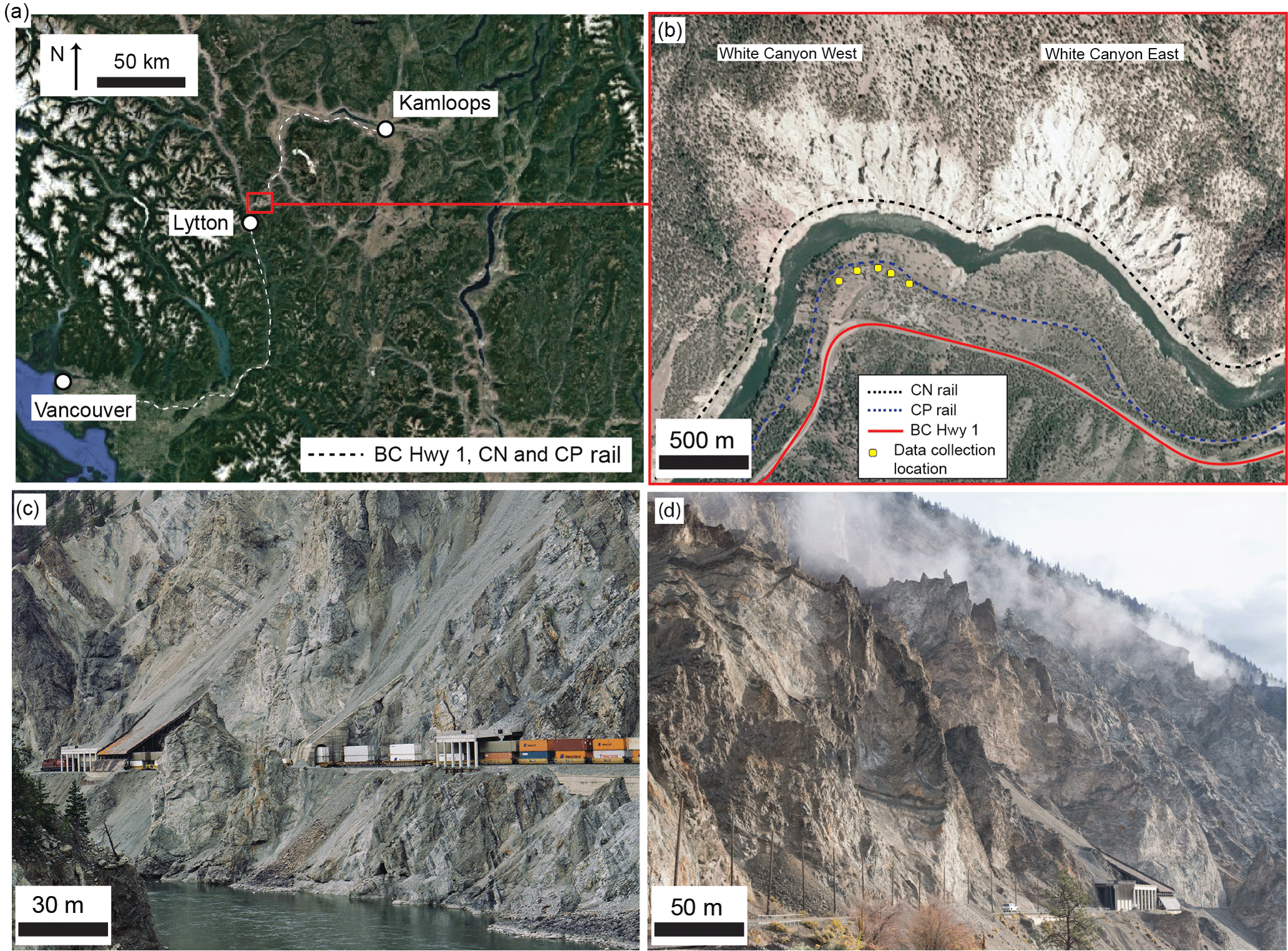
Figure 1(a) Location of the White Canyon. (b) Plan view of the White Canyon West and East slopes with the location of highway and rail lines indicated. Panels (c) and (d) Photographs of the White Canyon West illustrating complex geometry formed by deeply incised talus channels and vertical outcrops. Rock sheds are located at the base of several talus channels to guide material over the railway tracks.
Railways in western Canada are subject to frequent rockfall hazards, which can be evaluated using remotely sensed data, derived from lidar or structure from motion (SfM) photogrammetry. Often, these technologies provide advantages over traditional methods of data collection on steep and inaccessible slopes, such as the ability to identify rockfall release points, which can be a large source of uncertainty in developing rockfall magnitude–frequency relationships (Corominas et al., 2018). Change detection performed between sequential lidar scans can be used to identify and characterize rockfall source zones and develop magnitude–frequency relationships for a slope (Rosser et al., 2005; Santana et al., 2012; D'Amato et al., 2013; Guerin et al., 2014; van Veen et al., 2017). These inventories can contain a greater level of detail for rockfalls in the smaller volume ranges relative to traditional field inspections performed from the base of the slope (Dussauge-Peisser et al., 2002); however, it is often difficult to determine the trajectory or ending point of each event, which is affected by the slope materials and geometry, and the characteristics of the failed block, including its lithology (Deere and Miller, 1966). While many have demonstrated the ability to develop rockfall magnitude–frequency relationships using remote sensing data, these inventories likely overestimate the likelihood of a block interacting with critical infrastructure at the base of a slope. Evaluation of rockfall trajectories can provide insight into the potential behaviour of rockfalls, which can be used, along with the magnitude–frequency and rockfall source zone information, in refining the hazard assessment for a given section of railway. Along with the locations and characteristics of rockfall source zones, remote sensing data can also provide us with detailed surface models for use in rockfall modelling environments. The use of 2.5-D and 3-D environments for computer based rockfall modelling provides advantages over traditional 2-D methods, as the entire slope can be examined without having to draw cross-sections through selected areas and model along only those paths (Lan et al., 2010; Ondercin et al., 2014).
1.1 Study objectives
This study investigates how detailed remote sensing data of multiple types can be incorporated into rockfall simulations, to create representative surface models and to develop input parameters for rockfall source zones and slope characteristics. The input parameters extracted from the remote sensing data include rockfall sources and source zone characteristics (ex. lithology, slope angle) in addition to detailed slope classifications used to assign material properties. We compare several different cases based on rockfall volumes and source zone locations using RockyFor3D, a widely available industry standard 2.5-D point mass model (Dorren, 2015). We present a method that uses the results of the rockfall simulations to determine the likelihood of a rockfall impacting the railway tracks given its volume and source zone location. These results can be used to modify the magnitude–frequency curves for rockfall source zones (developed using lidar data) to develop a more refined estimate of the hazard likelihood.
1.2 Study site
The site of interest is known as the White Canyon, and is located approximately 250 km northeast of Vancouver, near the town of Lytton, BC (Fig. 1). The CN Rail line runs along the base of the slope, which is separated into two sections by a short tunnel, White Canyon West and East. The work presented in this paper focuses on the White Canyon West section. Due to differential weathering of several lithological units, the canyon contains many deeply incised channels, which are actively transporting debris downslope predominantly by dry granular flows and debris flows (Bonneau and Hutchinson, 2017). Surrounding these channels are areas of more competent rock outcrop, which act as source zones for rockfall. Many of these areas contain large vertical spires, contributing to the complex geometry of the slope (Fig. 1) and affecting the passage of rockfalls from higher source elevations to the railway tracks or into the river at the bottom of the slope. For this reason, the ability to model rockfalls on this slope in more than two dimensions is advantageous.
The slope is composed of a highly fractured and foliated quartzofeldspathic gneiss with a series of tonalite dykes and dioritic intrusions. A section of red-stained and highly weathered granodiorite from the Mt. Lytton Batholith is also present in a small section of the slope (Brown, 1981). The degree of fracturing is variable throughout the canyon, leading to a variety of rockfall block shapes and sizes within each unit. The amount of weathering is also variable across the slope, and affects the behaviour of rockfalls.
The high frequency of rockfalls on this slope presents a challenge to the rail operators. Typically, track-level assessments by CN Rail provide records that can be added to a database of rockfall events for a given slope and rail corridor. These could include events that have directly impacted the track or blocks that are noted in ditches adjacent to the rail. Using CN's Rockfall Hazard Rating System (RHRA, Abbott et al., 1998b), events are categorized into three volume classes based on the largest block dimension at track level (less than 0.3 m, 0.3 to 1.0 m, and greater than 1.0 m). Of these sizes, the blocks between 0.3 and 1.0 m in size present the greatest concern as they are the size most likely to become wedged under a train, lifting it off the tracks and causing a derailment (Abbott et al., 1998a). Smaller blocks may not present as significant of a hazard and larger blocks are more likely to set off rockfall warning systems such as trip wire fences. For slopes where activity is frequent, such as the White Canyon, these inspection-based databases are often incomplete as it is difficult to identify individual small events that may occur between inspections as a single rockfall.
As a part of the Canadian Railway Ground Hazards Research Program, remote sensing data, including terrestrial laser scanning (TLS), airborne laser scanning (ALS) and SfM photogrammetry data, have been collected at the site since 2012. Several studies have been completed using this data with details outlined in Hutchinson et al. (2015), Kromer et al. (2015), van Veen et al. (2017) and Rowe et al. (2018). By performing change detection between sequential lidar scans, we have constructed a detailed database of rockfall events in the canyon for the time period between November 2014 and May 2016 (18 months).
Data were collected over a period of 18 months for the White Canyon West slopes. The data was processed to create models of the full slope, which were classified to develop inputs to the rockfall simulations. Change detection methods were used to extract rockfall event information from the data and develop rockfall magnitude–frequency curves for the analysis period.
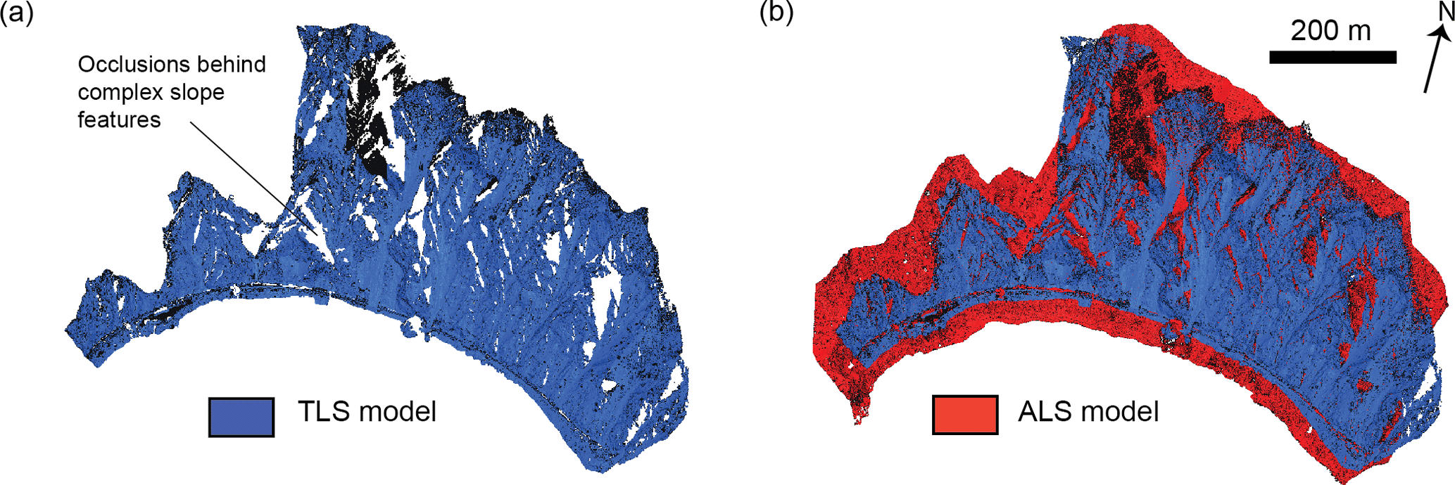
Figure 2(a) Plan view of TLS model for the White Canyon West slopes. (b) Plan view of aligned TLS and ALS models for the White Canyon West slopes.
2.1 Remote sensing data collection and creation of slope models
The TLS data for the White Canyon West slopes used in this study were collected on eight dates between November 2014 and May 2016. The duration between collection dates ranged from 1 to 4 months and was dependent on site access and weather conditions. Data were collected using an Optech ILRIS-3D scanner from five different sites on the opposite bank of the Thompson River (Fig. 1). The survey was designed such that there was significant overlap between sites, in order to minimize the amount of data occluded from the overall slope model. TLS data were collected at a distance of 300 to 700 m from the slope with an average point spacing of 10 cm. ALS data (point spacing ranging from 30–60 cm) were collected in October of 2015, 1 week prior to a TLS data collection campaign, and was provided by CN Rail.
Sequential TLS datasets can be aligned to one another by picking common points between the models and then performing an iterative closest point (ICP) alignment (Besl and McKay, 1992). A single slope model was created for each of the eight TLS scan dates by combining the data from each of the five individual scan sites. Each completed TLS model was aligned to the baseline reference model collected in November 2014. Due to the complex geometry of the slope, both the TLS and ALS data contain occlusions; however, combination of both models provides near-complete coverage of the slope. In order to create a single model of the slope to be used as a modelling surface, the ALS data were aligned to the TLS data from October 2015 (datasets collected approximately 1 week apart). The resulting slope model is shown in Fig. 2. The result of this process is a point cloud model of the slope with reduced occlusions compared to the TLS model on its own.
A set of overlapping photos of the slope was collected on 11 September 2013 using a Canon 6D camera with a 50 mm lens. The 94 photos were used to create a photogrammetric model of the slope using Agisoft PhotoScan Pro (Agisoft, 2015) with a point spacing of 10–20 cm. This model was aligned to the lidar reference model using the same methods described above.
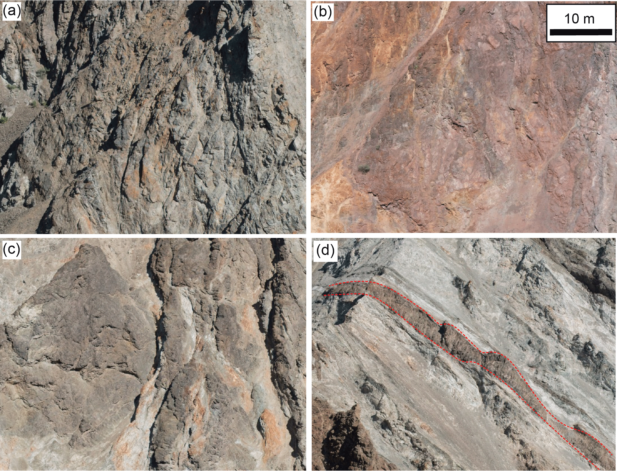
Figure 3Examples of the four main geological units in the White Canyon. (a) Quartzofeldspathic gneiss (Lytton Gneiss); (b) red-stained granodiorite (Mt. Lytton Batholith); (c) dioritic intrusions and (d) tonalite dyke (outlined in red).
2.2 Classification of slope models
The slope was classified into each of the four major lithological units present using the photogrammetric model (Fig. 3): Quartzofeldspathic Gneiss (primary rock type), Mt. Lytton Batholith (granodiorite), tonalite dykes, and dioritic intrusions. This classification was performed though visual inspection and tracing of each outcrop area on the 3-D model using the methods and preliminary work developed by Jolivet et al. (2015) as described in van Veen et al. (2016). The same process was used to separate the slope into areas of rock outcrop (potential rockfall source zones) and areas of soil and talus, and to classify the slope by visual assessment of the Geological Strength Index (GSI) (Marinos and Hoek, 2000). GSI values were assigned by visually comparing high-resolution photographs of the rock mass with the GSI characterization table for jointed rock. Sections of the rock mass were assigned a GSI value based on the rock mass structure and conditions of discontinuities observed on the outcrop surface. The classified slope model for each of the categories described above is shown in Fig. 4.

Figure 4Classified slope models for White Canyon West based on: (a) lithology; (b) ground cover type and (c) GSI. White spaces represent occlusions in the model.
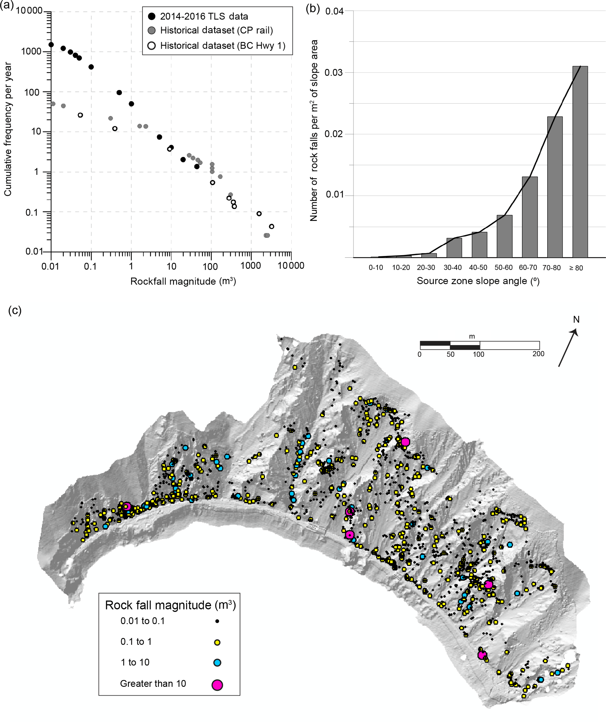
Figure 5(a) Magnitude–cumulative-frequency curves for rockfalls extracted from TLS compared to historical records (digitized from Hungr et al., 1999). (b) Graph of rockfall frequencies based on source zone slope angles. (c) Spatial distribution of rockfall event locations from TLS data collected between 11 November 2014 and 2 May 2016.
2.3 Extraction of rockfall magnitude–frequency and source zone information
Rockfall locations and volumes were extracted from the TLS change detection using 3-D point-based methods and spatial clustering algorithms as described in van Veen et al. (2017). A limit of detection threshold of 0.05 m was applied based on the alignment error between sequential TLS datasets and additional noise filters were applied during data processing. Results were validated using high-resolution photos collected simultaneously with the TLS data. Using the rockfall locations, each event could also be related to its source zone lithology and GSI using the classified models, as well as the source zone slope angle for each event. We created an inventory of events, using the eight TLS datasets that were collected between November 2014 and May 2016 (18 months). This inventory was used to produce a magnitude–cumulative-frequency (MCF) curve and spatial distribution plot for the rockfalls on the slope during this time period (Fig. 5). While a short time period of only 18 months may not be sufficient to establish magnitude–frequency relationships for larger rockfall events, it provides enough detail to understand the smaller magnitude hazards, which affect the day-to-day operation of the railway.
Hungr et al. (1999) compiled a rockfall inventory over the previous four decades along the Canadian Pacific rail line and BC Highway 1 corridor from Vancouver to Kamloops. The CP line generally follows the same route as CN throughout this corridor but is located on the opposite bank of the Thompson and Fraser rivers. These historical records contain data for events where volume information was available and span magnitudes from 0.01 to 3000 m3 with a noted under-sampling of events below 1 m3. While this inventory can not be directly compared to the inventory generated using TLS, due to the different sampling periods and variation in route of the railways and highways, the TLS analysis methods provide a higher level of detail for rockfalls in the range of 0.01 to 1 m3 compared to the historical inventory for this area. In addition to a higher level of detail for smaller volume ranges, the rockfall information gathered from lidar provides information on the location of rockfall source zones, which can be used to characterize the failure processes operating on the slope. This information is not available from historical records collected at the base of a slope.
The RockyFor3D model (Dorren, 2015) is a 2.5-D point mass model used to calculate rockfall trajectories as 3-D vector data. RockyFor3D is an industry standard software model that utilizes GIS data formats for model inputs, outputs and visualization. This model was used to simulate rockfalls ranging from 0.01 to 100 m3 across the entire slope of the White Canyon West. The classified slope models were used to determine input parameters for the RockyFor3D modelling. The results of these models allowed us to determine the percentage of the simulated rockfalls that landed in the ditch at the base of the slope, on the railway tracks or past the tracks for a given source zone location and volume.
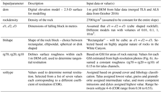
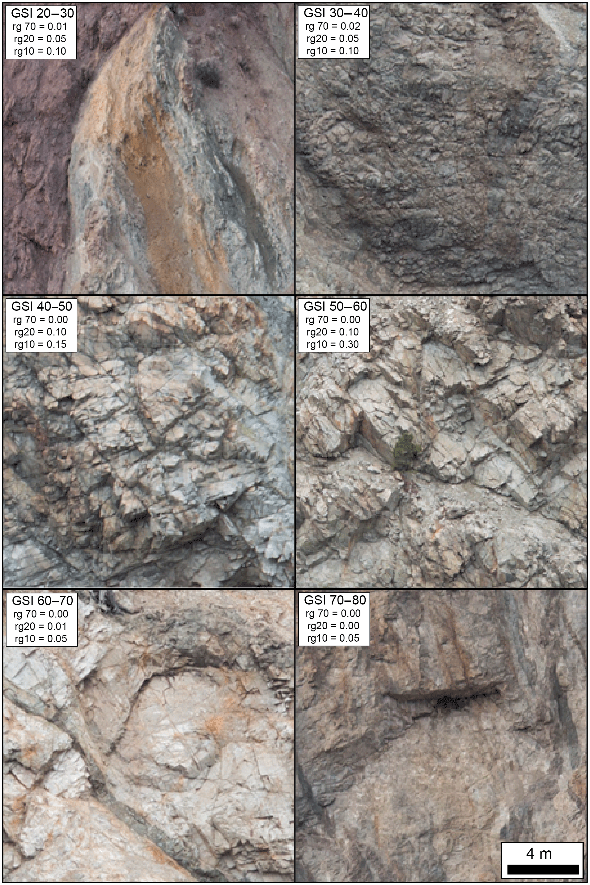
Figure 6Examples of slope areas for each of the classified GSI ranges. The rg70, rg20 and rg10 input parameters to the RockyFor3D model for each GSI class are indicated. The 20–30 and 30–40 GSI examples are shown from the Mt. Lytton Batholith. All other images are the quartzofeldspathic gneiss unit.
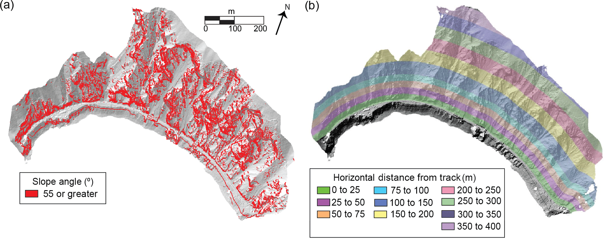
Figure 7(a) Rockfall source zones used in RockyFor3D modelling, based on slope angle. (b) Horizontal distances from track used for modelling to relate deposited blocks to their source zone.
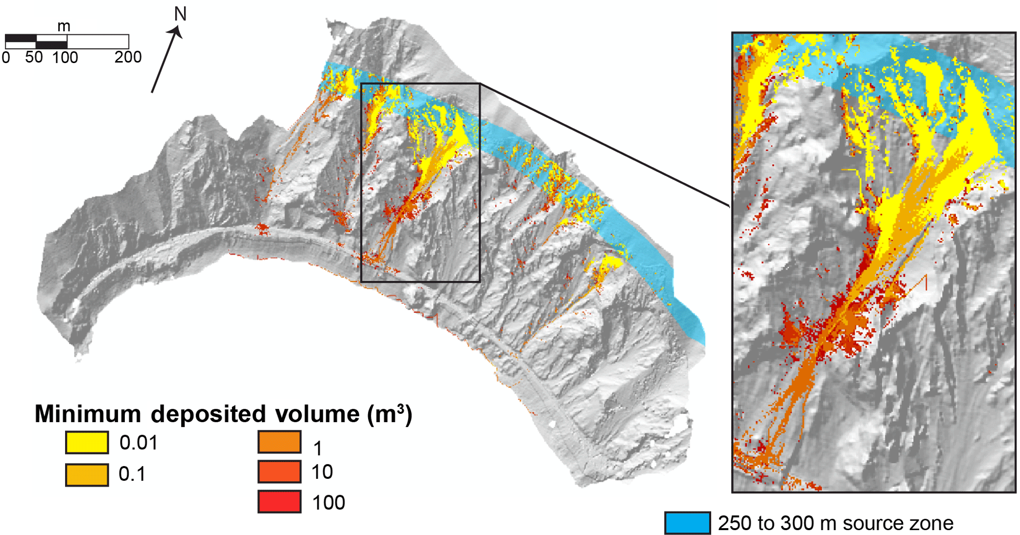
Figure 8Example of deposition outputs from the RockyFor3D model for the 250 to 300 m source zone. Coloured cells indicate rockfall deposition points and the colour of the cell represents the minimum volume deposited in each cell: for example, the darkest red colour represents cells in which only blocks 100 m3 were deposited, and the second darkest colour represents cells in which blocks 10 m3 or larger (100 m3 were deposited).
3.1 Input parameters
The RockyFor3D model requires 10 different input parameters which are summarized in Table 1. The Digital Elevation Model (DEM) was created from the merged TLS–ALS dataset from the canyon using an inverse distance weighted interpolation in ArcGIS and the rg70, rg20, rg10 and soiltype parameters were estimated based on the classified slope models. The rg70, rg20 and rg10 parameters represent the “roughness” of the slope within each DEM cell by specifying the height of obstacles that a rockfall will encounter within each 1 m cell of the DEM in 70 %, 20 % and 10 % of cases (Dorren, 2015). The surface roughness parameters for areas of rock outcrop were estimated based on the GSI classification for each slope area (Fig. 6).
3.2 Modelling process
The four different rockfall volumes, ranging from 0.01 to 10 m3 were sourced from grid cells where the slope angle exceeded 55∘ (Fig. 5). The threshold of 55∘ was selected based on an analysis of the slope angle at known rockfall source points (Fig. 5). When comparing the number of rockfalls per unit area of different slope angle ranges, there was a distinct increase in the relative rate of rockfalls for slope angles between 50–60∘ and greater. While it may be argued that this increase occurs at a larger angle, a conservative approach was taken, given the relatively short time period used to produce this dataset. The rockfall source zones were selected using this logic as opposed to sourcing only from known rockfall event locations (within the 18-month period) as to better capture all of the potential source zones on the slope. At each source zone cell, 500 blocks were sourced. One model was run for each volume category and source distance from the railway track (total of 40 models, Fig. 7). Smaller zones (25 m distance increments) were used for the first 100 m and 50 m buffered contours were used for distances greater than 100 m, such that the results would contain more detail for rockfalls occurring closer to the tracks.
3.3 Results
The results from the RockyFor3D simulations were combined and used to produce raster maps of rockfall deposition locations for each of the source zone distance ranges, an example of which is shown in Fig. 8. These raster maps display the minimum volume that was deposited in each cell based on the simulations. Any block larger than the size shown can also be deposited in these locations, thus showing the minimum volume allows for an understanding of the full range of block sizes that could be deposited in each location. The rockfall deposition points were classified and used to determine the percentage of rockfalls being deposited in a given location based on the assumptions made for the model inputs. The deposition percentages were split into rockfalls deposited in the ditch, on the railway tracks, below track level and the percentage remaining on the slope for each volume and source distance (Fig. 9). The general trends observed in the deposition results are summarized in Table 2.
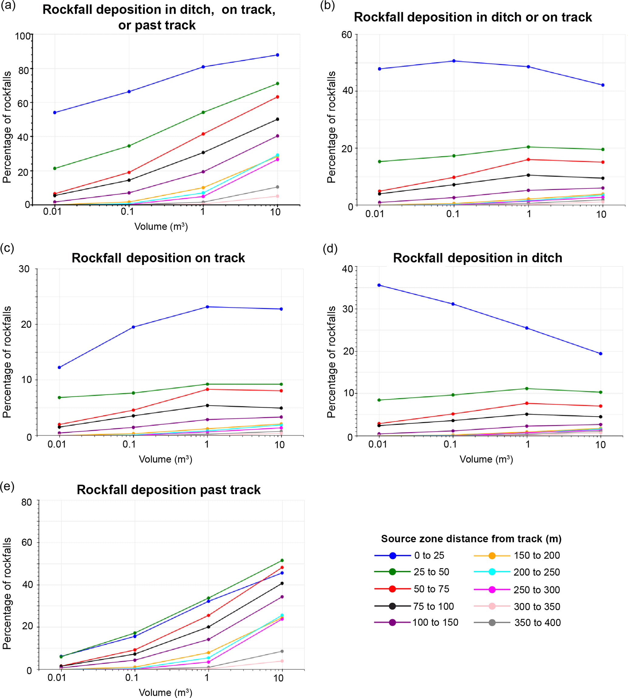
Figure 9Rockfall deposition percentages based on classified outputs from the RockyFor3D model showing (a) percentage of rockfalls deposited in the ditch, on tracks, or past the tracks, (b) in the ditch or on the tracks, (c) on the tracks, (d) in the ditch and (e) past the tracks (on the downslope side).
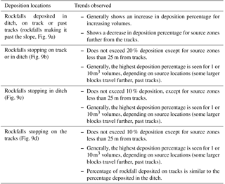
Table 2Summary of trends observed from RockyFor3D modelling deposition results.
For rockfall source zones less than 25 m from the tracks, the percentage of events deposited in the ditch or on the tracks was 20 % to 30 % higher than rockfalls sourced at larger distances. In the lower sections of the slope, there are fewer complex geometrical features and fewer zones of talus present, which provides a more direct passage for rockfalls to be deposited on or near the tracks. Smaller volumes were more likely to be deposited in the ditches than larger volumes, and the 1 and 10 m3 blocks were most likely to be deposited on the tracks. It is possible that the local slope roughness does impact the results, and that there may be certain areas of the slope where the roughness or slope angles play a larger role than others; however, the distance from the track appears to be the controlling factor in the overall percentage of rockfalls making it to track level. For rockfalls sourced from the uppermost slopes, the results show that a larger percentage of blocks sourced from 350 to 400 m are reaching the base of the slope compared to blocks sourced from 300 to 350 m. This result occurs because there are relatively few potential source zones between 350 and 400 m. Due to where these source zones are located, a larger proportion of the blocks travel further, compared to the 300–350 distance where there is a larger spatial variation in source zones, and the slope geometry has more of an overall effect. The total number of simulated blocks sourced from 300–350 reaching the base of the slope is larger than 350–400; however, the relative proportion is smaller.
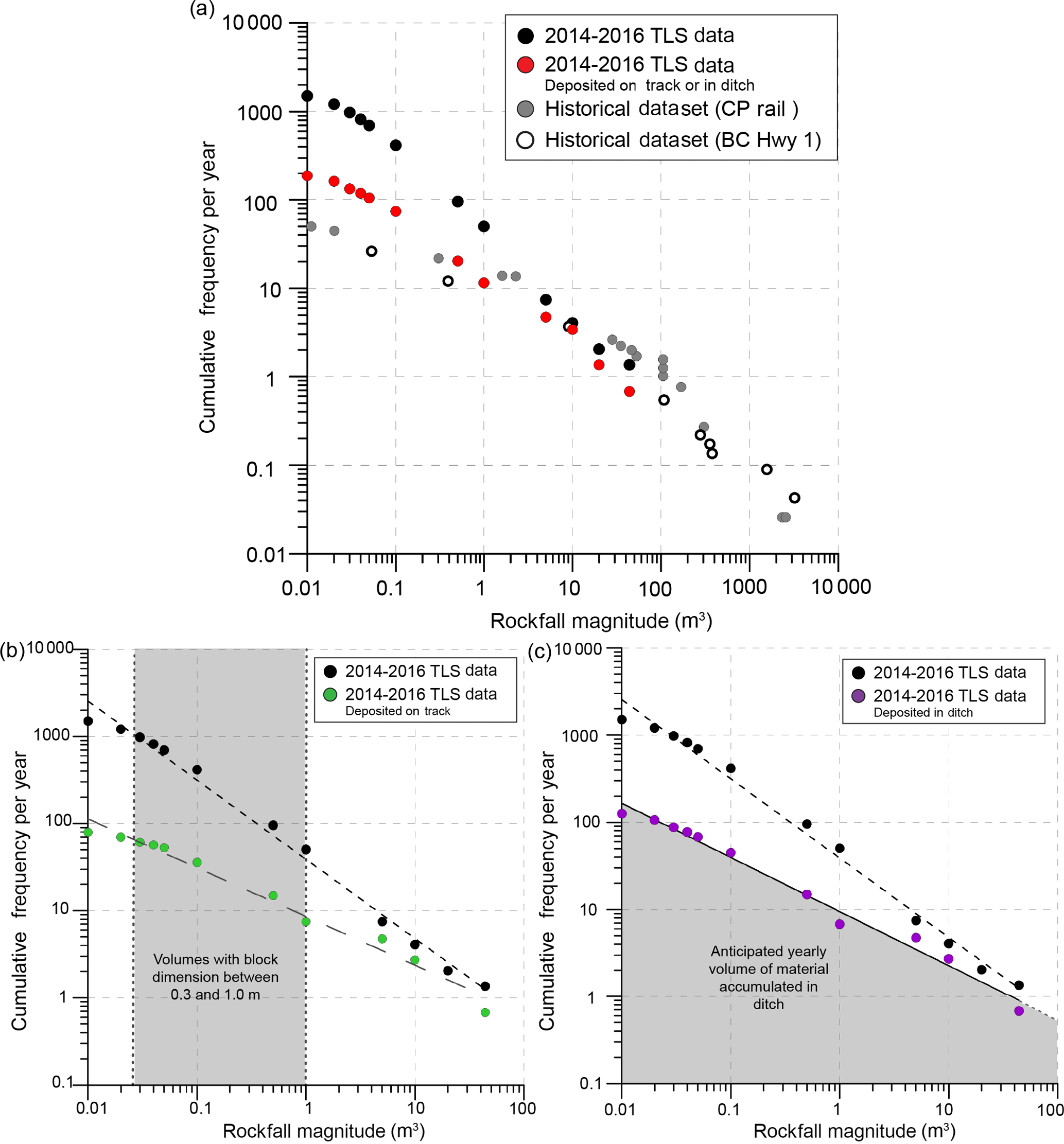
Figure 10(a) Modified MCF curves for rockfalls deposited on track or in the ditch compared to TLS inventory and historical data, (b) modified MCF curves for rockfalls deposited on track compared to TLS inventory and (c) modified MCF curves for rockfalls deposited in the ditch compared to TLS inventory.
4.1 Refinement of hazard likelihood
The results of the RockyFor3D models (deposition percentages) were applied to the database of rockfalls identified from TLS data to reproduce the rockfall MCF curves for several different scenarios (Fig. 10):
-
rockfalls landing in the ditch or on the tracks (what would typically go into an event database);
-
rockfalls landing on the tracks (blocks that present a derailment hazard); and
-
rockfalls landing in the ditch (and thus require maintenance activities in order to be cleared to provide future rockfall collection capacity).
The rockfall inventory based on TLS data was split into groups based on source zone distance from the tracks and rockfall volume. Rockfalls were assigned a volume group by rounding the volume of each event to the closest modelled volume, e.g., a rockfall with volume 0.7 m3 would be assigned to the 1 m3 volume group. Each group was randomly subsampled based on the probability of a rockfall with that source distance and volume making it to the track or ditch, and the subsampled inventory was used to develop refined MCF curves for each scenario.
In comparing the reproduced MCF curves for rockfalls deposited on tracks or in the ditch to the rockfall sources identified through TLS change detection, the yearly cumulative rockfall frequencies are up to an order of magnitude lower. The difference between the yearly frequencies becomes smaller as the rockfall magnitude increases, as these blocks have a higher probability of travelling to the base of the slope. In comparing the frequency of rockfalls deposited in the ditch or on the tracks to the frequency reported in the historical inventories, the number of events between 0.01 and 0.3 m3 that are deposited on the track or in the ditch (based on the model) is larger than reported in the historical inventories. This suggests that these inventories may contain an under sampling of small rockfall events (or that the frequency of smaller events on this individual slope is higher than the overall trend for the region). For rockfall volumes greater than 0.3 m3, the yearly frequency of events is lower than the historically recorded frequencies and could be a result of the short duration of TLS data collection (18 months).
These adjusted curves can be used to calculate the annual frequency of rockfalls deposited on the tracks that present a derailment hazard (rockfalls that land on the tracks and have a particle dimension between 0.3 and 1.0 m). Based on the curves shown in Fig. 10b, the frequency of events this size occurring on the slope is 997 rockfalls per year, but the frequency of events deposited on the track is only 56 rockfall events per year.
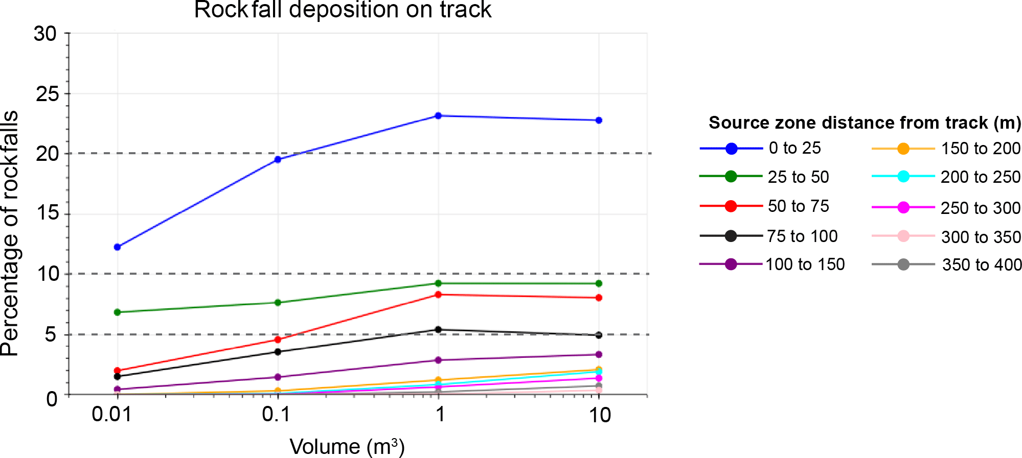
Figure 11Rockfalls deposited on track with 5 %, 10 % and 20 % exceedance criteria identified.
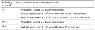
The rockfall deposition curves can be used to understand which rockfall source locations may produce rockfall events that exceed susceptibility criteria set out by rail operators. For example, based on the results presented in Fig. 11, if the railway were to accept a 10 % probability of an event landing on the tracks, given the rockfall source location and volume, then areas of concern would be any rockfall sourced from 0 to 25 m distance. This example and other scenarios are outlined in Table 3.
Table 3Locations and block sizes that exceed several conceptual probability thresholds.
4.2 Railway maintenance planning
Similar to how these adjusted curves can be used to calculate the annual frequency of rockfalls deposited on the railway tracks, they can also be used to calculate the frequency of events deposited in the ditches. Relating the frequencies of events to volume, the expected total yearly accumulation of material in the ditches can be calculated (Fig. 10c). This will provide an estimate of the maintenance work that is likely to be expected in order to retain sufficient ditch collection capacity.
We have presented a workflow for using 3-D remote sensing data to identify rockfall locations, volumes and source zone characteristics and to perform slope classifications. These data can then be used to develop rockfall simulations which can help in understanding the likelihood of these events reaching track level. Using the classified 3-D slope models, we can logically differentiate between different zones on the slope to estimate modelling parameters. The results of these models can be used to determine a more refined estimate of hazard frequency and to understand which areas of the slope may produce rockfalls that exceed susceptibility criteria set out by the rail operators. Recent studies have shown that it is possible to identify deformation of rock blocks and estimate their volume prior to failure, and this can be used to give warning to the railways of potential slope instabilities (Kromer et al., 2016). Understanding the likelihood of a block being deposited at track level based on its volume and source zone location can help to identify if a deforming block has the potential to present a hazard. It is important to note that these methods present the likelihood of a block being deposited on the tracks but do not consider blocks which may have sufficient energy to damage the tracks and cause derailment.
The MCF curve for rockfall source zones identified from TLS shows a power law fit for volumes greater than 0.02 m3; however, the curve based on rockfalls deposited in the ditch or at track level (based on probabilities from modelling) shows some rollover for volumes in the lower magnitude ranges. Many studies (Hungr et al., 1999; Dussauge-Peisser et al., 2002) have reported that the rollover in historical rockfall inventories is due to a sampling bias in the lower magnitude ranges; however, if the rockfall events occurring on the slope truly follow a power law, and smaller events are less likely to travel towards the bottom of the slope, then an inventory based only on track and ditch inspections would be expected to show rollover in the lower volume ranges regardless of any sampling bias.
Data from the White Canyon has been used as a case study to develop and present the methods described in this paper; however, these models have not been fully calibrated due to the large window between sampling periods, which may prevent us from identifying all individual rockfall events if multiple events occur in the same location during the sampling period (van Veen et al., 2017). It is also more difficult to map rockfall trajectories from the change detection results, to validate the models, when the duration between scans is increased. The overall duration of data collection has been limited to only 18 months, thus the inventory is lacking in detail for larger volume rockfalls that occur less frequently. As more data is acquired and processed, the modelling parameters can be refined, MCF curves updated and hazard frequencies adjusted.
Similar to many standard rockfall modelling software packages, the RockyFor3D model does not take into account fragmentation of rock blocks upon impact or deposition. In addition, and as is the case with many large rock slopes which are difficult to physically access, we do not have sufficient data such as physical tests or high temporal monitoring to calibrate models of rockfall fragmentation on this slope. Therefore, the deposited volumes and block sizes are likely smaller than the source zone volumes. While it is possible to determine the energy statistics at a given cell in the RockyFor3D raster model, the ability to track individual rockfall events including their passages and energies at a given location is not possible. However, this capability can help to separate events that are deposited into talus channels vs. rocks that are passing primarily over outcrop, to better understand how rockfalls behave on this complex slope. Ongoing work involves the development of a fully 3-D rockfall model using the Unity game engine (Ondercin, 2016) which will consider the influence of these factors (Sala et al., 2017). Additional work utilizing the inventory of rockfall events is focused on developing a logic for identifying rockfall source zones based on multiple factors, considering the slope geometry required to produce rockfalls of varying magnitudes. This will in turn be used to refine the rockfall simulations.
Remote sensing data can be used to collect data for hazardous rock slopes along rail corridors that may otherwise be inaccessible. Detailed geometrical data and high-resolution images derived from these methods can be used to create 3-D slope classifications and assess general structural characteristics. By performing change detection, it is possible to extract rockfall information and create an inventory of the source zones, approximate volume and timing of the events. As shown in this paper, a rockfall source zone inventory can be used in its simplest form to assess the slope angle from which rockfalls are sourced, and to provide an assessment of the magnitude–frequency relationship for the slope. The challenge remains to understand which rockfall sourced on the slope will make it to track level.
This study serves to outline a methodology and workflow that can be applied to rock slope stability and rockfall hazard assessment. Rockfall simulations can be used to determine the likelihood of a rockfall impacting the railways tracks given its volume and source zone location, which can be used to better understand the hazard likelihood and provide estimates of volumes that could accumulate in catchment ditches. The methods developed have the potential to incorporate new data as it becomes available and can be applied to additional slopes in the future.
The primary limitation of the methods described is incorporating rockfall fragmentation into the simulations, as it is difficult to calibrate fragmentation models for largely inaccessible slopes with discontinuous temporal datasets. In addition, many simulation programs do not effectively model fragmentation. As further improvements are made to simulation packages to accurately model rockfall fragmentation, the methods presented can be extended to additional software.
The underlying research data for this project can not be made publicly available as they are commercially sensitive and permission must be granted by our industry partners to access the data.
MvV coordinated the project, analyzed the data and prepared the manuscript. MvV, DJH and MO developed the framework for the study. MO and DAB developed the simulation code with input from ZS. DAB ran the simulations. ML provided technical support throughout different stages of the study. All co-authors provided manuscript review.
The authors declare that they have no conflict of interest.
This research was supported by the Canadian Railway Ground Hazards Research
Program, funded by CN Rail, Canadian Pacific and an NSERC CRD grant, and
supported by Transport Canada and the Geological Survey of Canada. Student
scholarship funding was also provided by BGC Engineering through the NSERC
IPS program. Acknowledgements are given to Emily Rowe and Ryan Kromer for
their assistance with field data collection and to the Kumsheen Rafting
Resort and CN Rail for providing site access and logistical support.
Edited by: Thomas Glade
Reviewed by: Olga Mavrouli and one anonymous referee
Abbott, B., Bruce, I., Keegan, T., Oboni, F., and Savigny, W.: Application of a New Methodooogy for the Management of Rockfall Risk Along a Railway, 8th International Association of Engineering Geology Conference, A Global View from the Pacific Rim, Vancouver, 1998a.
Abbott, B., Bruce, I., Savigny, W., Keegan, T., and Oboni, F.: A Methodology for the Assessment of Rockfall Hazard Risk along Linear Transportation Corridors, 8th International Association of Engineering Geology Conference, A Global View from the Pacific Rim, Vancouver, BC, 1998b.
Agisoft: Agisoft Photoscan Professional Edition, v. 1.2.3, Agisoft LLC, St. Petersburg, Russia, 2015.
Besl, P. J. and McKay, N. D.: A Method for the Registration of 3-D Shapes, IEEE T. Pattern Anal., 14, 239–256, 1992.
Bonneau, D. and Hutchinson, D. J.: Applications of Remote Sensing for Characterizing Debris Channel Processes, Landslides: Putting Knowledge, Experience and Emerging Technologies in to Practice, AEG Special Publication No. 27, 2017.
Brown, D. A.: Geology of the Lytton Area, British Columbia, BSc Honours, Carleton University, Ottawa, Canada, 1981.
Corominas, J., Matas, G., and Ruiz-Carulla, R. The Fragmentation of Rockfall and the Analysis of Risk, Geohazards 7, Canmore, Alberta, 2018.
D'Amato, J., Guerin, A., Hantz, D., Rossetti, J. P., and Jaboyedoff, M.: Terrestrial Laser Scanner study of rockfall frequency and failure configurations, Troisièmes Journées Aléas Gravitaires, Grenoble, France, 2013.
Deere, D. U. and Miller, R. P.: Engineering Classification and Index Properties of Intact Rock, Air Force Weapons Laboratory, Kirkland Air Force, New Mexico, 1966.
Dorren, L. K. A.: Rockyfor3D(v5.2) revealed – Transparent description of the complete 3D rockfall model, ecorisQ paper, 32, 1–32, 2015.
Dussauge-Peisser, C., Helmstetter, A., Grasso, J.-R., Hantz, D., Desvarreux, P., Jeannin, M., and Giraud, A.: Probabilistic approach to rock fall hazard assessment: potential of historical data analysis, Nat. Hazards Earth Syst. Sci., 2, 15–26, https://doi.org/10.5194/nhess-2-15-2002, 2002.
Guerin, A., Hantz, D., Rossetti, J.-P., and Jaboyedoff, M.: Brief communication “Estimating rockfall frequency in a mountain limestone cliff using terrestrial laser scanner”, Nat. Hazards Earth Syst. Sci. Discuss., 2, 123–135, https://doi.org/10.5194/nhessd-2-123-2014, 2014.
Hungr, O., Evans, S. G., and Hazzard, J.: Magnitude and frequency of rock falls and rock slides along the main transportation corridors of southwestern British Columbia, Canadian Geotechnical Journal, 36, 224–238, 1999.
Hutchinson, D. J., Lato, M., Gauthier, D., Kromer, R., Ondercin, M., van Veen, M., and Harrap, R.: Applications of remote sensing techniques to managing rock slope instability risk, Canadian Geotechnical Conference, Quebec City, 20–23 September 2015.
Jolivet, D., MacGowan, T., McFadden, R., and Steel, M.: Slope Hazard Assessment using Remote Sensing in White Canyon, Lytton, BC, Report submitted to the Department of Geological Science and Geological Engineering, Queen's University, Kingston, ON, Canada, 2015.
Kromer, R., Hutchinson, D. J., Lato, M., Gauthier, D., and Edwards, T.: Identifying rock slope failure precursors using LiDAR for transportation corridor hazard management, Eng. Geol., 195, 93–103, https://doi.org/10.1016/j.enggeo.2015.05.012, 2015.
Kromer, R., Hutchinson, D. J., Lato, M., and Abellán, A.: Rock Slope Pre-failure Deformation Database for Improved Transportation Corridor Risk Management, International Symposium on Landslides, Naples, Italy, 2016.
Lan, H., Martin, C. D., Zhou, C., and Lim, C. H.: Rockfall hazard analysis using LiDAR and spatial modeling, Geomorphology, 118, 213–223, https://doi.org/10.1016/j.geomorph.2010.01.002, 2010.
Marinos, P. and Hoek, E.: GSI: A Geologically Friendly Took for Rock Mass Strength Estimation, Proceedings of GeoEng2000, Melbourne, 2000.
Ondercin, M.: An Exploration of Rockfall Modelling Through Game Engines, MASc, Geological Sciences and Geological Engineering, Queen's University, Kingston, Canada, 2016.
Ondercin, M., Kromer, R., and Hutchinson, D. J.: A comparison of rockfall models calibrated using rockfall trajectories inferred from LiDAR change detection and inspection of gigapixel photographs, 6th Canadian Geohazards Conference, Kingston, Ontario, Canada, 2014.
Rosser, N. J., Petley, D. N., Lim, M., Dunning, S. A., and Allison, R. J.: Terrestrial laser scanning for monitoring the process of hard rock coastal cliff erosion, Q. J. Eng. Geol. Hydroge., 38, 363–375, https://doi.org/10.1144/1470-9236/05-008, 2005.
Rowe, E., Hutchinson, D. J., and Kromer, R.: An Analysis of Failure Mechanism Constraints on Pre-Failure Rock Block Deformation using TLS and Roto-Translation Methods, Landslides, 15, 409–421, https://doi.org/10.1007/s10346-017-0886-8, 2018.
Sala, Z., Hutchinson, D. J., and Ondercin, M.: Application of the Unity Rockfall Model to Variable Surface Material Conditions, 2017 EGU General Assembly, Vienna, Austria, 2017.
Santana, D., Corominas, J., Mavrouli, O., and Garcia-Sellés, D.: Magnitude–frequency relation for rockfall scars using a Terrestrial Laser Scanner, Eng. Geol., 145–146, 50–64, https://doi.org/10.1016/j.enggeo.2012.07.001, 2012.
van Veen, M., Hutchinson, D. J., Gauthier, D., Lato, M., and Edwards, T.: Classification of Rockfall Patterns Using Remote Sensing Data For Hazard Management in Canadian Rail Corridors, 2016 Canadian Geotechnical Conference, Vancouver, British Columbia, Canada, 2016.
van Veen, M., Hutchinson, D. J., Kromer, R., Lato, M., and Edwards, T.: Effects of sampling interval on the freqeucny-magnitude relationship of rockfalls detected from terrestrial laser scanning using semi-automated methods, Landslides, 14, 1579–1592, https://doi.org/10.1007/s10346-017-0801-3, 2017.