the Creative Commons Attribution 4.0 License.
the Creative Commons Attribution 4.0 License.
 | 04 Sep 2018
Evaluation of predictive models for post-fire debris flow occurrence in the western United States
Efthymios I. Nikolopoulos
Elisa Destro
Md Abul Ehsan Bhuiyan
Marco Borga
Emmanouil N. Anagnostou
Rainfall-induced debris flows in recently burned mountainous areas cause significant economic losses and human casualties. Currently, prediction of post-fire debris flows is widely based on the use of power-law thresholds and logistic regression models. While these procedures have served with certain success in existing operational warning systems, in this study we investigate the potential to improve the efficiency of current predictive models with machine-learning approaches. Specifically, the performance of a predictive model based on the random forest algorithm is compared with current techniques for the prediction of post-fire debris flow occurrence in the western United States. The analysis is based on a database of post-fire debris flows recently published by the United States Geological Survey. Results show that predictive models based on random forest exhibit systematic and considerably improved performance with respect to the other models examined. In addition, the random-forest-based models demonstrated improvement in performance with increasing training sample size, indicating a clear advantage regarding their ability to successfully assimilate new information. Complexity, in terms of variables required for developing the predictive models, is deemed important but the choice of model used is shown to have a greater impact on the overall performance.


Wildfires constitute a natural hazard with devastating consequences to the natural and built environment. In addition to the immediate impact of wildfire events to human lives, infrastructure and the environment, their adverse effects on landscape characteristics generate a cascade of hydrogeomorphic hazards (Shakesby and Doerr, 2006; Parise and Cannon, 2012; Diakakis et al., 2017). One of the most frequent post-fire hazards is debris flow. Debris flows are rapidly flowing, gravity-driven mixtures of sediment and water, commonly including gravel and boulders (Iverson, 2005), which rush down on steep channels and discharge onto debris fans, posing a significant threat to downstream populations.
Post-fire debris flows (hereinafter DF) are predominantly derived from channel erosion and incision, usually generated during heavy precipitation events on burned areas (Cannon and DeGraff, 2009; Parise and Cannon, 2017). Recent studies have shown that in fire-affected regions the threat associated with debris flows may persist for several years after the fire incident (DeGraff et al., 2013; Diakakis et al., 2017), demonstrating the necessity for developing short and long-term plans for the mitigation of this hazard (DeGraff et al., 2013).
In the western United States, DF is a well-recognized hazard that has claimed human lives and caused severe damage to infrastructure over the years (Cannon et al., 2003; Coe et al., 2003; Cannon and Gartner, 2005; Santi et al., 2008). The occurrence of the DF hazard in this region is expected to further intensify due to an expected increase in fire occurrence and fire season length, as a result of climate change (Riley and Loehman, 2016), and the continuous population growth on the wildland–urban interface (Cannon and DeGraff, 2009). Therefore, developing effective measures to reduce the vulnerability of local communities to DF is of paramount importance.
Early warning is a critical element for the successful mitigation of DF hazard. Over the last decade a number of researchers have worked on developing procedures for predicting DF in the western United States (Cannon et al., 2008; DeGraff et al., 2013; Staley et al., 2013). In addition, federal agencies associated with monitoring and forecasting natural hazards like the United States Geological Survey (USGS), National Oceanic and Atmospheric Administration (NOAA) and National Weather Service (NWS) have jointly developed a debris flow warning system for recently burned areas (Restrepo et al., 2008). In their vast majority, the foundations of these warning procedures lie on empirical relationships that are used to identify the conditions likely to lead to the occurrence of DF. In their simplest form, these relationships refer to rainfall intensity (or accumulation–)duration thresholds above which DF is likely to occur (Cannon et al., 2008; Staley et al., 2013). Other procedures involve the application of statistical models that incorporate information on land surface characteristics (e.g., percentage of burned area, local topographic gradients), in addition to rainfall properties, to predict the likelihood of a DF occurrence. The most commonly used statistical model for DF prediction is the logistic regression model (Rupert et al., 2008; Cannon et al., 2010). Updates of these past prediction models were recently suggested by Staley et al. (2017), who proposed a new logistic regression model that improves current DF prediction procedures in the western United States. Additionally, in a recent study by Kern et al. (2017), a number of machine-learning approaches were evaluated for DF prediction. The conclusions based on that study is that advanced statistical modeling techniques can offer significant improvement in the performance of current DF prediction models.
Both of the recent works of Staley et al. (2017) and Kern et al. (2017) suggest that, although models for DF prediction may already exist for specific regions (Cannon et al., 2010), the importance of improving their accuracy and also extending prediction beyond the boundaries of these regions calls for continuous advancements of currently established procedures. Following this line of thought, this study focuses on the development of a new DF prediction model that is based on a nonparametric statistical approach and the evaluation of its performance against state-of-art approaches for DF prediction in the western United States. Specifically, we evaluate the performance of four models that include (i) rainfall accumulation–duration thresholds (Guzzetti et al., 2007; Cannon et al., 2011; Rossi et al., 2017; Melillo et al., 2018), (ii) the logistic regression model suggested by Staley et al. (2017) and (iii) two models based on the random forest technique (Breiman, 2001) that are introduced in this study. In addition to the consistent evaluation of the performance of each model, this work investigates the relationship between prediction accuracy with complexity and data requirements (in terms of both record length and variables required) of each model. These are important aspects for selecting the most appropriate method and for providing guidance for data scarce regions on global scale.

Figure 1Location of all post-fire debris flow records included in the USGS database. Note that all events in Utah and Montana were excluded from the analysis due to their incomplete record of variables.
Table 1A summary of variables reported in the post-fire debris flow database.
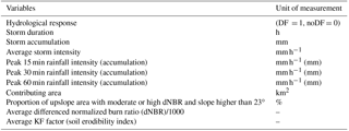
This study is based on a USGS database that was recently published (Staley et al., 2016) and includes information on the hydrologic response of several burned areas in the western United States (Fig. 1). The database reports the occurrence of debris flow (DF) or no-debris flow (noDF), and rainfall characteristics for 1550 rainfall events in the period 2000–2012 together with field-verified information characterizing the areas affected by wildfires (Table 1). The area of fire-affected catchments analyzed varied between 0.02 and 7.9 km2. Rainfall data were collected from rain gauges located within a maximum distance of 4 km from the documented response location. Reported rainfall characteristics included rainfall peak intensities (and accumulations) at 15, 30 and 60 min time intervals, event total accumulation, duration and average intensity. According to the description of the data set provided in Staley et al. (2016), the rainfall characteristics (peak intensities, accumulation, etc.) were calculated using a backwards differencing approach (Kean et al., 2011). Land surface characteristics of burned areas were recorded in order to evaluate the influence of the burned area to the hydrologic response. Information on burn severity was based on the differenced normalized burn ratio (dNBR) (Key and Benson, 2006), calculated from near-infrared and shortwave-infrared observations, which is frequently used for the classification of burn severity (Miller and Thode, 2007; Keeley, 2009). Severity classification from dNBR was validated from field observations provided by local burned area emergency response teams. In addition to dNBR, the database includes information on the proportion of the upslope catchment area that has been classified at high or moderate severity and with terrain slope higher than 23∘. Finally, since in burned areas changes in recovery vegetation increase erosion, the average erodibility index (KF factor) derived from the STATSGO database (Schwartz and Alexander, 1995) is reported in the database as well. The KF factor provides evidence of erodibility of soil, taking into account the fine-earth fraction (< 2 mm). For more information on the estimation procedures of the variables (Table 1), the interested reader is referred to Staley et al. (2016) and references therein.
The 334 events (∼22 %) of hydrologic responses in the database were identified as debris flows. The location of events in the data set corresponds predominantly to the area of southern California (CA), which includes 61 % (60 %) of all records (DF records). Colorado (CO) corresponds to 20 % (10 %) of the data (DF) and the rest of the data correspond to other regions – Arizona (AZ), New Mexico (NM), Utah (UT) and Montana (MT) – of the western United States (Fig. 1). Since values for some of the variables (e.g., rainfall duration, 15 min peak intensity) are not reported consistently for all records, the analysis presented hereinafter is focused only on the 1091 events with a complete record that involve the areas of Arizona, California, Colorado and New Mexico.
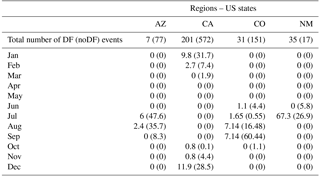
Table 2Total number and monthly distribution of DF and noDF events analyzed for Arizona, California, Colorado and New Mexico. Values per month correspond to percentage (%) of the total number of events (DF + noDF) analyzed per region.
Most of the western United States is characterized by dry summers, when the fire activity is widespread, with a high percentage (50 %–80 %) of annual precipitation falling during October–March. However, there are also regions, such as Arizona and New Mexico, where heavy rains occur between July and August as a result of the North American monsoon (Westerling et al., 2006). More specifically, four different seasonal rainfall types characterize the southwestern United States (Moody and Martin, 2009): Arizona, Pacific, sub-Pacific and plains types. Arizona is characterized by dry spring, moist fall and wet winter and summer; California is mainly characterized by Pacific-type rainfall, with a maximum in winter and extremely dry summer. The sub-Pacific type, with a wet winter, moist spring and summer, and dry fall, characterizes the southern part of the Sierra Nevada region, a small area in southern California. A climate similar to Arizona type characterizes southwestern Colorado, while east Colorado is characterized by plains, where the rainfall maxima occur in summer. The Arizona type also characterizes western New Mexico, while the eastern part is characterized as plains.
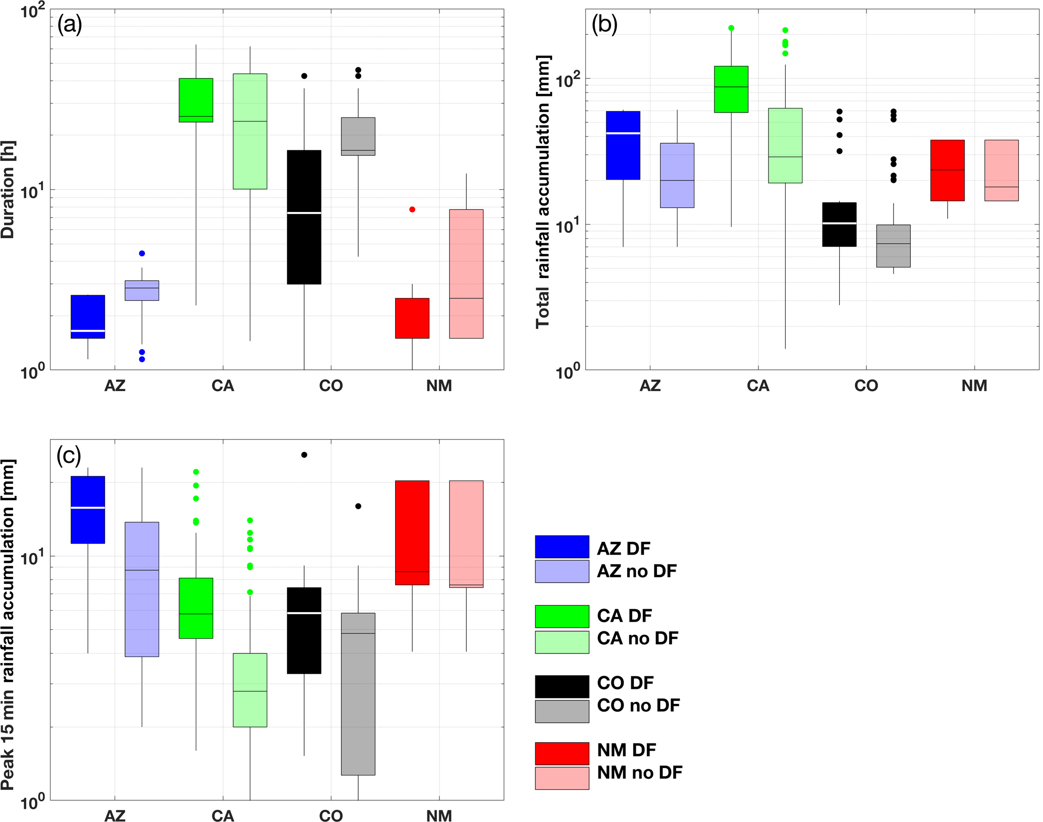
Figure 2Box plot for (a) storm duration, (b) storm accumulation and (c) peak 15 min storm accumulation for Arizona (blue), California (green), Colorado (black) and New Mexico (red). Dark (light) colors correspond to DF and noDF events.
Examination of the seasonality of the rainfall events analyzed (Table 2) demonstrates the similarities and differences attributed to the different climate types described above. The vast majority (92 %) of rainfall events in Arizona occurred during the summer months (July and August). Similarly, the majority of rainfall events in western Colorado occurred during late summer–early fall months (August and September). California, which is influenced by the Pacific rainfall regime, is dominated by winter rainfall events, where 82 % of events occurred between December and January. Seasonality of rainfall events for New Mexico exhibits a characteristic dominance of occurrences in summer, with 94 % of the events occurring in July and the remainder in June.
The North America monsoon is responsible for the summer rainstorms in these regions that typically last between June and mid-September, causing strong thunderstorm activities in the uplands of Arizona and New Mexico and the absence of rainy events in southern California (Mock, 1996; Adams and Comrie, 1997). September is the rainiest month in Colorado because of midlatitude cyclones coming from the Gulf of Alaska (Mock, 1996).
Differences in seasonality and large-scale climatic controls essentially correspond to differences in dominant precipitation type (e.g., convective vs. stratiform) and differences in characteristic properties of rainfall events triggering debris flows (Nikolopoulos et al., 2015). Analysis of the characteristics of the rainfall events revealed clear regional dependences and for certain regions there were also distinct differences in the characteristics between DF and noDF events (Fig. 2).
Rainfall duration for events in Arizona and New Mexico is significantly lower than events in other regions, with California being associated with the longest events (10–70 h in most cases), typical for the winter-type rainfall that is dominant in this region. The DF-triggering events for Arizona, Colorado and New Mexico correspond to the shortest events, while the opposite is shown for California (Fig. 2a). Variability among regions and within noDF and DF-triggering events also exists for the magnitude of rainfall events (Fig. 2b, c). With the exception of events in New Mexico, the other regions exhibit a distinct separation in the distribution of total rainfall accumulation (Fig. 2b) and peak 15 min accumulation (Fig. 2c) between DF and noDF events. For these regions, the highest values for both variables are associated with the DF-triggering events, which justifies the rational for using these variables for predicting DF occurrence.
In addition to the marginal distribution of the rainfall variables shown in Fig. 2, the relationship between duration and magnitude is presented in Fig. 3. California events are distinctly clustered over the high accumulation–duration area (Fig. 3a), demonstrating the discussed regional dependence of rainfall characteristics. The total rainfall accumulation is strongly correlated with duration for the DF-triggering events (Pearson's correlation coefficient 0.7). On the other hand, the peak 15 min accumulation, which is a proxy for the maximum intensity of the events, does not correlate well with duration (Pearson's correlation coefficient −0.2). Overall, it is apparent from Fig. 3 that there are areas in the accumulation–duration spectrum where the DF and noDF events are well mixed, which highlights the challenge of identification between the two and the need for classification approaches based on additional parameters.
Findings from the analysis of rainfall seasonality provide clear indications that there are distinct regional differences in the triggering rainfall characteristics. This justifies the development of regional predictive models as stated in past studies and raises an important point of consideration for creating a single multi-region-wide framework for DF prediction. The issue of regional dependence and how it can be incorporated into a single model is further discussed in Sect. 4.1.3 below.
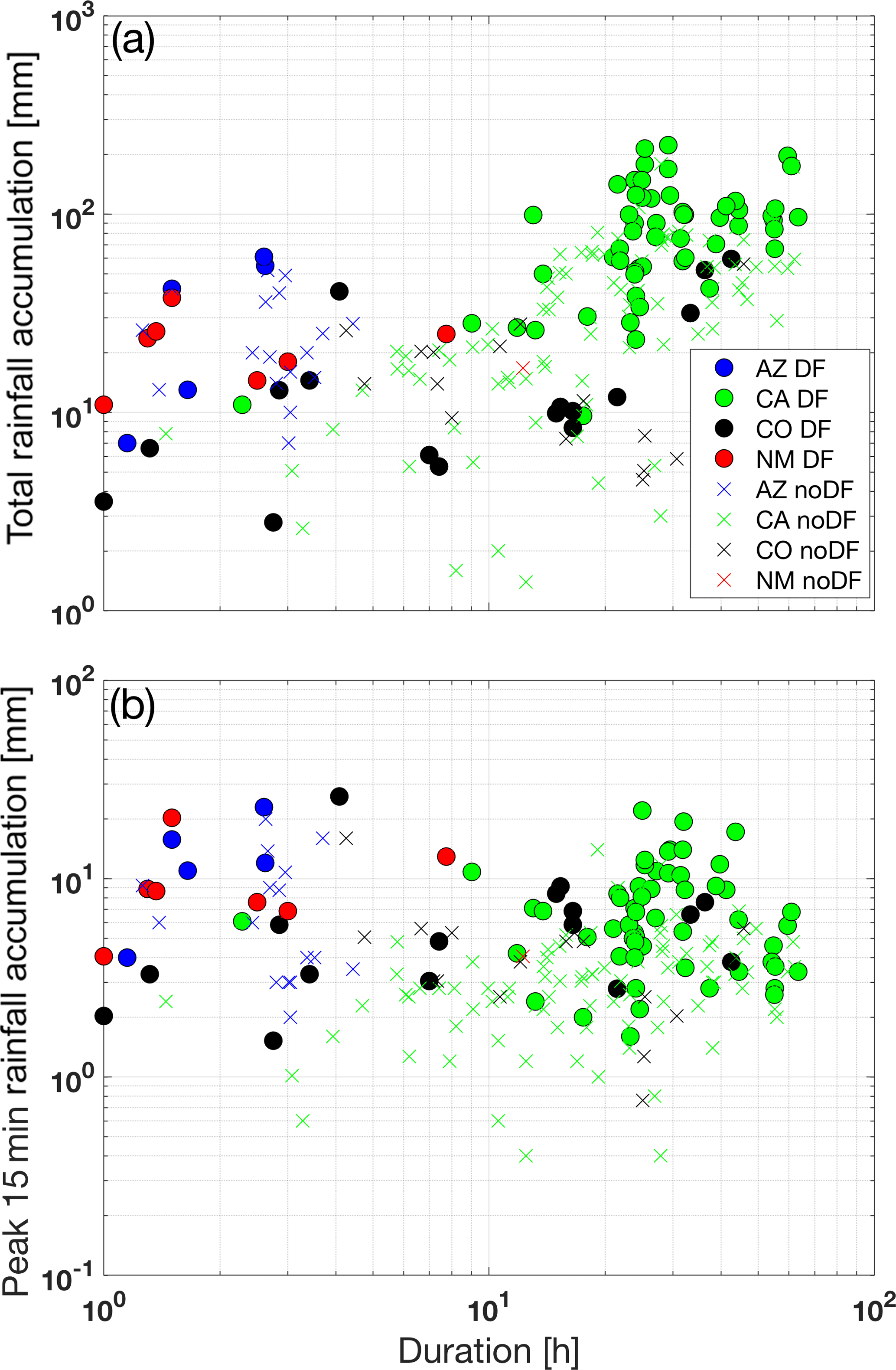
Figure 3(a) Total rainfall accumulation vs. duration and (b) peak 15 min rainfall accumulation vs. duration for Arizona, California, Colorado and New Mexico. Colored dots and x symbols correspond to DF and noDF occurrences, respectively.
4.1 Models for predicting post-fire debris flow occurrence
This section describes the different models that will be evaluated for predicting the occurrence of post-fire debris flow (PFDF). Selection of the different models is based on criteria of model simplicity, data requirements and relevance to common practice.
4.1.1 Rainfall thresholds
Rainfall thresholds correspond to one of the simplest and most widely used approaches for predicting the occurrence of rainfall-induced mass movements such as shallow landslides and debris flows (Caine, 1980, Guzzetti et al., 2007, Cannon et al., 2011). Rainfall thresholds are commonly formulated as power-law relationships that link rainfall magnitude and duration characteristics, as in the following:
where total event rainfall accumulation (E) is related to event duration (D). The intercept (α) and exponent (β) are parameters estimated from the available observations. In this case, the threshold (hereinafter ED threshold) provides the rainfall accumulation, above which a debris flow event will occur for a given duration. In this work, the parameter β was estimated according to the slope of log(E) vs. log(D) using least squares linear regression and considering only the events that resulted in debris flows. The full record (both DF and noDF events) was then used to identify the optimum value of parameter α. Details on the optimization of parameter α and the criteria used are discussed in Sect. 4.3.
4.1.2 Logistic regression
Another model that is frequently used for modeling the statistical likelihood of a binary response variable is the logistic regression (LR) model. In the western United States, LR models were first developed for DF prediction almost a decade ago (Rupert et al., 2008; Cannon et al., 2010) and are still used to date (Staley et al., 2016, 2017).
The probability of occurrence (P) of PFDF according to logistic regression is given as
where the link function x is modeled as a linear combination of one or more explanatory variables according to
where Xn is the nth explanatory variable and γ and
δn are parameters estimated from the observation data set.
Selection of the explanatory variables is very crucial for successfully
developing LR models. In this study, we adopted the latest LR model proposed
by Staley et al. (2016, 2017), which can also be considered to be the
state of the art for DF prediction in the western United States. After a thorough
examination of several LR models, the authors of those works concluded that
the most appropriate set of explanatory variables are
X1= max 15 min rainfall accumulation × proportion of upslope area
burned at high or moderate severity with gradients ;
X2= max 15 min rainfall accumulation × average dNBR normalized by
1000;
X3= max 15 min rainfall accumulation × soil KF factor.
Based on this formulation, information on the maximum 15 min rainfall
accumulation is used to weigh the other three parameters (upslope burned
area, average dNBR and KF factor). Parameters γ and
δn were estimated based on least squares regression.
Specifically, the glmfit function of MATLAB software (version 2017b) was
used to fit the binomial distribution to available data using the logit link
function.
4.1.3 Random forest
Random forest (RF) is a nonparametric statistical technique that is based on the decision tree ensemble (i.e., forest) procedure for classification or regression (Breiman, 2001). Despite being a well-known algorithm with extensive use in other fields (e.g., medicine), there are not many examples of RF applications in hydrogeomorphic response studies and most of them deal with landslide susceptibility (e.g., Brenning, 2005; Vorpahl et al., 2012; Catani et al., 2013; Trigila, 2015). Some of the main advantages of RF algorithm are that it allows numerical and categorical variables to be mixed and it does not require any knowledge on the distribution of variables and the relationship between them. In this work, we used RStudio software and the R package randomForest (Liaw and Wiener, 2002) to develop the RF model for PFDF prediction.
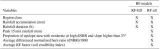
For the selection of the most important variables for the RF model we tested several different scenarios of variable combinations. During that investigation, we found that the use of an extra categorical variable (named “region class” hereinafter) that is used to classify the data set into two geographic regions (i.e., within California and other) improves RF model performance and thus was included in the variables used for the RF development. Explanation for the importance of this regional distinction lies on the existence of a clear difference in the seasonality and subsequently rainfall characteristics between California and the other regions considered. From all the different combinations of variables tested, we identified two different models that we present and discuss in the work. The first model (RF-ED) was developed using the variables of rainfall accumulation, duration and region class. We consider it to be the one with minimum data requirements, given that only two rainfall variables and a region classification are used for the prediction. The second model (RF-all) is considered to be the data-demanding RF model and uses almost all available information on rainfall characteristics, burn severity, land surface properties, etc. Table 3 reports all the variables used in each model.
Table 3Description of variables included in the development of RF models. Symbol X denotes the variables that were included in each model.
4.2 Model performance criteria
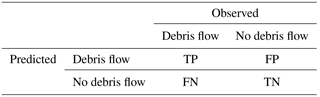
Evaluation of model performance in predicting DF occurrence was based on the contingency table (Table 4), which is used to measure the number of correct and false predictions. True positive (TP) corresponds to the number of debris flow events correctly predicted by the model, false positive (FP) indicates the number of falsely predicted debris flows, false negative (FN) is the number of missed debris flow events and true negative (TN) corresponds to the “no debris flow” events correctly predicted. The metrics, according to the contingency table, that we use in the evaluation of the predictive skill of the models are the threat score (TS), the true positive rate (TPR) and the false positive rate (FPR) defined as
The threat score (also known as the critical success index) provides information on the overall skill in predicting positive (i.e., DF) responses with respect to total (TP + FP) and missed (FN) positive predictions. TPR and FPR provide information on correct positive and false positive predictions as percentages of the total positive and negative events, respectively. Lastly, the predictive performance of the different models examined is assessed based on the receiver operating characteristic (ROC) curves (Fawcett, 2006).
4.3 Identification of thresholds
Whether using ED, LR or RF models, identification of debris flow occurrence is based on the use of a threshold value, above which we consider that a debris flow will occur. In the case of ED thresholds, the slope (parameter β) is estimated from the data (as discussed in Sect. 4.1.1) and the intercept (parameter α) is identified according to the maximization of TS. In other words, given the estimated parameter β, the ED threshold is always defined in order to achieve a maximum TS value for the data set used to train the model (see example demonstrated in Fig. 4a).
LR and RF models estimate a probability of DF occurrence for both DF and noDF events. Equivalently, this requires the selection of the appropriate threshold of the probability value above which we consider DF occurrence. Often, the probability threshold corresponds to a value of 0.5 (see for example Staley et al., 2017) but this does not necessarily imply optimum performance considering that DF and noDF events are not perfectly separated and some overlap in probability space exists (see example in Fig. 4b). During the training of both the LR and RF models, we allow the probability threshold value to be defined according, again, to the maximization of TS value.
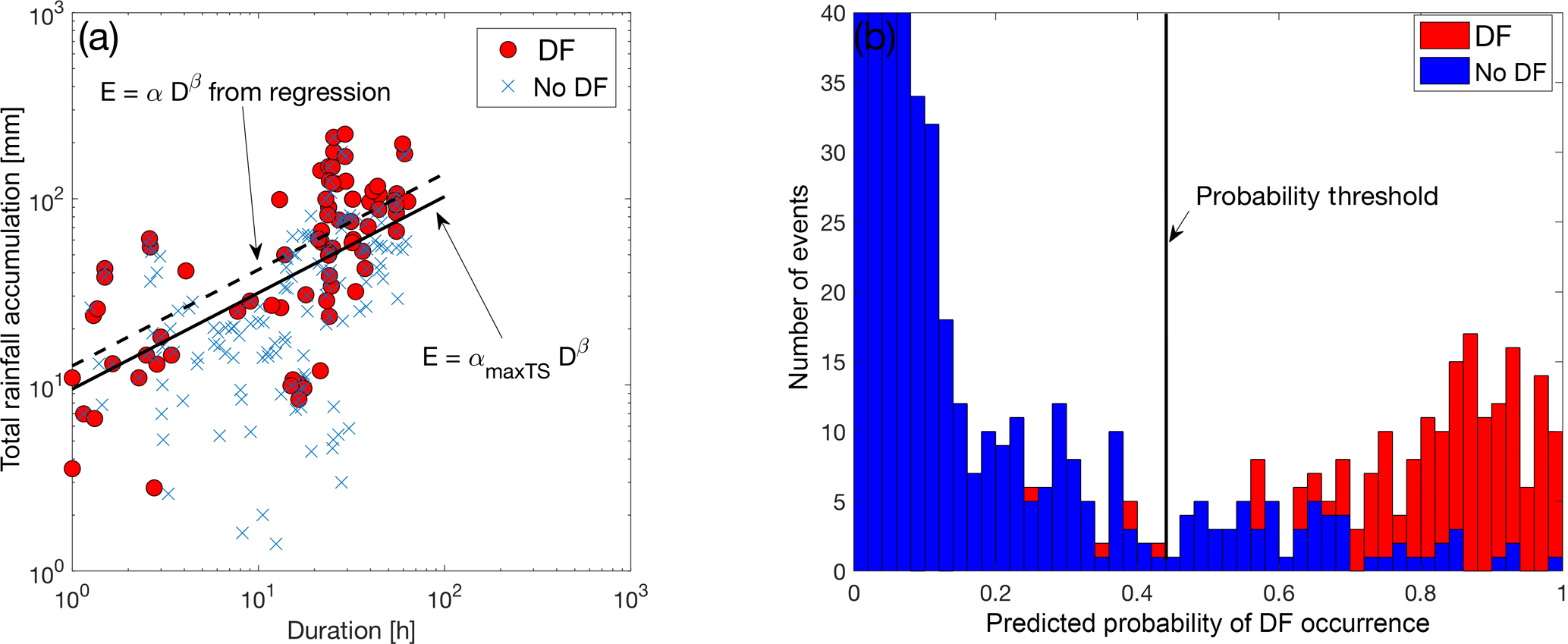
Figure 4Example plot demonstrating the (a) ED threshold and (b) probability threshold for optimizing (i.e., maximizing TS) DF prediction. In (a), the αmaxTS corresponds to the optimum intercept parameter (see Sect. 4.1.1) and in (b) the vertical black line identifies the probability value used to optimize classification between DF and noDF events.
4.4 Model training and validation framework
For training and validation of the predictive models we followed two different approaches that included a Monte Carlo random sampling and hold-one-out validation framework.
In the random-sampling framework, a training data set of size M and a test data set of size K is sampled randomly from the original data sample. The training data are used to train each model (i.e., estimate parameters for ED and LR and build RF) and then the trained models are evaluated using the test data. This random-sampling training–validation procedure was repeated 500 times to provide an estimate of the effect of sampling uncertainty on the model performance. The only condition that was imposed during the construction of the random training and test samples was the proportion of DF/noDF events in each sample. We set the percentage of DF events to be 20 % in both train and test, following approximately the same percentage used in the training data set of Staley et al. (2017), which also roughly corresponds to the percentage of DF events in the original sample as well. The test sample size K was fixed to 100, while the train sample size M was allowed to vary from 100 up to 900 to also allow investigation of the sensitivity of results to different train sample sizes.

Figure 5Sensitivity to sample size: box plots of the threat score (TS), according to the random-sampling validation framework, for increasing sample size and for the four models considered for post-fire debris flow prediction.
In the hold-one-out validation, all events in the database except one are used each time as the training data set and the models are evaluated for each event that is left out. This procedure is repeated by sequentially holding out all events, essentially allowing the models to be validated against all available events. This process somewhat mimics better what would have been done in practice, considering that in an operational-like environment we would be training our predictive models with all available historic events and use them to predict the next new event. Therefore, in this case the training sample size was equal to 1090 and was constructed by sequentially leaving one event out from the original sample size. The training–validation process was repeated until all events were included as validation points (i.e., 1091 times).
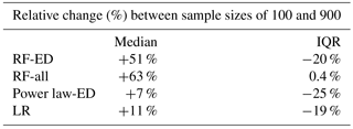
Table 5Relative change (%) in TS distribution between sample sizes of 900 and 100.
In this section, we present and discuss the findings based on the evaluation results for the different predictive models and the two validation frameworks considered.
5.1 Random-sampling validation
The random-sampling validation results (Fig. 5) demonstrate the relative performance of the models examined as a function of the training sample size. Interestingly, even for the smallest sample size examined (M=100), the RF-based models exhibit higher median values than the ED and LR models but at the same time are characterized by greater variability in their performance, manifested on the graph as larger boxes. As sample size increases, the model performance (in terms of TS values) increases for both RF-based models. An interesting point to note from these results is that for the smaller sample sizes examined (M=100–500) the RF-ED performed marginally better than the RF-all but as the sample size increased, the situation is reversed and higher TS values are associated with the RF-all model. This suggests that the increasing amount of data used for training improves the RF-based model that involves a greater number of explanatory variables at a higher rate.
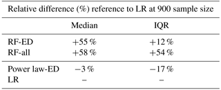
Table 6Relative difference in TS distribution between the reference model (LR) and the RF-ED, RF-all and ED models at the maximum sample size examined. Positive values denote an increase in other models relative to LR.
On the other hand, both ED and LR models exhibit consistently worse performances overall than RF-based models and a lower sensitivity to sample size.
A summary of the change in TS distribution with sample size is presented in Table 5, where the relative difference in median and interquartile range (IQR), between maximum (M=900) and minimum (M=100) sample size examined, is reported for each model. The performance of RF-ED model improved significantly with an increase in the median value of 51 % and a decrease in the IQR of 20 %. The RF-all model showed an even higher increase in the median (63 %) but variability in performance remained practically unchanged. On the other hand, the ED and LR models showed much smaller (than RF-based) median increases (7 % and 11 %) but exhibited considerable decreases in IQR (25 % and 19 %).
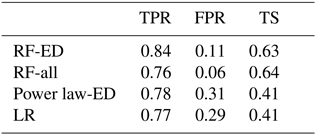
Table 7Model performance according to the thresholds based on maximization of TS.
Furthermore, the relative difference between the models is presented for the highest sample size (M=900) and with reference to the LR model, which corresponds to the current state of the art in PFDF occurrence prediction for the western United States (Staley at al., 2017). Based on the results (Table 6), the RF-ED model TS is 55 % higher than the LR model but with an increased IQR (+12 %). The RF-all model TS is 58 % higher but with significantly increased variability in performance (IQR +54 %). The ED model performs slightly worse (−3 % in median) but with reduced variability (IQR −17 %) relative to the LR model.
The results from this random-sampling validation exercise demonstrate a superior performance of the RF-based models particularly for the largest sample sizes examined. For the smallest sample size, the RF-based models are characterized by significant variability in their performance, which may raise questions regarding their applicability when short data records are available. However, for higher sample sizes and despite the fact that variability remains, the median performance increases to the degree that makes clear the distinction in performance with respect to other models. Additionally, an important note is that overall the variability of the performance of all models, for a given sample size, is considerable and this essentially highlights the effect of the sampling uncertainty; an aspect that requires careful consideration for the development and application of such predictive models.
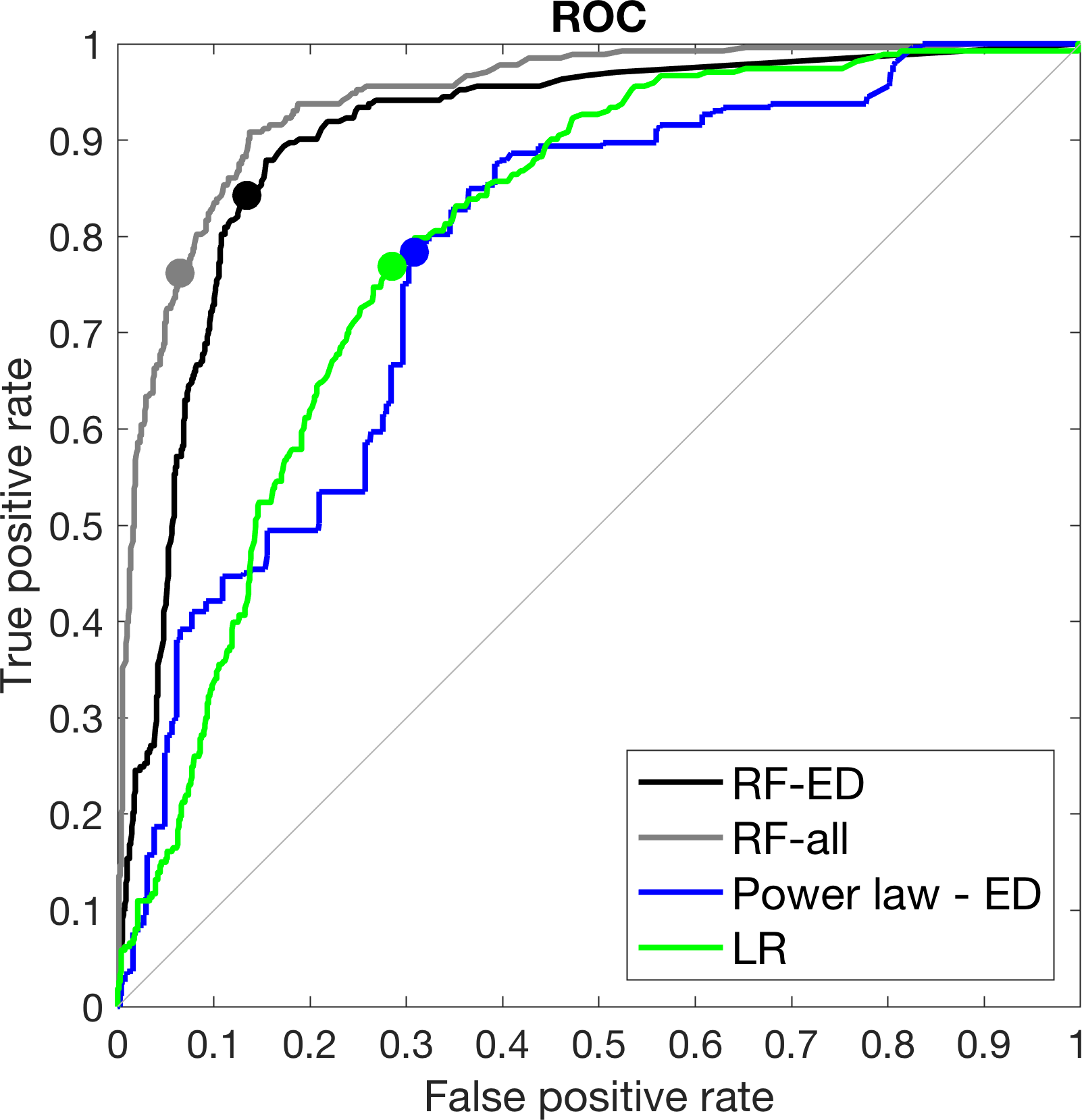
Figure 6ROC curves for the hold-one-out validation technique for the four models. Circles correspond to the model performance when selected thresholds were based on TS maximization.
5.2 Hold-one-out validation
For the hold-one-out validation, results are reported by collectively considering the model prediction outcome for all events, meaning that the prediction of all 1091 events were used to summarize the performance indicators (TS, TPR, FPR) reported in Table 7. Recall that, for the prediction of each event, each model was trained with the remaining data set (i.e., 1090 events) and thresholds were determined according to the maximization of TS in each case. According to the TS values reported, the RF-based models with TS equal to 0.63 (RF-ED) and 0.64 (RF-all) exhibit considerably improved performance with respect to the ED and LR models with TS values of 0.41 for both models. Comparison of the TPR and FPR values suggests that the superiority of RF-based models is primarily attributed to the lower false alarm rates (≤11 %) relative to ED and LR models (∼30 %). The true positive rate appears equivalent among the different models.
However, an important note here is that these metrics (TS, TPR, FPR) depend highly on the selection of the threshold. So far in the analysis we have considered the identification of thresholds based on maximization of TS. To further investigate the dependence of results for varying thresholds we evaluated the model performance considering a variable threshold and reported the results based on the receiver operating characteristic (ROC) curves (Fawcett, 2006). In the ROC graph (Fig. 6), the point (0, 1), which corresponds to 100 % TPR and 0 % FPR, represents the points of perfect prediction. The 45∘ line corresponds to a random predictor (i.e., 50 % of the times being correct) and any point above that line corresponds to a model with some predictive skill. The ROC curves demonstrate the model's predictive performance of different thresholds and the higher the area under the curve (AUC), the more skillful the model is. From a visual examination of the ROC curves in Fig. 6, one can quickly identify a number of main points regarding the predictive skill of the models examined in this study. First, all models show significant skill (i.e., large departure from 45∘ line). Second, the performance of all models is highly dependent on the selection of the threshold. Third, the performance for the thresholds corresponding to the maximization of TS (denoted as solid circles in Fig. 6) does not necessarily coincide with the point of best-available performance (i.e., point closer to point, 0, 1). The ROC curves from RF-based models demonstrate once again the superior performance of both RF models examined, while the ROC curves from ED and LR models are relatively close. Based on the corresponding AUC value for each model, which provides a mean of quantification for the comparison of their performance, we can rank the models in increasing performance as follows: 0.77 (ED), 0.80 (LR), 0.90 (RF-ED) and 0.94 (RF-all).

Figure 7Box plots of predicted probability of DF occurrence for LR, RF-ED and RF-all models for both DF and noDF events.
Based on these results, the choice of LR is justified relative to the use of a simple power-law ED model, but it still remains inferior to the RF-based models for all threshold values examined. Comparison between RF-ED and ED models highlights the benefit of using a machine-learning approach in predictive modeling. Considering that both these models are developed based on the same information (rainfall accumulation and duration), it is noteworthy that the technique involving random forest (in contrast to the power-law threshold) can impact the respective performance.
5.3 Comparison of predicted DF probabilities
Thus far in the analysis, we have evaluated the predictive performance of the different models as binary classifiers (DF/noDF). This is meaningful when considering the operational context of a DF warning system, when the decision maker needs to take a binary decision (yes/no) to issue, for example, a response protocol (e.g., evacuation plan). However, given that the LR and RF-based models provide a range of probabilities for DF occurrence, evaluating them only as a binary classifier does not allow us to understand in detail how the predicted DF probabilities differ between the LR- and RF-based models. Therefore, to better investigate this aspect we have carried out a comparison of the DF probabilities predicted during the hold-one-out validation experiment (Sect. 5.2), i.e., DF probability predicted for each event when using all other events for model training. Note that the ED model is a binary classifier and as such it cannot be included in the analysis presented in this section.
The distribution of predicted DF probabilities for both DF and noDF events is presented in Fig. 7 for LR, RF-ED and RF-all models. An ideal predictive model would be able to completely separate the probability values for DF and noDF events, with higher values (ideally equal to 1) for DF and lower values (ideally equal to 0) for noDF events. Considering Fig. 7, this ideal performance would graphically result in no overlap of blue (noDF) and red (DF) box plots. However, this is not the case, as shown in Fig. 7. The degree of overlap between DF and noDF box plots is thus an indication of the performance of the models. Consistently with findings in previous sections, the RF-all model appears to have the best performance among the models considered. The main issue with the LR model relative to RF-based models is that the predicted probabilities for DF (noDF) events are underestimated (overestimated). Indicatively, the median values of DF (noDF) probabilities from LR, RF-ED and RF-all models are 0.32 (0.16), 0.47 (0.004) and 0.75 (0.03). The net result of this under-/overestimation of LR is a considerable overlap of DF and noDF probabilities (Fig. 7). This essentially lowers the ability of binary classification as well, even if the threshold in probability is selected dynamically (see Sect. 4.3). The RF-ED model exhibits the best performance in prediction of noDF events (i.e., predicted the lowest probabilities), but the probabilities associated with DF events are still significantly underestimated with respect to the RF-all model.
In this study, we evaluated the performance of four different models for post-fire debris flow prediction in the western United States. The analysis was based on a data set that was recently made available by USGS and the models involved included the current state of the art, which is a recently developed model based on logistic regression; a model based on rainfall accumulation–duration thresholds, followed in practice worldwide; and two models based on the random forest algorithm that were developed in this study. We investigated the relationship between prediction accuracy with model complexity and data requirements (in terms of both record length and variables required) of each model. According to the results from this analysis we found that the application of the random forest technique leads to a predictive model with considerably improved accuracy in the prediction of post-fire debris flow events. This was attributed mainly to the ability of RF-based models to report lower values of false alarm rates and higher values of detection, which is a result of their ability to minimize the overlap between the probability space associated with DF and noDF events. The currently used LR model performed better than the simple ED model, but it was outperformed by both RF-based models, particularly as the training sample size increased. Increasing sample size has a profound effect on improving the median performance of RF-based models, while variability of the performance remained significant for all sample sizes examined, highlighting the importance of sampling uncertainty on the results. On the other hand, the LR and ED models exhibited minimal improvement in the median performance but considerable reduction in the IQR with increasing sample size. Comparison between the two RF-based models suggests that even the model with significantly fewer data requirements (i.e., RF-ED) constitutes a relatively good predictor. Overall the more complex model (RF-all) exhibited the best performance. The analysis of sample size sensitivity showed that increasing data variables can lead to increasing performance, but this comes at a cost to data availability when properly training the more data-demanding models. The ROC analysis indicated that the performance of the various predictive models is closely related to the selection of thresholds. Selection of thresholds should be based on operator/stakeholder criteria, which can identify the threshold according to the target TPR and tolerance at FPR of the prediction system at hand.
Uncertainty is a very important element to consider when developing and evaluating predictive models of this nature. Two important sources of uncertainty pertain to estimations of input variables (e.g., rainfall, burn severity) and sampling. In this work, we implicitly demonstrated the impact of sampling uncertainty on a model's prediction skill through the random sampling exercise, but we did not account for uncertainty in input parameters. To investigate the impact of input parameter uncertainty we need to first statistically characterize and quantify the uncertainty of each input source and then propagate the various uncertainties through the predictive models and evaluate uncertainty in the final predictions. This goes beyond the scope of the current work and thus will be a topic of future research. Specifically, future work will be focused on examining the model performance using alternative sources of rainfall information (e.g., weather radar, satellite-based sensors and numerical weather prediction models) and further investigating how extra physiographic parameters (not included in existing database) can potentially improve the predictive ability of models. In conclusion, although current findings provide a clear indication that the random forest technique improves prediction of post-fire debris flow events, it is important to note that there may be other approaches (see for example Kern et al., 2017) that can offer additional advantages; therefore, future investigations should also expand on the investigation of other machine-learning or statistical approaches for developing post-fire debris flow prediction models.
The DF and noDF event data used in this study were retrieved from the appendix of the USGS report available at https://doi.org/10.3133/ofr20161106 (Staley et al., 2016).
EIN designed the study, carried out part of the data analysis and wrote the manuscript. ED contributed to the data analysis and the writing of the manuscript. MAEB supported the development of the predictive models. MB and ENA contributed to the interpretation of results and the writing of the manuscript.
The authors declare that they have no conflict of interest.
This work was funded by the Eversource Energy Center at the University of
Connecticut (grant number 6204040). The authors would like to sincerely
acknowledge the efforts of the United States Geological Survey for compiling and
making available a unique data set that made this research possible.
Special thanks go to Jason Kean of USGS for providing information on the
data set. The authors would also like to thank the two anonymous reviewers
for their critical and constructive comments that helped improve the overall
quality of this work.
Edited by: Mario Parise
Reviewed by: two anonymous referees
Adams, D. K. and Comrie, A. C.: The North American monsoon, B. Am. Meteorol. Soc., 78, 2197–2213, 1997.
Breiman, L.: Random forests, Mach. Learn., 45, 5–32, 2001.
Brenning, A.: Spatial prediction models for landslide hazards: review, comparison and evaluation, Nat. Hazards Earth Syst. Sci., 5, 853–862, https://doi.org/10.5194/nhess-5-853-2005, 2005.
Caine, N.: The rainfall intensity: duration control of shallow landslides and debris flows, Geogr. Ann. A, 62, 23–27, 1980.
Cannon, S. H. and DeGraff, J.: The increasing wildfire and post-fire debris-flow threat in Western USA, and implications for consequences of climate change, in: Landslides – Disaster Risk Reduction, edietd by: Sassa, K. and Canuti, P., Springer, Berlin, Heidelberg, Germany, 177–190, 2009.
Cannon, S. and Gartner, J.: Wildfire-related debris flow from a hazards perspective, in: Debris-flow hazards and related phenomena, Springer, Berlin, Heidelberg, Germany, 363–385, https://doi.org/10.1007/3-540-27129-5_15, 2005.
Cannon, S. H., Gartner, J. E., Parrett, C., and Parise, M.: Wildfire-related debris-flow generation through episodic progressive sediment-bulking processes, western USA, Debris-Flow Hazards Mitigation: Mechanics, Prediction, and Assessment, Millpress, Rotterdam, the Netherlands, 71–82, 2003.
Cannon, S. H., Gartner, J. E., Wilson, R., Bowers, J., and Laber, J.: Storm rainfall conditions for floods and debris flows from recently burned areas in southwestern Colorado and southern California, Geomorphology, 96, 250–269, 2008.
Cannon, S. H., Gartner, J. E., Rupert, M. G., Michael, J. A., Rea, A. H., and Parrett, C.: Predicting the probability and volume of postwildfire debris flows in the intermountain western United States, Geol. Soc. Am. Bull., 122, 127–144, 2010.
Cannon, S. H., Boldt, E., Laber, J., Kean, J., and Staley, D.: Rainfall intensity–duration thresholds for post-fire debris-flow emergency-response planning, Nat. Hazards, 59, 209–236, 2011.
Catani, F., Lagomarsino, D., Segoni, S., and Tofani, V.: Landslide susceptibility estimation by random forests technique: sensitivity and scaling issues, Nat. Hazards Earth Syst. Sci., 13, 2815–2831, https://doi.org/10.5194/nhess-13-2815-2013, 2013.
Coe, J. A., Godt, J. W., Parise, M., and Moscariello, A.: Estimating debris-flow probability using fan stratigraphy, historic records, and drainage-basin morphology, Interstate 70 highway corridor, central Colorado, USA, in: USA Proceedings of the 3rd International Conference on Debris-Flow Hazards Mitigation: Mechanics, Prediction, and Assessment, Davos, Switzerland, 2, 1085–1096, 2003.
DeGraff, J. V., Cannon, S. H., and Parise, M.: Limiting the immediate and subsequent hazards associated with wildfires. In Landslide science and practice, Springer, Berlin, Heidelberg, Germany, 199–209, 2013.
Diakakis, M.: Flood seasonality in Greece and its comparison to seasonal distribution of flooding in selected areas across southern Europe, J. Flood Risk Manag., 10, 30–41, 2017.
Fawcett, T.: An introduction to ROC analysis, Pattern Recogn. Lett., 27, 861–874, 2006.
Guzzetti, F., Rossi, M., and Stark, C. P.: Rainfall thresholds for the initiation of landslides in central and southern Europe, Meteorol. Atmos. Phys., 98, 239–267, https://doi.org/10.1007/s00703-007-0262-7, 2007.
Iverson R. M.: Debris-flow mechanics, in: Debris-flow hazards and related phenomena, Springer, Berlin, Heidelberg, Germany, 2005.
Kean, J. W., Staley, D. M., and Cannon, S. H.: In situ measurements of post-fire debris flows in southern California: Comparisons of the timing and magnitude of 24 debris-flow events with rainfall and soil moisture conditions, J. Geophys. Res.-Earth, 116, F04019, https://doi.org/10.1029/2011JF002005, 2011.
Keeley, J. E.: Fire intensity, fire severity and burn severity: a brief review and suggested usage, Int. J. Wildland Fire, 18, 116–126, 2009.
Kern, A. N., Addison, P., Oommen, T., Salazar, S. E., and Coffman, R. A.: Machine learning based predictive modeling of debris flow probability following wildfire in the intermountain Western United States, Math. Geosci., 49, 717–735, 2017.
Key, C. H. and Benson, N. C.: Landscape Assessment (LA) sampling and analysis methods: U.S. Department of Agriculture–Forest Service General Technical Report RMRS–GTR–164, 1–55, 2006.
Liaw, A. and Wiener, M.: Classification and regression by randomForest, R news, 2, 18–22, 2002.
Melillo M., Brunetti M. T., Peruccacci S, Gariano S. L., Roccati A., and Guzzetti F.: A tool for the automatic calculation of rainfall thresholds for landslide occurrence, Environ. Modell. Software, 105, 230–243, https://doi.org/10.1016/j.envsoft.2018.03.024, 2018.
Miller, J. D. and Thode, A. E.: Quantifying burn severity in a heterogeneous landscape with a relative version of the delta Normalized Burn Ratio (dNBR), Remote Sens. Environ., 109, 66–80, 2007.
Mock, C. J.: Climatic controls and spatial variations of precipitation in the western United States, J. Climate, 9, 1111–1125, 1996.
Moody, J. A. and Martin, D. A.: Synthesis of sediment yields after wildland fire in different rainfall regimes in the Western United States, Int. J. Wildland Fire, 18, 96–115, 2009.
Nikolopoulos, E. I., Borga, M., Marra, F., Crema, S., and Marchi, L.: Debris flows in the eastern Italian Alps: seasonality and atmospheric circulation patterns, Nat. Hazards Earth Syst. Sci., 15, 647–656, https://doi.org/10.5194/nhess-15-647-2015, 2015.
Parise, M. and Cannon, S. H.: Wildfire impacts on the processes that generate debris flows in burned watersheds, Nat. Hazards, 61, 217–227, 2012.
Parise, M. and Cannon, S. H.: Debris Flow Generation in Burned Catchments, in: Mikos, M., Casagli, N., Yin, Y., and Sassa, K., Advancing culture of living with landslides, Volume 4 – Diversity of landslide forms, Springer, ISBN 978-3-319-53484-8, 643–650, 2017.
Restrepo, P., Jorgensen, D. P., Cannon, S. H., Costa, J., Major, J., Laber, J., Major, J., Martner, B., Purpura, J., and Werner, K.: Joint NOAA/NWS/USGS prototype debris flow warning system for recently burned areas in Southern California, B. Am. Meteorol. Soc., 89, 1845–1851, 2008.
Riley, K. L. and Loehman, R. A.: Mid-21st-century climate changes increase predicted fire occurrence and fire season length, Northern Rocky Mountains, United States, Ecosphere, 7, e01543, https://doi.org/10.1002/ecs2.1543, 2016.
Rossi, M., Luciani, S., Valigi, D., Kirschbaum, D., Brunetti, M. T., Peruccacci, S., and Guzzetti, F.: Statistical approaches for the definition of landslide rainfall thresholds and their uncertainty using rain gauge and satellite data, Geomorphology, 285, 16–27, https://doi.org/10.1016/j.geomorph.2017.02.001, 2017.
Rupert, M. G., Cannon, S. H., Gartner, J. E., Michael, J. A., and Helsel, D. R.: Using logistic regression to predict the probability of debris flows in areas Burned by Wildfires, southern California, 2003–2006, U.S. Geological Survey, available at: https://doi.org/10.3133/ofr20081370 (last access: March 2018), 2008.
Santi, P. M., Higgins, J. D., Cannon, S. H., and Gartner, J. E.: Sources of debris flow material in burned areas, Geomorphology, 96, 310–321, 2008.
Schwartz, G. E. and Alexander, R. B.: Soils Data for the Conterminous United States Derived from the NRCS State Soil Geographic (STATSGO) Database, U.S. Geological Survey Open-File Report 95-449, 1995.
Shakesby, R. A. and Doerr, S. H.: Wildfire as a hydrological and geomorphological agent, Earth-Sci. Rev., 74, 269–307, 2006.
Staley, D. M., Kean, J. W., Cannon, S. H., Schmidt, K. M., and Laber, J. L.: Objective definition of rainfall intensity-duration thresholds for the initiation of post-fire debris flows in southern California, Landslides, 10, 547–562, 2013.
Staley, D. M., Negri, J. A., Kean, J. W., Laber, J. M., Tillery, A. C., and Youberg, A. M.: Updated logistic regression equations for the calculation of post-fire debris-flow likelihood in the western United States, U.S. Geological Survey Open-File Report 2016-1106, 13 pp., https://doi.org/10.3133/ofr20161106, 2016.
Staley, D. M., Negri, J. A., Kean, J. W., Laber, J. L., Tillery, A. C., and Youberg, A. M.: Prediction of spatially explicit rainfall intensity–duration thresholds for post-fire debris-flow generation in the western United States, Geomorphology, 278, 149–162, 2017.
Trigila, A., Iadanza, C., Esposito, C., and Scarascia-Mugnozza, G.: Comparison of Logistic Regression and Random Forests techniques for shallow landslide susceptibility assessment in Giampilieri (NE Sicily, Italy), Geomorphology, 249, 119–136, 2015.
Vorpahl, P., Elsenbeer, H., Märker, M., and Schröder, B.: How can statistical models help to determine driving factors of landslides?, Ecol. Model., 239, 27–39, 2012.
Westerling, A. L., Hidalgo, H. G., Cayan, D. R., and Swetnam, T. W.: Warming and earlier spring increase western US forest wildfire activity, Science, 313, 940–943, 2006.