In sequential importance sampling, the state vector is represented by a set of particles:

where x is the state vector with initial PDF p(x₀), k is the subscript of time steps, ε_k−1 is system noise with zero mean at step k−1 and f(⋅) is the model operator. Initial N particles are sampled from p(x₀). The observation equation is

where z_k is the observation vector at step k, and h(⋅) is the observation operator. Weights of particles are calculated by Eq. (3) and normalized to obtain $w_k^i$ by Eq. (4)

where i is the index of particle number, $p\left({\mathit{z}}_k\mathrm{|}{\mathit{x}}_k^i\right)$ is the likelihood of observation and $q({\mathit{x}}_k^i\mathrm{|}{\mathit{x}}_{k-\mathrm{1}}^i,{\mathit{z}}_k)$ is the proposal function.

Residual resampling is a way to solve particle degeneracy, which is an unavoidable problem in PFs. To keep most particles effective, low-weight particles are removed and high-weight particles are duplicated. But with recursive progress the particle sets can hardly represent the prior PDF due to declining particle diversity.

Some improvements to the residual resampling algorithm are proposed in this paper. Firstly, in the process of particle transferring, we choose

where J_k is a coefficient like the “gain” in an extended Kalman filter:

in which A_k, B_k are the linearization parameters of f(⋅) and h(⋅), respectively:

D_k∕k is the estimation variance of state x_k at step k. This process is equal to translating particles close to observations. But the value of J_k is difficult to determine because the variance of state estimation ${\mathbf{D}}_{k-\mathrm{1}/k-\mathrm{1}}$ in PFs is difficult to compute. To simplify the calculation, suppose that the translated particles are a series of virtual observations about the state at step k. Write the particle set as

and replace ${\mathbf{D}}_{k-\mathrm{1}/k-\mathrm{1}}$ with the variance of particles. To keep the value of ${\mathbf{D}}_{k-\mathrm{1}/k-\mathrm{1}}$ unchanged before and after translation, we choose the posterior particles at step k−1:

Secondly, using the method of Zhang et al. (2013) to compute accumulative copy times (ACTs), each parent particle with high weight regenerates a set of new particles. Differently, instead of duplicating or generating a Halton sequence, it generates a series of normally distributed particles:

where ACT_i is the ACT of the ith particle, and the mean and variance are related to the value of the parent. Accordingly, the resampled particle set is composed of some different particle sets that obey normal distribution. Assuming that the jth particle of ${\mathit{x}}_k^i$ is written as ${\mathit{x}}_k^{ij}$, the formula (3) can be written as

Briefly, the improved RRPF in this section can be implemented by the following steps:

• Step 1. Draw initial particles $\mathit{\left\{}{\mathit{x}}_{\mathrm{0}}^i\mathit{\right\}}$ from the prior PDF p(x₀).

• Step 2. Compute the mean and variance of posterior particles at step k-1.

  $$\begin{array}{}\text{(11)}& {\stackrel{\mathrm{‾}}{\mathit{x}}}_{k-\mathrm{1}/k-\mathrm{1}}={\displaystyle \frac{\mathrm{1}}{N}}\sum _{i=\mathrm{1}}^N{\mathit{x}}_{k-\mathrm{1}/k-\mathrm{1}}^i\end{array}$$
  $$\begin{array}{ll}{\displaystyle }& {\displaystyle }{\mathbf{D}}_{k-\mathrm{1}/k-\mathrm{1}}={\displaystyle \frac{\mathrm{1}}{N-\mathrm{1}}}\sum _{i=\mathrm{1}}^N\left({\mathit{x}}_{k-\mathrm{1}/k-\mathrm{1}}^i-{\stackrel{\mathrm{‾}}{\mathit{x}}}_{k-\mathrm{1}/k-\mathrm{1}}\right)\\ \text{(12)}& {\displaystyle }& {\displaystyle }{\left({\mathit{x}}_{k-\mathrm{1}/k-\mathrm{1}}^i-{\stackrel{\mathrm{‾}}{\mathit{x}}}_{k/k-\mathrm{1}}\right)}^T\end{array}$$

• Step 3. Using the new method in this section, compute the gains of particles.

  $$\begin{array}{ll}{\displaystyle }& {\displaystyle }{\mathbf{D}}_{k/k-\mathrm{1}}=\left[{\displaystyle \frac{\partial f_k}{\partial {\mathit{x}}_k}}\left({\widehat{\mathit{x}}}_k\right)\right]{\mathbf{D}}_{k-\mathrm{1}/k-\mathrm{1}}{\left[{\displaystyle \frac{\partial f_k}{\partial {\mathit{x}}_k}}\left({\widehat{\mathit{x}}}_k\right)\right]}^T\\ \text{(13)}& {\displaystyle }& {\displaystyle }+{\mathbf{G}}_{k-\mathrm{1}}\left({\widehat{\mathit{x}}}_{k-\mathrm{1}}\right){\mathbf{Q}}_{k-\mathrm{1}}{\mathbf{G}}_{k-\mathrm{1}}^T\left({\widehat{\mathit{x}}}_{k-\mathrm{1}}\right)\end{array}$$
  $$\begin{array}{ll}{\displaystyle }{\mathbf{J}}_k=& {\displaystyle }{\mathbf{D}}_{k/k-\mathrm{1}}\left[{\displaystyle \frac{\partial f_k}{\partial {\mathit{x}}_k}}\left({\widehat{\mathit{x}}}_{k/k-\mathrm{1}}\right)\right]\left\{\left[{\displaystyle \frac{\partial f_k}{\partial {\mathit{x}}_k}}\left({\widehat{\mathit{x}}}_{k/k-\mathrm{1}}\right)\right]\right.\\ \text{(14)}& {\displaystyle }& {\displaystyle }{\left.{\mathbf{D}}_{k/k-\mathrm{1}}{\left[{\displaystyle \frac{\partial f_k}{\partial {\mathit{x}}_k}}\left({\widehat{\mathit{x}}}_{k/k-\mathrm{1}}\right)\right]}^T+{\mathbf{R}}_k\right\}}^{-\mathrm{1}}\end{array}$$

• Step 4. Transfer the particles close to the observation:

  $$\begin{array}{}\text{(15)}& {\mathit{x}}_k^i=f\left({\mathit{x}}_{k-\mathrm{1}}^i\right)+{\widehat{\mathit{\epsilon }}}_{k-\mathrm{1}}+{\mathbf{J}}_k[{\mathit{z}}_k-h({\widehat{\mathit{x}}}_{k-\mathrm{1}}\left)\right].\end{array}$$

• Step 5. In residual resampling, each particle generates a set of normally distributed progeny particles, and all progeny sets make

  up the resampled particle set:

  $$\begin{array}{ll}{\displaystyle }& {\displaystyle }\left\{{\mathit{x}}_k^{i\mathrm{1}},{\mathit{x}}_k^{i\mathrm{2}},\mathrm{\dots },{\mathit{x}}_k^{i{\text{ACT}}_i}\right\}={\mathit{X}}_k^{i{\text{ACT}}_i}\\ \text{(16)}& {\displaystyle }& {\displaystyle }\sim N\left({\mathit{x}}_k^i,{\mathbf{G}}_k\left({\mathit{x}}_k^i\right)\right),\end{array}$$
  $$\begin{array}{}\text{(17)}& {\displaystyle }\left\{{\mathit{X}}_k^{\mathrm{1}{\text{ACT}}_{\mathrm{1}}},{\mathit{X}}_k^{\mathrm{2}{\text{ACT}}_{\mathrm{2}}},\mathrm{\dots },{\mathit{X}}_k^{N{\text{ACT}}_N}\right\}={\left\{{\mathit{x}}_k^{\ast i}\right\}}_{i=\mathrm{1},\mathrm{2},\mathrm{\dots },N},\end{array}$$

  when ACT_i=0, ${\mathit{X}}_k^{i{\text{ACT}}_i}$ is an empty set.

• Step 6. Compute and normalize weights.

  $$\begin{array}{}\text{(18)}& {\stackrel{\mathrm{̃}}{w}}_k^i=w_{k-\mathrm{1}}^i\cdot p\left({\mathit{z}}_k\mathrm{|}{\mathit{x}}_k^i\right)\end{array}$$
  $$\begin{array}{}\text{(19)}& w_k^i={\displaystyle \frac{{\stackrel{\mathrm{̃}}{w}}_k^i}{\sum _{j=\mathrm{1}}^N{\stackrel{\mathrm{̃}}{w}}_k^j}}\end{array}$$

• Step 7. Compute the state estimation.

  $$\begin{array}{}\text{(20)}& {\widehat{\mathit{x}}}_{k/k}=\sum _{i=\mathrm{1}}^N{\mathit{x}}_k^{\ast i}\cdot w_k^i,\end{array}$$

  a measure to assess the accuracy of calculation is the root mean square difference (RMSD), which is defined as

  $$\begin{array}{}\text{(21)}& \text{RMSD}=\sqrt{{\displaystyle \frac{\mathrm{1}}{T}}\sum _{t=\mathrm{1}}^T({\widehat{\mathit{X}}}_t-{\mathit{X}}_t^{\text{obs}}{)}^{\mathrm{2}}},\end{array}$$

  where T is the period of assimilation, and ${\widehat{\mathit{X}}}_t$ and ${\mathit{X}}_t^{\text{obs}}$ are the assimilated value and the observation of state at time t, respectively.

We choose the Lorenz-63 model as an example to test the improved algorithm (Baines, 2008).

where the constants σ, ρ and β are system parameters proportional to the Prandtl number, Rayleigh number and certain physical dimensions of the layer itself. Parameters are given by dt=0.01, σ=10, ρ=28, $\mathit{\beta }=\mathrm{8}/\mathrm{3}$, the observation error ${\mathit{\sigma }}_{\text{obs}}=\sqrt{\mathrm{2}}$ and the model transmission error based on time interval ${\mathit{\sigma }}_{\text{mod}}=\mathrm{2}\sqrt{\mathrm{\Delta }t}$. Initialize the filter with the starting point, which is set to (x₀, y₀, $z_{\mathrm{0}})=(\mathrm{1.50887},-\mathrm{1.531271},\mathrm{25.46091})$. The truth is obtained by the formula of the model recursively. Observations are generated from the truth by adding a disturbance every 40 steps, with 1000 recurring steps, and assimilating the observation with the model when observation exists at the current step and moving to the next step when there is no observation.

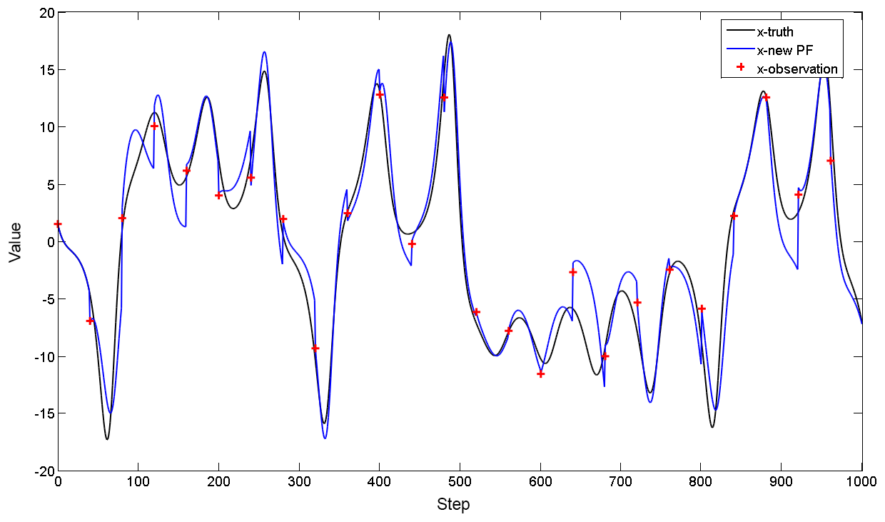
Figure 1Results of the new PF for the Lorenz-63 model of the x component. The red crosses are observations, the black line is the true state and the blue line represents the new PF results.

Download

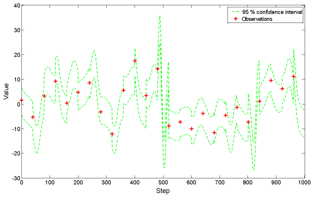
Figure 2The 95 % confidence interval computed by posterior particles. The green dashed lines denote the upper and lower limits of the interval and the red crosses are observations.

Download

Figure 1 shows the results of the x component using the new PF with 20 particles. Note that the new PF procedure is close to the truth with much fewer particles, which is more efficient than the standard PF procedure with hundreds of particles. Compute the confidence interval with the 95 % level using the posterior particles every step. Figure 2 shows that the intervals contain observations at almost all the steps at which observations exist. That means particle sets after translation are closer to observations and true states. The evolution of all particles is displayed in Fig. 3, in which most particles are very close to observations except for several ones at moments when the state changed obviously. The RMSD sequence is shown in Fig. 4; it tends to be stable when the number of particles is more than 20. This means the improved algorithm only needs no fewer than 20 particles.

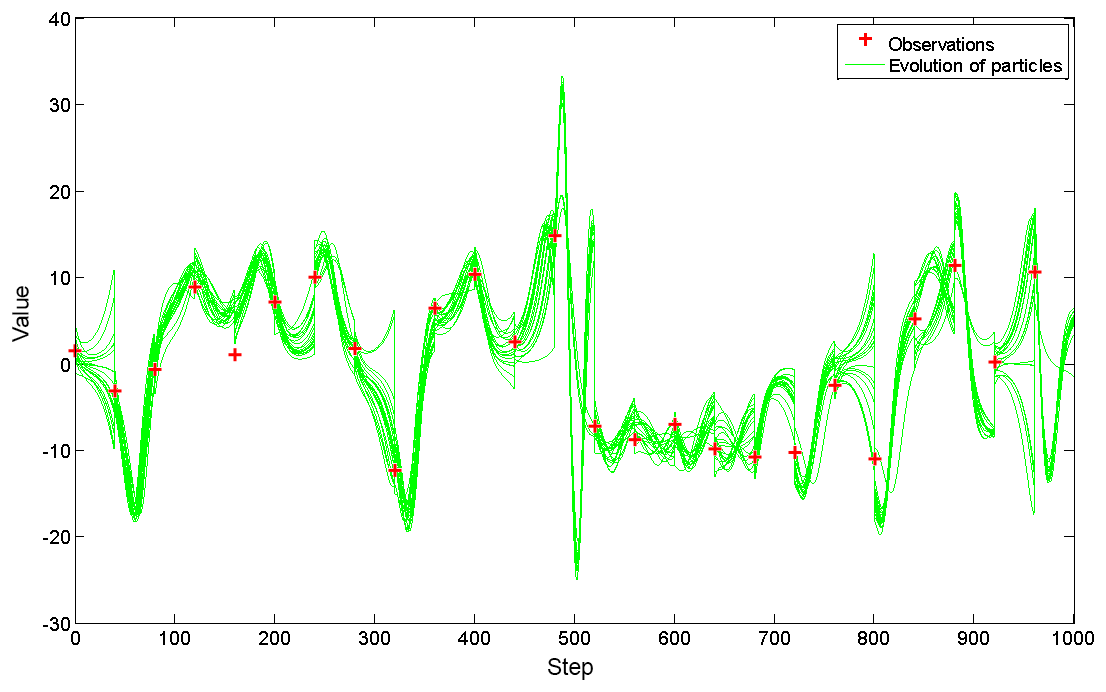
Figure 3The evolution of posterior particles in time. The green dashed lines show the traces of all particles; the red crosses denote the observations.

Download

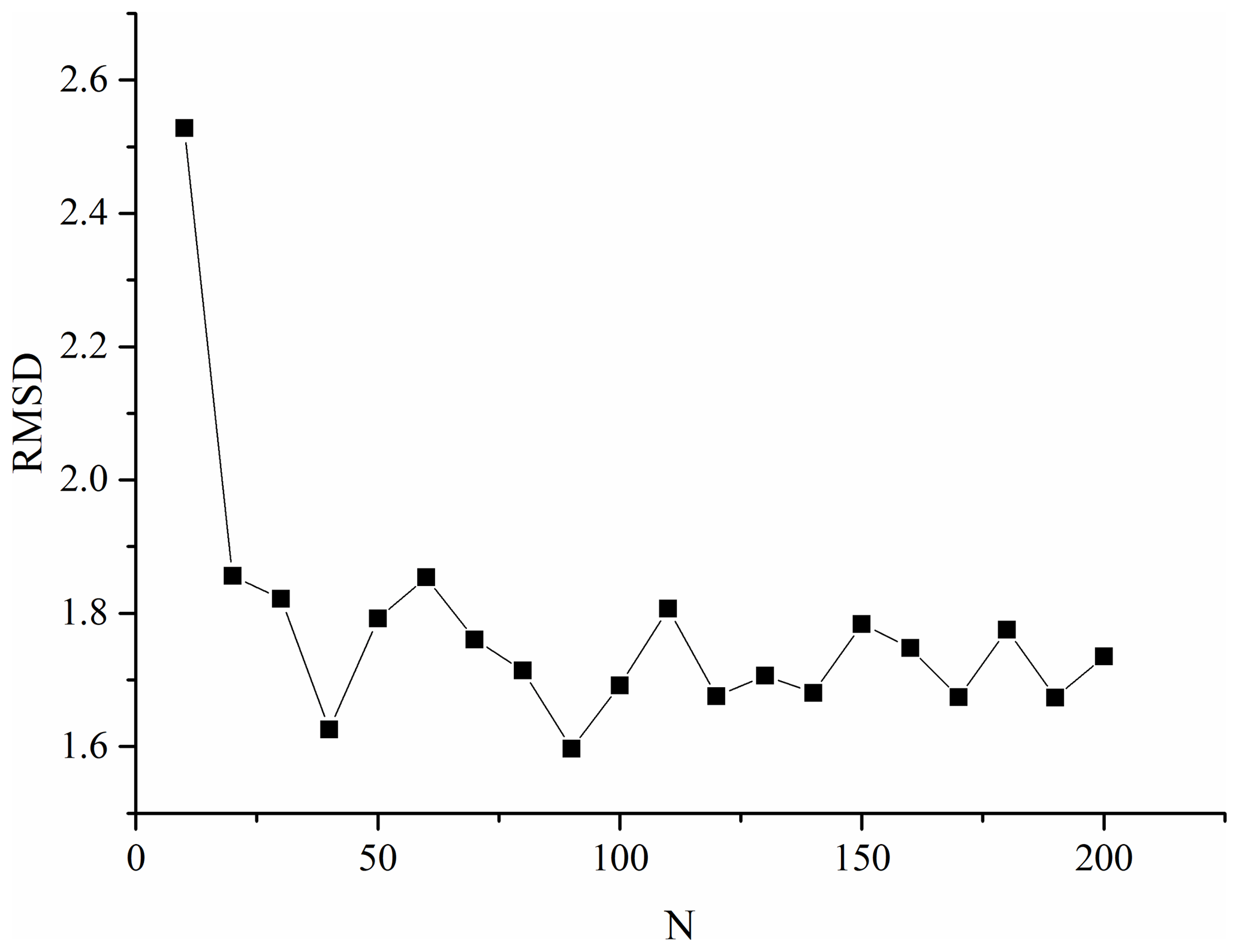
Figure 4RMSD of the estimation with respect to particle numbers. The value is relatively high when the particle number is fewer than 20 and tends to be stable when higher than 20.

Download

TRIGRS is a program modeling rainfall infiltration, using analytical solutions for partial differential equations that represent one-dimensional vertical flow in isotropic, homogeneous materials for simply saturated or unsaturated conditions. It computes changes of rainfall pore pressure and FS with rainfall infiltration. The FS is computed using a simple infinite-slope model, cell by cell.

In this experiment, the FS is applied to assimilation. It is calculated as follows:

in which c is soil cohesion, α is slope angle, ϕ is soil friction angle, φ is the groundwater pressure head depending on depth Z and time t, γ_W is groundwater unit weight, and γ_S is soil unit weight at saturation.

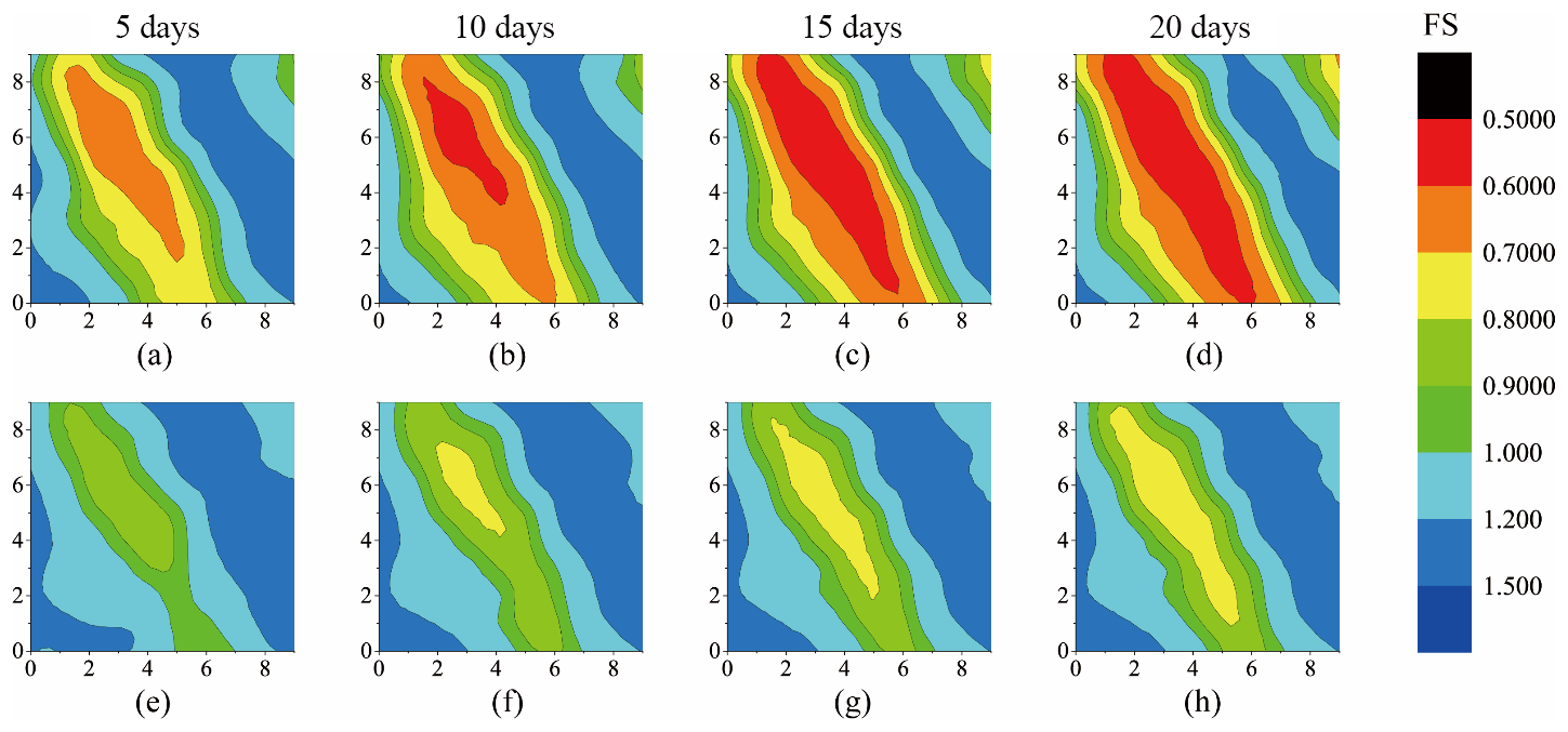
Figure 5Model results and assimilation results of FS. The maps in the first row are the model running for 5, 10, 15 and 20 days, and those in the second row are the assimilation results. The horizontal and vertical coordinates in each graph are the grid numbers of each cell.

Download

An example of the 10×10 grid TRIGRS model is set to be the background, and each grid is a square with a length of 10 m. The simulated observations are generated from the FS by adding a disturbance with normal distribution N(0.2, 0.3). Due to the difficulties of determining the parameter φ, the soil friction angle and its high sensitivity to results, we now generate a set of particles $\left\{{\mathit{\phi }}_k^i\right\}$ to form φ, in which k and i are indices of step and particle number, respectively. The input model variance of φ is 2 and observation variance of FS is 0.3. At each step, φ and FS will be updated, and the updated parameters continue to participate in the next step of operation as initial parameters. The number of particles is set to 20 in the PF program. Figure 5 shows the model running results and the assimilated results of the FS running for 5 days, 10 days, 15 days and 20 days. In the model running results, the value of FS is smaller and decreases rapidly, while in the assimilated results the change is relatively gentle.

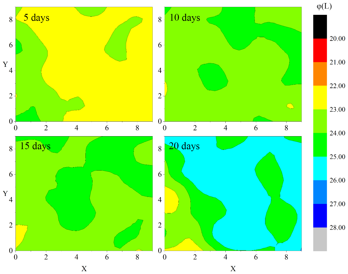
Figure 6The distribution variation in groundwater pressure head (φ) with assimilated time. The horizontal and vertical coordinates in each graph are the grid numbers of each cell.

Download

To evaluate the distribution variation in φ, we propose that the estimation of φ is calculated as formula

in which $w_k^i$ is calculated using Eqs. (18) and (19). Figure 6 shows the distribution variation in φ running for 5 days, 10 days, 15 days and 20 days. Actually, the estimation of φ uses the same method and particles of the estimation of FS. Figure 6 shows the distribution variation in φ running for 5 days, 10 days, 15 days and 20 days. The change of φ estimation in a single cell is illustrated in Fig. 7, considering the middle unit, grid cell (5, 5).

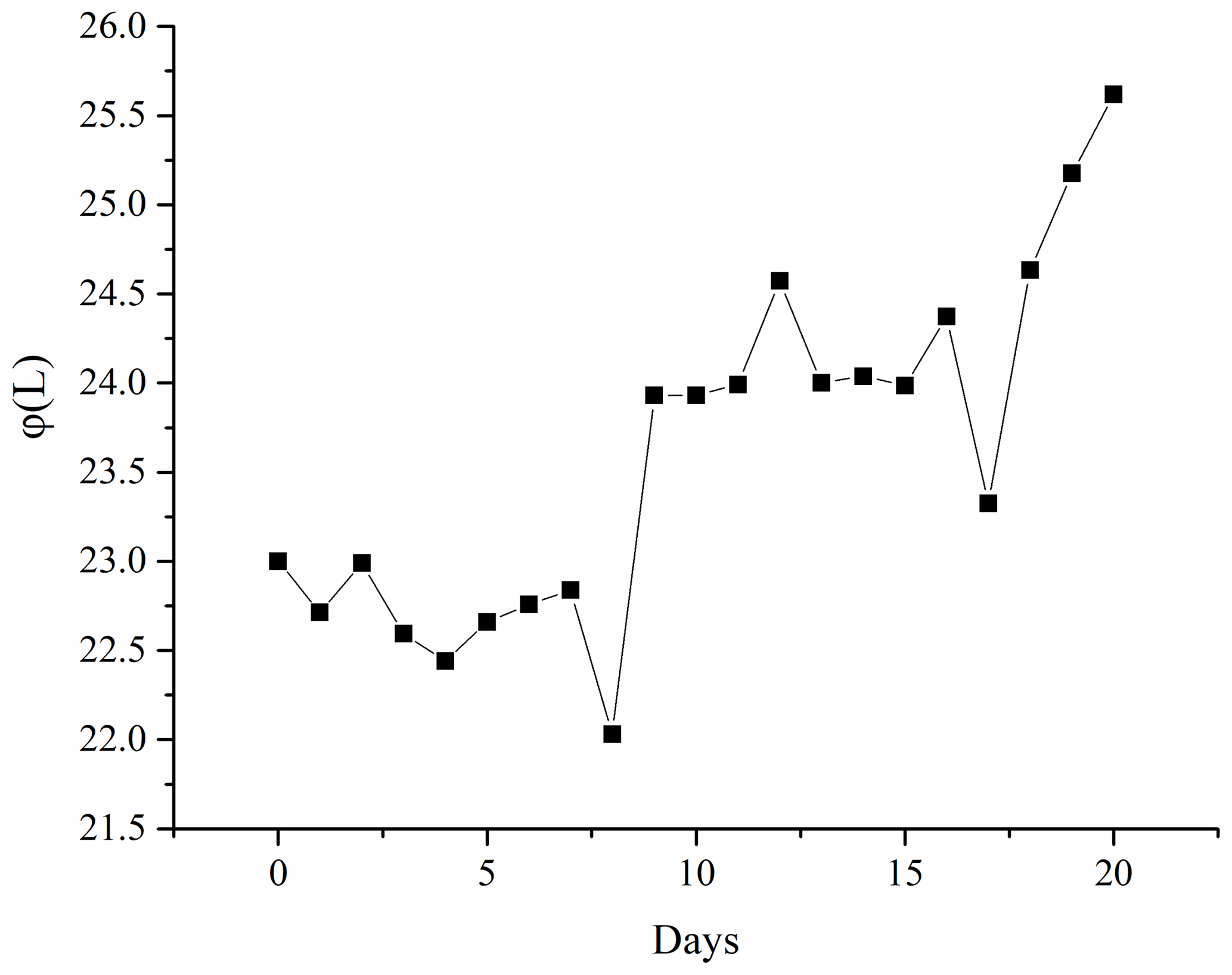
Figure 7The changing line of the groundwater pressure head (φ) estimation of grid cell (5, 5) with assimilation time. The value grows with the evolution of the landslide.

Download

To assess estimations of all grid cells, the RMSD of the whole grid of points to measure the estimated error is modified to

where N_p is the total number of grid points, and i and j are the indices of the row and column number, respectively. The RMSD curve with assimilating days is shown in Fig. 8, which suggests the value is large on the first 2 days of initialization, fluctuates in the next days and is steady when there are no observations.

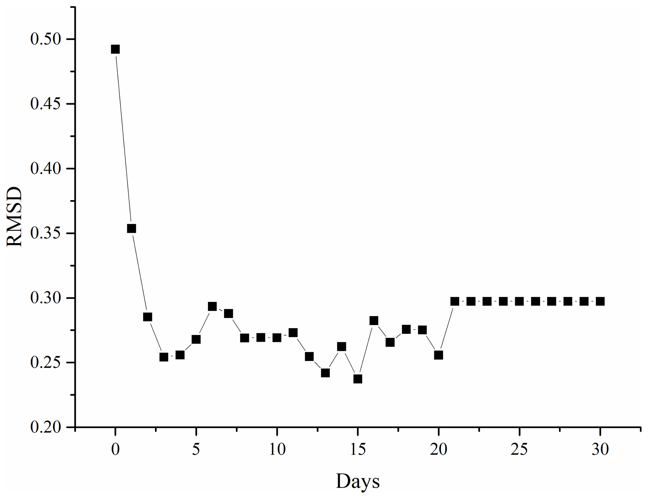
Figure 8RMSD line of all grids depending on assimilation time. The TRIGRS model is assimilated with observations in the first 20 days, and results of days 21–30 are model running results without observations assimilated.

Download

The data in this experiment are mainly collected by observation or generated by simulation. Data sets and figures have been uploaded to the Supplement. The model information and program of TRGIRS are obtained from https://pubs.usgs.gov/of/2008/1159/ (US Geological Survey, 2017).

The supplement related to this article is available online at: https://doi.org/10.5194/nhess-18-2801-2018-supplement.

CX conceived the idea of this article and completed the paper. GN proposed some important suggestions of algorithm applications in the TRIGRS assimilation. Validation of the algorithm, chart sorting and editing were completed by HL and JW.

The authors declare that they have no conflict of interest.