the Creative Commons Attribution 4.0 License.
the Creative Commons Attribution 4.0 License.
 | 02 Nov 2018
Wave run-up prediction and observation in a micro-tidal beach
Diana Di Luccio
Guido Benassai
Giorgio Budillon
Luigi Mucerino
Raffaele Montella
Eugenio Pugliese Carratelli
Extreme weather events bear a significant impact on coastal human activities and on the related economy. Forecasting and hindcasting the action of sea storms on piers, coastal structures and beaches is an important tool to mitigate their effects. To this end, with particular regard to low coasts and beaches, we have developed a computational model chain based partly on open-access models and partly on an ad-hoc-developed numerical calculator to evaluate beach wave run-up levels and flooding. The offshore wave simulations are carried out with a version of the WaveWatch III model, implemented by CCMMMA (Campania Centre for Marine and Atmospheric Monitoring and Modelling – University of Naples Parthenope), validated with remote-sensing data. The waves thus computed are in turn used as initial conditions for the run-up calculations, carried out with various empirical formulations; the results were finally validated by a set of specially conceived video-camera-based experiments on a micro-tidal beach located on the Ligurian Sea. Statistical parameters are provided on the agreement between the computed and observed values. It appears that, while the system is a useful tool to properly simulate beach flooding during a storm, empirical run-up formulas, when used in a coastal vulnerability context, have to be carefully chosen, applied and managed, particularly on gravel beaches.


Real-time forecast and hindcast systems for ocean and coastal risks are becoming more and more common; the availability of both global and regional weather and sea state modelling systems has put the development of warning systems within reach of local authorities and engineering companies. Such systems, however, are generally aimed at providing real-time evaluation of damage to coastal infrastructure or dwellings rather than of risks of beach flooding. Assessing and forecasting such hazards is an ever increasing concern, especially in areas where seaside tourism is an essential part of the economy, as for instance in most Mediterranean countries. Although in recent years a large number of papers have been published on the validation of offshore numerical models, to the best of our knowledge very few studies have been published on the development and the application of operational models including the effects on beaches; hence this paper is aimed at validating a whole chain of models to simulate the action of waves, starting from wind and offshore wave formation, through wave propagation, down to the final segment, which involves the analysis of set-up and run-up on the coast. In particular, a specially conceived experimental set-up has been prepared for the final stage, i.e. flooding of the beach. In the following, the state of the art of each component of the model chain will be very briefly discussed, while some more detail will be provided on the wave run-up and beach flooding and on related experimental techniques.
The computation of winds and offshore waves is a well-settled field, in relation to both the research and operational procedure (Benassai and Ascione, 2006a; Bertotti and Cavaleri, 2009; Cavaleri and Rizzoli, 1981; Mentaschi et al., 2013). Also, the assimilation of wave measurements is a well-tested technique (see for instance Bidlot et al., 2002).
The monitoring and forecasting of wind–wave interaction processes is however particularly critical along coastal areas, which are highly dynamic, complex systems that respond in a non-linear manner to external perturbations: for instance, coastal vulnerability has been considered by many researchers (Didenkulova, 2010; Di Luccio et al., 2017; Di Paola et al., 2014), also taking into account sea-level rise (Benassai et al., 2015a) and subsidence (Aucelli et al., 2016). Measurements are often difficult: satellite data do not reach the adequate resolution and quality when approaching the coast (Aulicino et al., 2018; Cotroneo et al., 2016). The quality of predicted wave data depends on the quality of driving wind fields (Rusu et al., 2014), which are normally provided by global forecasting models, satellite altimeters (Benassai et al., 2015b; Reale et al., 2018) or alternatively by satellite-based microwave synthetic aperture radar (SAR) (Johannessen and Bjorgo, 2000). Much work has been done on the reliability of these data sources and their application is now common practice (Benassai et al., 2013a, b, 2018; Dentale et al., 2018).
We focused our attention on wave run-up prediction; wave run-up prediction is required in most coastal vulnerability and risk evaluation projects (Didenkulova and Pelinovsky, 2008; Didenkulova et al., 2010). Wave run-up (Ru) is defined as “the landward extent of wave uprush measured vertically from the still water level” (Melby et al., 2012). Although complex numerical models are required (Dodd, 1998; Hubbard and Dodd, 2002) to provide accurate estimates of wave run-up with given boundary conditions, simplified run-up formulas are useful to give realistic results on existing cross-shore profiles. The earliest formulation of run-up height was provided in the study of Hunt (1959), who calculated run-up from incident regular waves. He provided the following equation (here, as in most empirical formulas, Ru includes the wave set-up):
where ξ is the Iribarren number or surf similarity parameter (Battjes, 1975)
β is the beach slope angle, H0 is the deep-water significant wave height and L0 is the linear theory deep-water wavelength (Airy, 1841)
where T is the wave period.
Holman (1986) measured extreme value statistics of wave run-up on a shoreline from a single beach and correlated them with the offshore Iribarren number. Mase (1989) performed an extensive series of laboratory tests for the prediction of run-up elevations of random waves on gentle smooth and impermeable slopes as a function of the surf similarity parameter. He included irregular waves and statistical values of the obtained run-up levels, that is Rumax (the highest run-up elevation), Ru2 % (the run-up elevation which is exceeded by 2 %), Ru10 % (the run-up elevation which is exceeded by 10 %), Ru33 % (the run-up elevation which is exceeded by 33 %) and Rumean (the average of the total run-up elevation) (van der Meer et al., 2016). He also introduced two coefficients which are dependent on the characteristic run-up level.
Stockdon et al. (2006) extended the work of Holman (1986) to several beaches covering a wide range of offshore wave conditions to derive a parametric predictor of the total run-up height. They considered the run-up level Ru2 % to be a function of the two different contributions of wave set-up and swash.
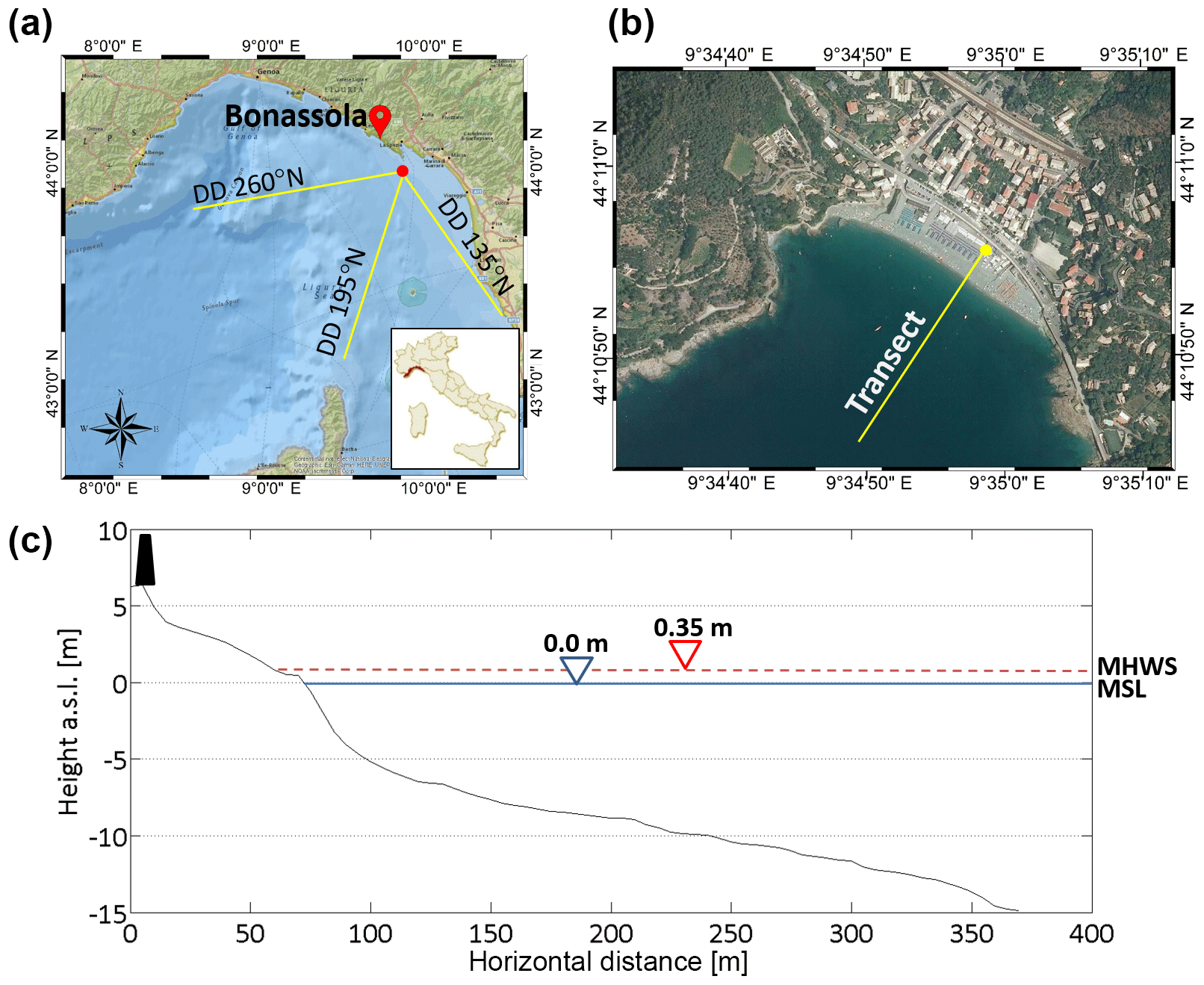
Figure 1Bonassola beach study area with (a) the location of the La Spezia SWAN buoy (red circle) and the main and secondary fetches (image source: National Geographic); (b) the monitored cross-shore transect with video camera system location (yellow circle) (image source: http://www.pcn.minambiente.it/mattm/servizio-wms/, last access: 15 June 2018); (c) the beach profile along the transect with the location of the anthropic structures (black trapezium), mean sea level (MSL) and the mean spring tidal range (MHSW) was extracted by the official Italian tide archives (http://www.mereografico.it, last access: 4 December 2017).
Poate et al. (2016) demonstrated that wave run-up on gravel beaches under energetic wave conditions was significantly under-predicted by the Stockdon et al. (2006) equation and proposed a new run-up parametrization for (pure) gravel beaches. They made clear that on sandy beaches under extreme waves, run-up conditions become dominated by infragravity waves (Guza and Thornton, 1982; Senechal et al., 2011) with the incident storm waves breaking and dissipating their energy further offshore, whereas on gravel beaches very large waves can impact directly on the beach.
Video recording observations of run-up on a wide range of storm wave conditions was performed, among others, by Ruggiero et al. (2004) and Bryan and Coco (2007), who collected vertical run-up elevation time series using the “timestack” method (Aagaard and Holm, 1989; Holland and Holman, 1993). Since then, a number of run-up measurements using remote video imagery of the beaches have been carried out. Further work along this line was carried out by Stockdon et al. (2007), who calculated wave run-up elevation and set-up from modelled offshore wave conditions using SWAN (Sea Wave Measurement Network) and an empirical parametrization (Stockdon et al., 2006) for the evaluation of coastal vulnerability and run-up elevation. In the last few years the USGS National Assessment of Coastal Change Hazards project has been working in collaboration with the National Oceanic and Atmospheric Administration (NOAA)/National Weather Service (NWS) and the National Centers for Environmental Prediction (NCEP) to produce total water level and coastal change forecasts (https://coastal.er.usgs.gov/hurricanes/research/twlviewer/, last access: 1 January 2018). This operational model combines NOAA wave and water level predictions and a USGS wave run-up model with beach slope observations to provide regional weather offices with detailed forecasts of total water levels (Doran et al., 2015; Stockdon et al., 2012). Following Paprotny et al. (2014), forecasts of wave run-up on two beaches of the Polish Baltic Sea coast were tested to evaluate flooding, by chaining the WAM wave model with run-up empirical formulas during SatBałtyk-Shores Operating System.
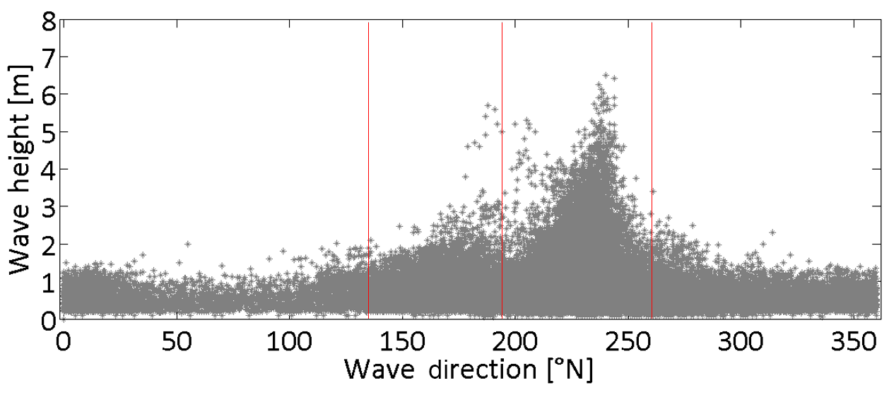
Figure 2Significant wave heights and wave directions recorded from the SWAN buoy of La Spezia 1989–2009. Red lines mark the sectors of the waves' origin: 195–260∘ N (the main fetch) and 135–195∘ N (the secondary fetch).
In this paper wave run-up levels were computed with the various different formulations described above. Since no local measurements from buoys were available (Montella et al., 2008), a version of the WaveWatch III (WW3) model was used, as implemented by the Campania Centre for Marine and Atmospheric Monitoring and Modelling (CCMMMA) – University of Naples Parthenope, by making full use of a high-spatial-resolution weather-ocean forecasting system with a high-performance computing (HPC) system for simulation and open environmental data dissemination (Montella et al., 2007). This deep-water numerical model (Ascione et al., 2006) was coupled with a wave propagation model in shallow water, which provided the run-up evaluation on the beach. This model chain was tested on a micro-tidal beach located on the Ligurian Sea in order to assess the reliability of the wave modelling system, already verified in offshore conditions by means of in situ and remote-sensing techniques (Benassai and Ascione, 2006b; Carratelli et al., 2007; Reale et al., 2014).
This paper is organized as follows: the field data and the numerical models are reported in Sects. 2 and 3 and the results and validation are given in Sect. 4. Lastly, our discussion and the conclusions are reported in Sects. 5 and 6, respectively.
The experiments presented in this paper were carried out on the Bonassola beach (La Spezia, Italy), which is approximately 410 m long and is located on the eastern coast of Liguria. The coastline is oriented south-east to north-west and it is exposed to waves coming from the south-west (215–245∘), while it is protected from the south-east waves. Bonassola beach can be classified as a mixed gravel–sand (MSG) beach due to its sediment characteristics and its morphology (Jennings and Shulmeister, 2002). The range of mean sediment grain size in the swash zone is 0.76 to 62.65 mm (0.38 to −5.96ϕ). The mean beach slope is approximately 8.3 % from the shoreline to 10 m in water depth and becomes 5.5 % between 10 and 30 m (Fig. 1c). The offshore beach is made up of a mixture of mean and coarse sand. The data of the grain size and the slope of the beach were taken from a geomorphological survey conducted by the University of Genoa in 2012 and reported in Balduzzi et al. (2014).
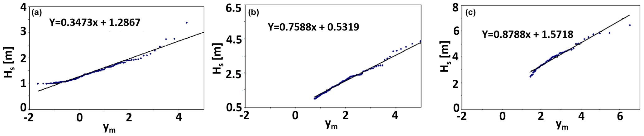
Figure 3Matching between the recorded extreme wave heights and the reduced variable for the Gumbel distribution function for waves coming from (a) 135–195∘ N, (b) 195–225∘ N and (c) 225–260∘ N. The dataset is relative to the records of the La Spezia wave buoy in the period 1989–2009.
The offshore wave climate was estimated by using the data recorded by the Italian RON (Italian National Wavemeter System) buoy located offshore of La Spezia ( N, E) from 1989 to 2009. The main fetch sector is comprised between 195 and 260∘ N while the secondary fetch is limited between 135 and 195∘ N (in the following S1). The main transverse sector was then subdivided into two sub-sectors, 195–225∘ N (S2) and 225–260∘ N (S3), in which two different wave conditions were observed: the maximum significant wave height (Hs) is lower than 5.5 m between 195 and 225∘ N and higher than 5.5 m between 225 and 260∘ N (Fig. 2).
A representative sample of statistically independent extreme wave events N was selected on the basis of the peak-over-threshold method (Goda, 1989). The 48 h maxima based on over-threshold H* time series have been sorted in order to find the best fit between the data and the Gumbel (Fisher–Tippet type I) cumulative probability distribution function.
where A is the location parameter and B is the scale parameter. A rank index m, ranging from 1 to N, was associated with the order of the array and the sample rate of non-exceedance was calculated as
and it is assumed coincident with the non-exceedance probability.
Figure 3 shows the rate between and the relative reduced variable for waves coming from each directional sector.
The linear regression line is given as
where A (slope of the regression line) and B (line intercept) coefficients are linked with the probability distribution function. The significant wave height Hr with return period Tr can be determined by the following expressions:
where the relative reduced variable is
and the sample intensity λ is defined by the ratio between the number of extreme events and the number of years of observation. Table 1 gives the offshore wave height Hr obtained for each directional sector as a function of the relative return period Tr; it is found that the maximum Hr>5.0 m is to be found in sector S3 (the western directions).
Table 1Design waves, in terms of Hr associated with different return periods (Tr equal to 1, 5, 10, 20, 50 and 100 years), obtained from the La Spezia buoy (1989–2009) for each directional sector (S1, S2 and S3).
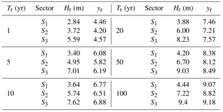
In order to test the performance of the system, we thus considered a western storm event with a return period of less than 1 year, i.e. with significant wave heights that can occur several times a year.
3.1 Wave numerical simulations
The weather–sea forecasting tool (Fig. 4) was implemented by CCMMMA using an HPC infrastructure to manage and run a modelling system based on the open-source numerical models Weather Research and Forecasting (WRF) (Skamarock et al., 2001) and WaveWatch III (WW3) (Tolman, 2009) organized in a workflow. The operational system is based on complex data acquisition, processing, simulation, post-processing and inter-comparison dataflow, provided by the FACE-IT workflow engine (Pham et al., 2012), which is available open source and as a cloud service. This integrated data processing and simulation framework enables (i) data ingestion from geospatial archives; (ii) data regridding, aggregation and other processing prior to simulation; (iii) making use of high-performance and cloud computing; and (iv) post-processing to produce aggregated yields and ensemble variables needed for statistics and model testing. The main workflow tool is the WRF numerical model, which computes the 10 m wind fields and other atmospheric forcing needed to drive the WW3 offshore wave model, which in turn yields the initial and boundary conditions for the shallow-water wave simulation of wave transformation and run-up. Wave simulations were carried out using the WW3 model version 3.14, a third-generation wave model developed at NOAA/NCEP. The physics packages used in the our implementation are as follows.
-
We used the linear input parametrization of Cavaleri and Rizzoli (1981) with a filter for low-frequency energy as introduced by Tolman (1992). The source term package of Tolman and Chalikov (1996) has been implemented with the stability correction.
-
We used the discrete interaction approximation (DIA) (Hasselmann and Hasselmann, 1985) for non-linear wave–wave interactions.
-
We used the ULTIMATE QUICKEST propagation scheme (Leonard, 1979) with the averaging technique for the “garden sprinkler” alleviation Tolman (2002).
-
We used the JONSWAP bottom friction formulation (Hasselmann et al., 1973) with no bottom scattering and Battjes and Janssen (1978) shallow-water depth breaking with a Miche-style limiter.
In order to produce the numerical simulations presented in this paper, we configured the WW3 model with two one-way nested computational domains.
-
Coarse domain d01 covers almost the whole Mediterranean Sea by a grid of 608×203 points spaced at a 0.09∘ resolution (long∘ W, long E; lat∘ N, lat N). d01 is thus as a closed domain forced only by the weather conditions provided by the WRF offline coupled data; no wave boundary conditions are therefore to be provided for this domain.
-
Fine domain d02 covers the seas around the Italian peninsula at a grid of 486×353 points spaced by a 0.03∘ resolution (long∘ E, long∘ E; lat∘ N, lat∘ N). In the used WW3 model configuration, d02 is coupled online with the d01 domain.
The outputs from the model include gridded fields with the associated significant wave height (Hs), wave direction (Dirmn), mean period (Tm) and spectral information. The WW3 grid points close to the coast were used as a “virtual buoy” (VB), providing the data needed to compute the wave transformation down to the coast, with the final goal of simulating the run-up parameter on the beaches.
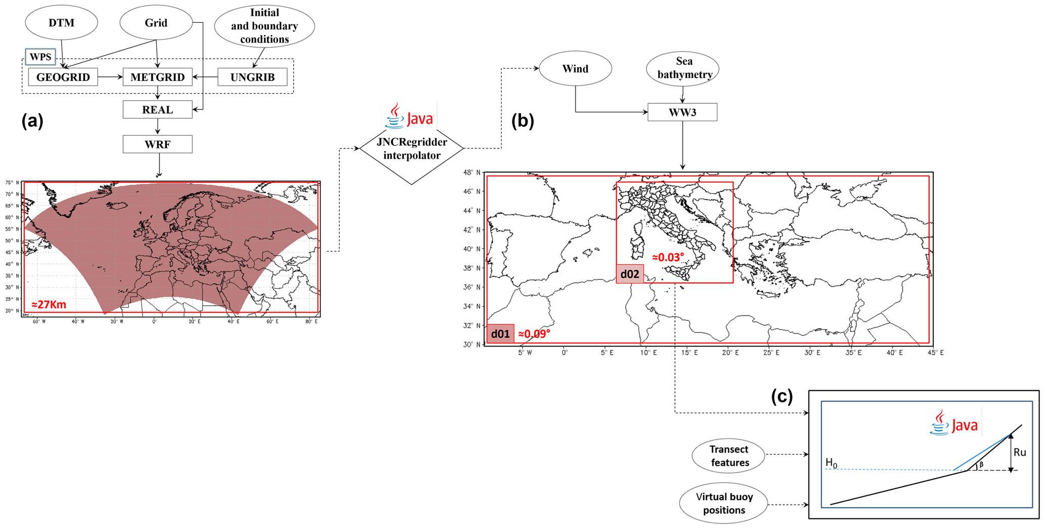
Figure 4Model chain from the atmospheric model WRF (a) to the offshore wave model WW3 (b) and the run-up calculator (c). The block diagram shows evidence of the input–output components of the model coupling data flux.
3.2 Wave run-up calculator
The last software component of the coupled model chain reported in Fig. 4c is the wave run-up calculator on the beach. We used a one-dimensional approach to simulate the beach run-up with a Java software designed to be highly modular as a part of the operational forecasting system. The wave condition in the VB (Hs, Tm and Dirmn) and the beach slope β or βf derived from a cross-shore beach profile (for example the one shown in Fig. 1) represent the inputs to resolve the run-up empirical equations.
Dealing with random waves, Rux % is defined as the wave run-up level, measured vertically from the still-water line, which is exceed by x % of the number of incident waves (van der Meer et al., 2016).
Holman (1986) proposed an empirical formula to obtain Ru2 %, based on the Iribarren number ξf constrained with surf zone slope angle:
In detail, H0 is the deep-water significant wave height, which can be related to the value at the VB through the ratio of the respective wave celerity to (Shore Protection Manual, 1984):
For the VB the wavelength is equal to , in which k is the wave number obtained by the Hunt approximation of the standard dispersion relation (Fenton and McKee, 1990):
where dn are six constant values given by Fenton and McKee (1990), and σ is the wave frequency.
Mase (1989), on the basis of laboratory tests, obtained the characteristic run-up level Rux % as a function of two empirical coefficients a and b.
Mase (1989) suggest a=1.86 and b=0.71 for Ru2 %, a=2.32 and b=0.77 for Rumax, a=1.70 and b=0.71 for Ru10 %, a=1.38 and b=0.70 for Ru33 %, and a=0.88 and b=0.69 to obtain Rumean.
Stockdon et al. (2006) considered the run-up Ru2 % to be a function of two separate terms to consider the different contributions of the wave set-up and swash (the latter term on the left-hand side)
where βf is the average slope over a region ±2σ around 〈η〉, and σ is the standard deviation of the water level elevation η(t). In random waves, H0 is substituted by the spectral wave height Hm0=4(m0)0.5, defined as the incident significant wave height in shallow water, where m0 is the zeroth spectral moment.
Poate et al. (2016) proposed the following equation, specifically developed for gravel beaches:
where C is a constant fixed to 0.49 (Poate et al., 2016).
The mean beach slope β and the foreshore beach slope βf, used in the run-up equations are calculated taking into account the examined cross-shore beach profile. Equation (14) has been used by a number of researchers to compute coastal inundation and consequently coastal vulnerability and risk (Benassai et al., 2015a; Di Paola et al., 2014). Melby et al. (2012) compared the skill of some different run-up models through some statistical measures and introduced a new statistical skill measure, described in Sect. 3.3.2, which was used to compare the different formulations for an extensive dataset. In the following, we compared the different run-up equations through the deviation from the observed run-up levels evaluated with video camera records. Among the different empirical formulas used to calculate the wave run-up parameters, Eqs. (10), (13), (14) and (15) have been used to obtain run-up time series. In particular, the Holman (1986), Mase (1989), Stockdon et al. (2006) and Poate et al. (2016) formulas have been used for the 2 % wave run-up levels, while only the Mase (1989) equation has been used to calculate the 10 %, 33 %, mean and max run-up levels.
3.3 Waves and beach run-up observations
3.3.1 Altimeter and video monitoring
Satellite altimeter data provide a large spatial coverage over the entire region of the central and northern Tyrrhenian Sea, which cannot be accomplished by in situ observations at fixed stations. The offshore part of the model system was therefore validated by making use of remotely sensed data, obtained from the dataset of the Ocean Surface Topography Mission (OSTM/Jason-2), launched on 20 June 2008. Figure 5 shows the considered track of the OSTM/Jason2 satellite. Geophysical Data Record (GDR) provides Ku-based significant wave height data with a spatial resolution of 11.2 km (along track) × 5.1 km (across track).
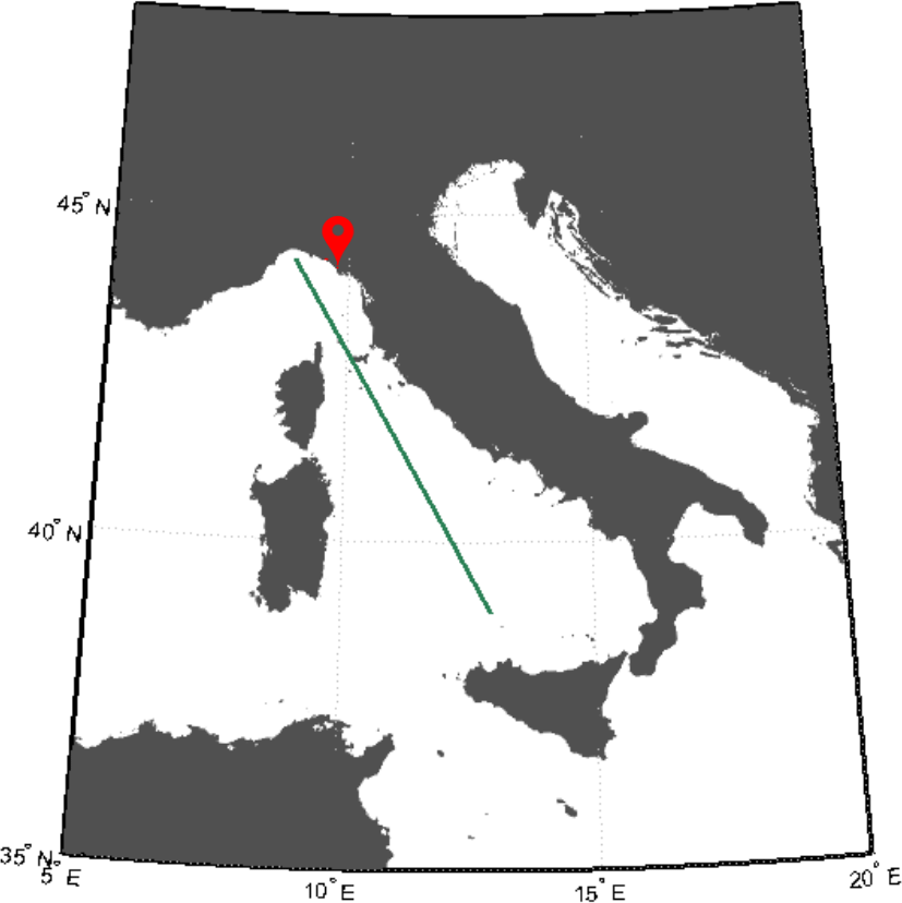
Figure 5Map showing the WRF and WW3 models' spatial domains including the Italian peninsula overlapped with the location of the video camera system (red marker) and the used OSTM/Jason-2 satellite dataset (green line).
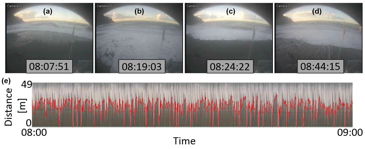
Figure 6A time sequence (a), (b), (c), (d) of the Bonassola beach sea storm recorded by camera from 08:00 to 09:00 UTC on 10 February 2016; (e) timestack obtained by analyzing the video camera acquisitions in the time interval from 08:00 to 09:00 UTC relative to 10 February 2016, highlighting with a red line the detected run-up value.
The beach run-up simulations, carried out with the various equations reported above, were validated by means of a video monitoring system placed in the middle of Bonassola beach (Fig. 6a, b, c, d). Video recordings of run-up were made using three video cameras, installed at an elevation of about 13 m above mean sea level (m.s.l.), which have allowed complete coverage of the beach since 19 November 2015. The light intensity of each pixel in the cross-shore transects was digitized by using the geometric transformation between ground and image coordinates. Vertical run-up elevation time series were extracted from video recordings using the timestack method (Aagaard and Holm, 1989; Holland and Holman, 1997). This methodology, giving rise to the signal reported in Fig. 6e, is described in the extensive literature on coastal video monitoring (Ojeda et al., 2008; Takewaka and Nakamura, 2001; Zhang and Zhang, 2008). According to Vousdoukas et al. (2012b), the run-up excursion was identified by using the threshold method supplied by Otsu (1975), which is able to identify the wet–dry boundary by pixel colour. The elevation of detected horizontal position (red line in Fig. 6e) was calculated using average slope profile obtained from topographic surveys conducted on Bonassola beach. The run-up position at each video sample time (1 Hz) was obtained with Beachkeeper plus (Brignone et al., 2012), a software based on the MATLAB® algorithm used to analyse the images without any a priori information of the acquisition system. Run-up results have been validated through geo-rectification of camera images, which was performed by using nine ground control points (GCPs). The x–y coordinates of GCPs were acquired in UTM32-WGS84 using differential GPS, with 0.15 m accuracy at the horizontal and vertical positions. The cross-shore resolution of the processed timestack images is 0.2 m, equal to the minimum pixel footprint along the monitored transect, in accordance with Vousdoukas et al. (2012a) and Huisman et al. (2011). The best results have been processed with 5 pixel line analysis, reducing backwash and filtration–extra-filtration detection, using the timestack method.
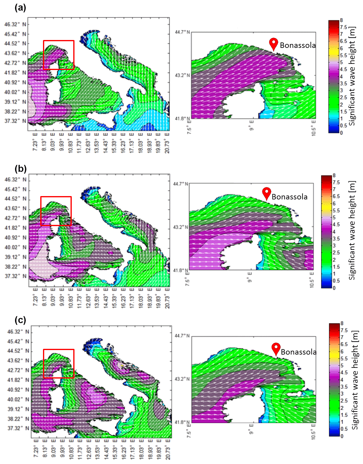
Figure 7Ligurian Sea significant wave height (colour maps) and direction (vector fields) in three moments of sea storm in February 2016. The maps are relative to the WW3 model simulation on 10 February 2016 at (a) 00:00 UTM, (b) 06:00 UTM and (c) 12:00 UTM. Wave height isolines are at 0.5 m intervals.
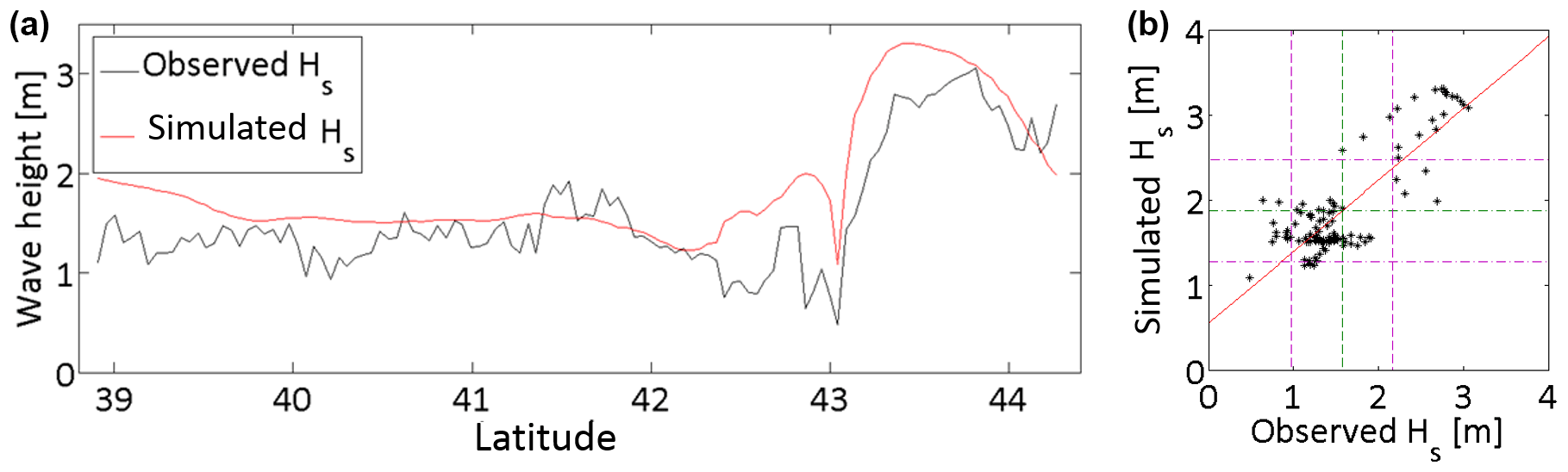
Figure 8Matching between WW3 and Ku-band altimeter data from the JASON-2 satellite pass 44 cycle 280. (a) Time series during the period from 9 February 2016 at 04:58:44 to 05:00:43 UTC. (b) Scatter diagram between observed and simulated Hs (m). The green dotted lines are the mean in the x (1.876) and y (1.574) directions, while the purple dotted lines are the relative standard deviation of 0.6022 and 0.5975.
3.3.2 Comparison statistics
The quality of the results provided by the offshore wave model and by the run-up simulations was evaluated by comparison with wave altimeter records and video camera run-up observations. Deviation of simulated parameters from observed data was estimated through some of the following statistical error indicators proposed by Mentaschi et al. (2013) (Si indicates a simulated variable, Oi indicates an observed variable and N is the number of considered observations):
-
normalized bias (BI)
-
root-mean-square error (RMSE)
-
normalized root-mean-square error (NRMSE)
-
normalized scatter index (SI)
-
linear correlation coefficient (R)
The results are summarized in the summary performance score (SPS) index, based on the RMSE, BI and SI performance, normalized between 0 and 1 (as suggested by Melby et al., 2012).
-
NRMSE performance (NRMSEP)
-
BI performance (BIP)
-
SI performance (SIP)
-
Summary performance score (SPS)
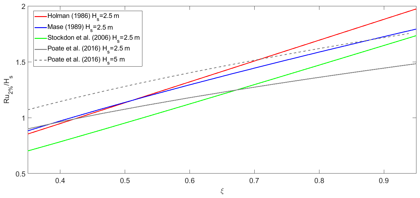
Figure 9Ru2 %∕Hs as a function of the Iribarren number ξ for the different equations with reference to the wave conditions of the February 2016 storm (Hs=2.5 m) and, only for Poate et al. (2016), the same values calculated in more energetic conditions (Hs=5.0 m, dotted line).
In this section some experimental results are presented and discussed to show the capability and accuracy of a wind–wave modelling chain in estimating run-up levels on the beach studied.
4.1 Offshore wave validation with altimeter data
The consistency of the WW3 model was validated taking full benefit of the altimeter data from the OSTM/Jason2 mission, relative to the passage of the satellite during the period from 9 February 2016 at 04:58:44 to 05:00:43 UTC. Figure 7a, b, c depict the simulated WW3 Hs maps on 10 February 2016 at 00:00, 06:00 and 12:00 UTC, with relative zoom, respectively, while Fig. 8 shows the matching between the time history of the measured and modelled offshore Hs along the track.
The results of the wind–wave modelling system were interpolated in both space and time to collocate with the altimeter data. Firstly, hourly WW3 Hs outputs were spatially interpolated (bilinear interpolation) from the grid points to the locations of the altimeter measurements. Interpolations were then carried out in time to fit the satellite pass (linear time interpolation between the previous and following field values). The observed Hs is shown as a blue line in Fig. 8a, while the simulated Hs is reported as a red line. In general, the model fits the measurements quite well, but sometimes it deviates from the observations. For example, the first high-wave event between 41.5 and 42∘ N is underestimated by the model, while the second high-wave event between 43.5 and 44∘ N is slightly overestimated.
It can also be observed that the simulated Hs trace along the satellite track is much smoother than the observations, due to the fact that the WW3 model is incapable of resolving the small scales seen in the altimeter observations (Reale et al., 2013). The statistics of the comparison give an R value of 0.838, a BI of 0.192, a SI of 0.202 and a RMSE value of 0.455 m. The satisfactory agreement is shown by a RMSE lower than 0.46 m and by a correlation coefficient higher than 0.83. In fact, Fig. 8 shows a good match between simulations and observations; however non-negligible differences in terms of Hs can be noted, which can be partially explained taking into account the different spatial gridding resolution scale of modelled (WW3) and remotely sensed (Jason-2) wave estimation products.
4.2 Analysis of the existing wave run-up formulas
In Fig. 9 the run-up Ru2 % normalized with Hs has been reported as a function of the Iribarren number for the different equations considered, in a range of the surf similarity parameter corresponding to dissipative and intermediate beaches (ξ<1.0). The values of βf (used in Holman, 1986, and Stockdon et al., 2006, equations) have been obtained as a multiple N (fixed to 2.25 for convenience) of β (used in Mase, 1989, and Poate et al., 2016, equations). All the equations provide an increase in run-up levels as beaches become more reflective (increase in ξ). In particular, the Holman (1986) and Stockdon et al. (2006) equations exhibit a linear increase as a function of ξ, while the Mase (1989) and Poate et al. (2016) equations exhibit a non-linear one.
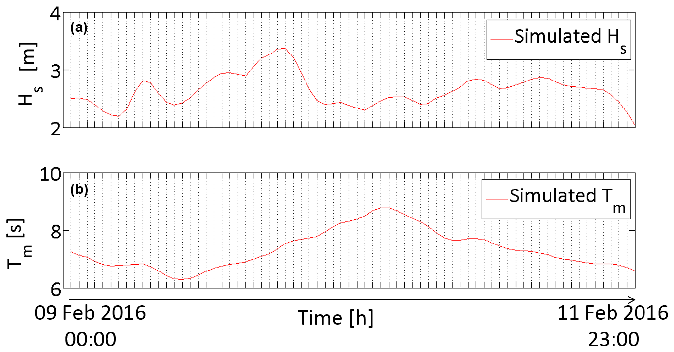
Figure 10Simulated significant wave height (Hs, a) and mean wave period (Tm, b) relative to the 9–11 February 2016 sea storm at the virtual buoy near Bonassola beach. The simulations are carried out using the WW3 model configured with an hourly output time step.
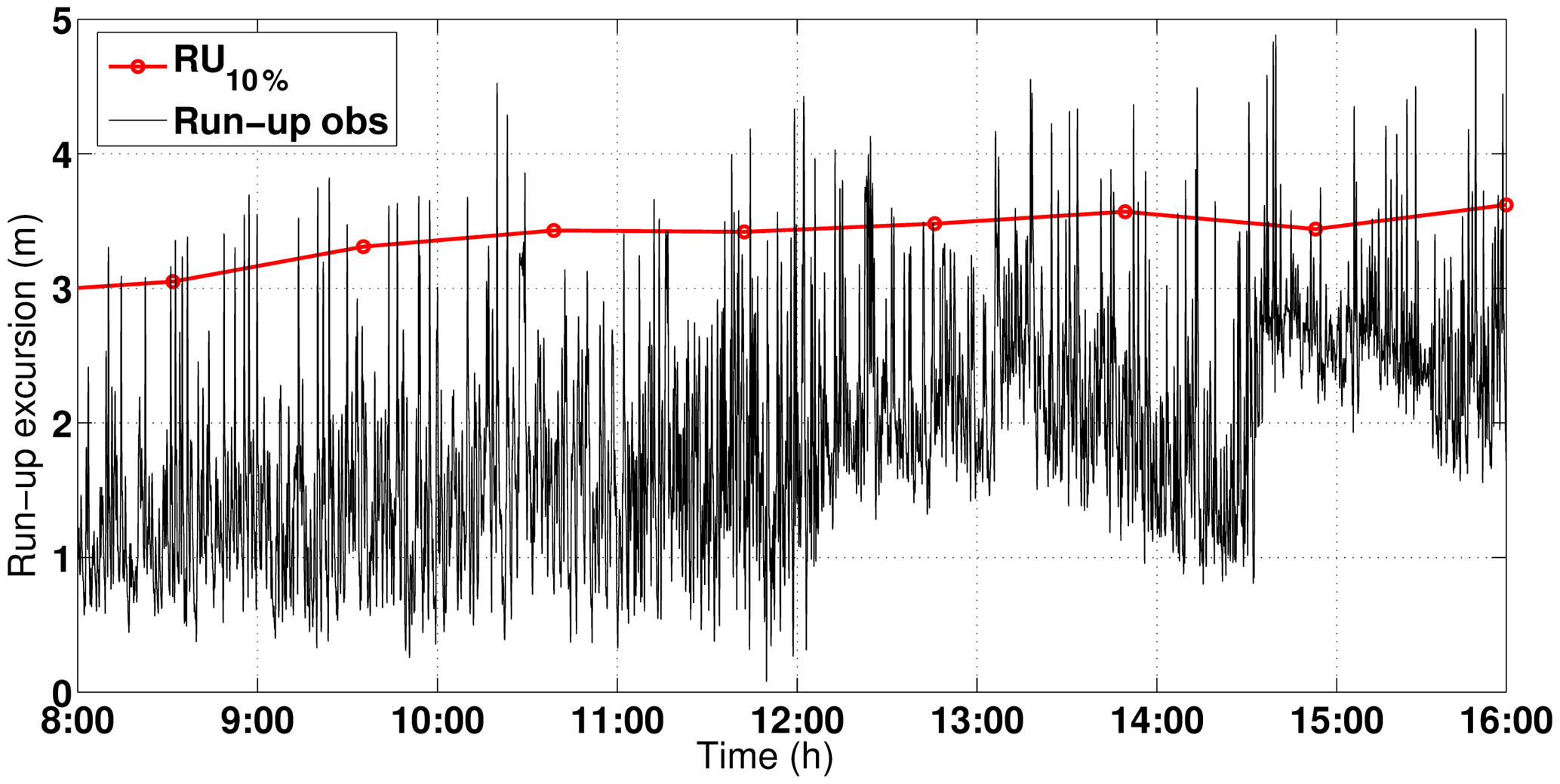
Figure 11Wave run-up levels collected (black line) using pixel timestacks derived from video camera data at Bonassola on 10 February 2016 from 08:00 to 16:00 UTC; Ru10 % trend (red line) as obtained by the timestack analysis at 1 h intervals during the investigated time period.
Table 2Rux % observed with cameras versus Rux % simulated using different equations.
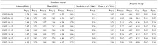
Table 3Statistical error parameters obtained from the comparison between observed and simulated wave run-up levels.
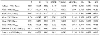
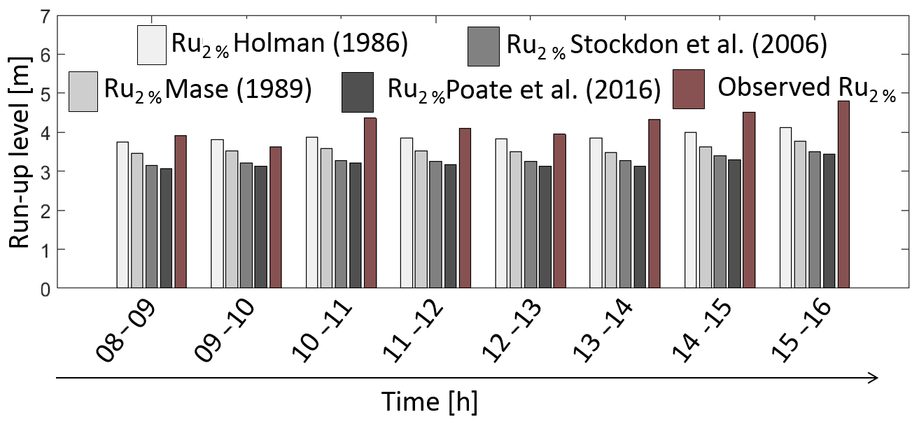
Figure 12Hourly comparison (10 February 2016 from 08:00 to 16:00 UTC) between observed and simulated Ru2 %. The run-up level simulations are carried out using the empirical formulas introduced by Holman (1986), Mase (1989), Stockdon et al. (2006) and Poate et al. (2016).
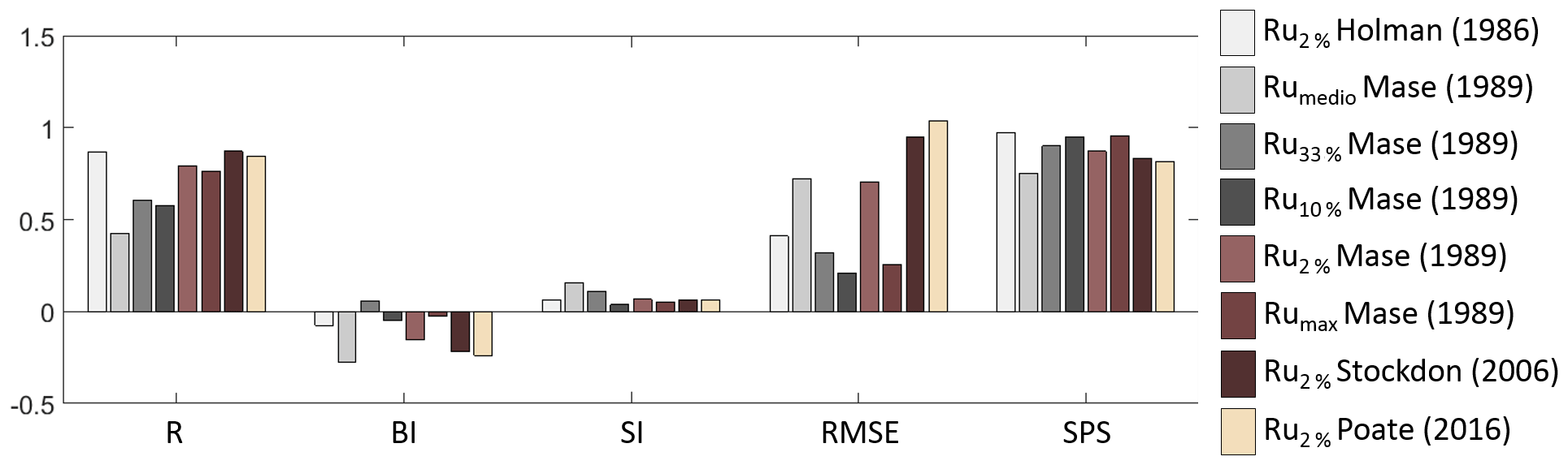
Figure 13Bar diagram of the statistical parameters R (correlation index), BI (bias), SI (scatter index), RMSE (root-mean-square error) and SPS (summary performance score), obtained comparing the run-up video camera observations with the same parameter calculated using the empirical formulas introduced by Holmann (1986), Mase (1989), Stockdon et al. (2006) and Poate et al. (2016).
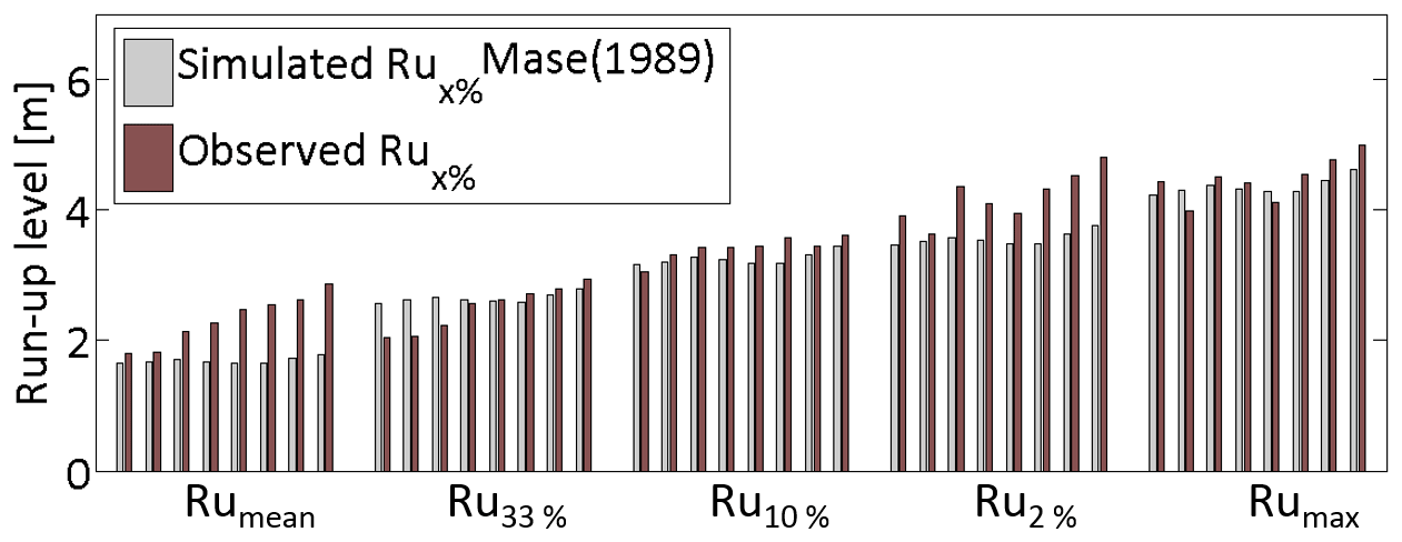
Figure 14Hourly comparison among different Rux % values (Rumean, Ru33 %, Ru10 %, Ru2 % and Rumax) calculated with Mase (1989) equations and observations. The run-up data are relative to the 10 February 2016 sea storm from 08:00 to 16:00 UTC.
With regard to the relative run-up levels, the Holman (1986) and Mase (1989) equations always represent a higher bound for Ru2 %, while the Stockdon et al. (2006) equation is a lower bound, at the least for ξ>0.65.
The Poate et al. (2016) equation is sensitive to Hs: for intermediate storms like the one experienced (Hs=2.5 m) it provides low Ru2 % values, representing a lower bound for ξ>0.65; for severe storms (Hs=5.0 m) it gives higher Ru2 % values compared to the other formulas, providing an upper bound for the run-up (dotted line).
4.3 Wave run-up simulations and validation with the video-monitoring system
In this subsection, wave run-up numerical simulations obtained with the model chain are described with respect to the storm between 9 and 11 February 2016. A preliminary offshore wave simulation was performed on a virtual buoy located offshore of Bonassola beach. The relative Hs and Tm time history is shown in Fig. 10a, b, respectively. The storm exhibited a maximum Hs higher than 3.0 m (with a relative Tm of about 7 s) on 10 February 2016 at 03:00 UTC, followed by a decrease in Hs (with a relative increase in Tm) in the following hours, with values between 2.0 and 3.0 m, in accordance with the regional wave field maps in Fig. 7.
The experimental analysis has been conducted on an average profile, which is provided by beach survey. Since bathymetric and topographic data are subjected to change during storm events, surveys could be repeated after each event to evaluate profile evolution. According to Balduzzi et al. (2014), Bonassola beach is subject to cross-shore sediment movements beyond depth closure and to beach rotation during swell from SE. Therefore, the investigated profile has been selected for a central area in order to avoid excessive coastline changes.
The outcome of run-up assessment showed that the flooding level depends on wave peak period. Despite that wave height is almost unchanged, wave peak period increases by 1.7 s, observed wave run-up increases by 0.5 m and Ru10 % increases from 3.05 to 3.62 m, as reported in Fig. 11.
The run-up formulas described in Sect. 3.2 were evaluated considering the wave conditions of the February 2016 storm event and the cross-shore transect reported in Fig. 1c. The simulation results have been compared with the observed wave run-up elevation time series recorded by a beach camera system on 10 February 2016 from 08:00 to 16:00 UTC. Run-up video records (Fig. 11) were made using the central camera of the video monitoring system described in Sect. 3.3.
The comparison among the different Ru2 % formulas, reported in Fig. 12, shows that the Ru2 % formulas almost always underestimate the levels. In detail, the Holman (1986) results are the highest, followed by Mase (1989), Stockdon et al. (2006) and Poate et al. (2016), in this order. This is consistent with the behaviour of the different formulas evidenced in Fig. 9 for ξ around 0.65 and is confirmed by the RMSE values of 0.41, 0.70, 0.95 and 1.04, respectively, and by the SPS values in decreasing order, 0.92, 0.87, 0.83 and 0.82, respectively (see Fig. 13 and Table 3). The comparison between the hourly mean of the observed and simulated Rux %, obtained using the Mase (1989) equations, reported in Fig. 14, shows more uniform values of the numerical simulations in the 8 h of analysis, due to the lower time resolution of the WW3 model.
In this section, the results of the present study will be discussed, with particular concern for the validation of the offshore and inshore simulations and the operational capability of the modelling chain. The WW3 simulation provided the offshore wave conditions during the examined sea storm, covering the spatial area showed in Fig. 5 (d02 domain). The simulated Hs values, sampled along the green track in Fig. 5, were compared with the altimeter value (OSTM/Jason 2 satellite) through a spatial and temporal interpolation, which introduced some systematic errors; nevertheless, the validation results of the offshore wave simulations with respect to the altimeter data showed a satisfactory agreement with a bias of 0.192 and a standard deviation (SD) lower than 0.6 m. These results slightly overpredicted the measured values, in agreement with the ones of Wahle et al. (2017), who compared SARAL/AltiKa altimeter data with the WAM (WAve Model) simulations.
Conversely, the comparison between the simulated and observed Ru2 % levels on the beach exhibits a general underestimation of the run-up formulas. These discrepancies may be partly attributed to the limited camera resolution in time stack mode, equal to 0.2 pixel, and to a differential GPS accuracy of 0.15 m. Moreover, additional inaccuracies can be linked to the time shift between the model chain output step (1 h) and video recording (1 s), which produces smoother simulated run-up results, as already evidenced in Fig. 14.
The best matching between simulations and observations is given by the Holman (1986) equation, followed by the equations of Mase (1989), Stockdon et al. (2006) and Poate et al. (2016) in this order. This result agrees well with the behaviour of the formulas evidenced in Fig. 9 in the Iribarren range experienced. In particular, this trend is consistent with the behaviour of the Holman (1986) equation, which gives the highest Ru2 % values irrespective of ξ, and with the behaviour of the Poate et al. (2016) equation, which, for the low ξ values experienced, gives a lower bound for Ru2 % for moderate Hs.
The experimental values, in the ξ range considered, are closer to Holman (1986), Mase (1989), Stockdon et al. (2006) and Poate et al. (2016) in this order, in accordance with their RMSE values, which are 0.41, 0.70, 0.95 and 1.04, respectively (see Fig. 13 and Table 3). This is also in agreement with SPS values given in Table 3 and evidences that the Stockdon et al. (2006) equation represents a lower bound limit for Ru2 % in the ξ range lower than 0.65. This is consistent with the considerations of Poate et al. (2016), who noted an underestimation of the Stockdon et al. (2006) equation, which affected the same Poate et al. (2016) equation for moderate wave conditions. Nevertheless, in more energetic conditions, the Poate et al. (2016) equation represents an upper bound for run-up, at least in the range ξ>0.65, as reported in Fig. 9.
This paper has presented the implementation and the results of a numerical model system aimed at forecasting and/or assessing beach vulnerability starting from input data provided by NOAA GFS global wind and computing the wave run-up over the beach through a chain of offline coupled models. The model chain has been validated with a complex set of experiments carried out on a beach in northern Italy, aiming at comparing the numerical simulations in both offshore and inshore conditions.
The offshore comparison evidenced that the configured wind and wave forecast system provides a satisfactory agreement with the observations, in spite of the limitation due to the relatively low time and space resolution.
The beach run-up comparison evidenced that the Holman (1986) equation appears to be a reliable formula in moderate wave conditions, while Poate et al. (2016) demonstrated that their equation was the best matching one in severe wave conditions, at least in dissipative beaches. So there is not a universal run-up equation valid for the whole range of sediment grain beach size and wave conditions: this means that considerable work has still to be done in order to find a general run-up formula for an extended range of wave parameters and beach grain size and slopes. Nevertheless, the comparison between the simulated and observed results shows that the wave run-up simulations obtained by the modelling chain are useful for an alert system, with a proper choice of the run-up equation based on the wave and beach characteristics.
Further improvements of the system will be represented by the enhancement of the model chain resolution thanks to the progress in cloud computing (Montella et al., 2015) as well as to the approach based on GPGPU (general-purpose computing on graphics processing units) (Di Lauro et al., 2012; Marcellino et al., 2017; Montella et al., 2018).
Numerical meteo-marine simulations are accessible from the University of Naples Parthenope (http://data.meteo.uniparthenope.it/opendap/hyrax/opendap/, last access: 29 October 2018).
The authors declare that they have no conflict of interest.
The authors are grateful to the CCMMMA (Campania Center for Marine
and Atmospheric Monitoring and Modelling,
http://meteo.uniparthenope.it, last access: 29 October 2018), which is the forecast service of the University of Naples
Parthenope for the real time monitoring and forecast of marine, weather
and air quality conditions in the Mediterranean area. The CCMMMA provided the
hardware and software resources for the offshore numerical
simulations.
Edited by: Ira Didenkulova
Reviewed by: three anonymous referees
Aagaard, T. and Holm, J.: Digitization of wave run-up using video records, J. Coastal Res., 5, 547–551, 1989. a, b
Airy, G. B.: Tides and waves, Encyclopaedia Metropolitana, 3, 1817–1845, 1841. a
Ascione, I., Giunta, G., Mariani, P., Montella, R., and Riccio, A.: A grid computing based virtual laboratory for environmental simulations, Euro-Par 2006 Parallel Processing, 1085–1094, 2006. a
Aucelli, P. P. C., Di Paola, G., Incontri, P., Rizzo, A., Vilardo, G., Benassai, G., Buonocore, B., and Pappone, G.: Coastal inundation risk assessment due to subsidence and sea level rise in a Mediterranean alluvial plain (Volturno coastal plain–southern Italy), Estuar. Coast. Shelf S., 198, 597–609, https://doi.org/10.1016/j.ecss.2016.06.017, 2016. a
Aulicino, G., Cotroneo, Y., Ruiz, S., Román, A. S., Pascual, A., Fusco, G., Tintoré, J., and Budillon, G.: Monitoring the Algerian Basin through glider observations, satellite altimetry and numerical simulations along a SARAL/AltiKa track, J. Marine Syst., 179, 55–71, 2018. a
Balduzzi, I., Cavallo, C., Corredi, N., and Ferrari, M.: L'érosion des plages de poche de la Ligurie: le cas d'étude de Bonassola (La Spezia, Italie), Geo-Eco-Trop, 38, 187–198, 2014. a, b
Battjes, J. A.: Surf similarity, in: Coastal Engineering, Proceedings of 14th Conference on Coastal Engineering, Copenhagen, Denmark, 1974, vol. 14, ASCE, 466–480, 1975. a
Battjes, J. A. and Janssen, J.: Energy loss and set-up due to breaking of random waves, Coast. Eng., 569–587, https://doi.org/10.1061/9780872621909.034, 1978. a
Benassai, G. and Ascione, I.: Implementation and validation of wave watch III model offshore the coastlines of Southern Italy, in: Proceedings of 25th International Conference on Offshore Mechanics and Arctic Engineering, American Society of Mechanical Engineers, 553–560, 2006a. a
Benassai, G. and Ascione, I.: Implementation of WWIII wave model for the study of risk inundation on the coastlines of Campania, Italy, Environmental Problems in Coastal Regions VI: Including Oil Spill Studies, 88, 249–259, 2006b. a
Benassai, G., Migliaccio, M., and Montuori, A.: Sea wave numerical simulations with COSMO-SkyMed© SAR data, J. Coastal Res., 65, 660–665, 2013a. a
Benassai, G., Montuori, A., Migliaccio, M., and Nunziata, F.: Sea wave modeling with X-band COSMO-SkyMed©SAR-derived wind field forcing and applications in coastal vulnerability assessment, Ocean Sci., 9, 325–341, https://doi.org/10.5194/os-9-325-2013, 2013b. a
Benassai, G., Di Paola, G., and Aucelli, P. P. C.: Coastal risk assessment of a micro-tidal littoral plain in response to sea level rise, Ocean Coast. Manage., 104, 22–35, 2015a. a, b
Benassai, G., Migliaccio, M., and Nunziata, F.: The use of COSMO-SkyMed© SAR data for coastal management, J. Mar. Sci. Technol., 20, 542–550, 2015b. a
Benassai, G., Di Luccio, D., Corcione, V., Nunziata, F., and Migliaccio, M.: Marine Spatial Planning Using High-Resolution Synthetic Aperture Radar Measurements, IEEE J. Oceanic Eng., 43, 586–594, https://doi.org/10.1109/JOE.2017.2782560, 2018. a
Bertotti, L. and Cavaleri, L.: Wind and wave predictions in the Adriatic Sea, J. Marine Syst., 78, S227–S234, 2009. a
Bidlot, J.-R., Holmes, D. J., Wittmann, P. A., Lalbeharry, R., and Chen, H. S.: Intercomparison of the performance of operational ocean wave forecasting systems with buoy data, Weather Forecast., 17, 287–310, 2002. a
Brignone, M., Schiaffino, C. F., Isla, F. I., and Ferrari, M.: A system for beach video-monitoring: Beachkeeper plus, Comput. Geosci., 49, 53–61, 2012. a
Bryan, K. R. and Coco, G.: Detecting nonlinearity in run-up on a natural beach, Nonlin. Processes Geophys., 14, 385–393, https://doi.org/10.5194/npg-14-385-2007, 2007. a
Carratelli, E. P., Budillon, G., Dentale, F., Napoli, F., Reale, F., and Spulsi, G.: An experience in monitoring and integrating wind and wave data in the Campania Region, B. Geofis. Teor. Appl., 48, 215–226, 2007. a
Cavaleri, L. and Rizzoli, P. M.: Wind wave prediction in shallow water: Theory and applications, J. Geophys. Res.-Oceans, 86, 10961–10973, 1981. a, b
Cotroneo, Y., Aulicino, G., Ruiz, S., Pascual, A., Budillon, G., Fusco, G., and Tintoré, J.: Glider and satellite high resolution monitoring of a mesoscale eddy in the algerian basin: Effects on the mixed layer depth and biochemistry, J. Marine Syst., 162, 73–88, 2016. a
Dentale, F., Furcolo, P., Pugliese Carratelli, E., Reale, F., Contestabile, P., and Tomasicchio, G. R.: Extreme Wave Analysis by Integrating Model and Wave Buoy Data, Water, 10, 373, https://doi.org/10.3390/w100403732018, 2018. a
Di Lauro, R., Giannone, F., Ambrosio, L., and Montella, R.: Virtualizing general purpose GPUs for high performance cloud computing: an application to a fluid simulator, in: Parallel and Distributed Processing with Applications (ISPA), 2012 IEEE 10th International Symposium on, 863–864, 2012. a
Di Luccio, D., Benassai, G., Di Paola, G., Rosskopf, C., Mucerino, L., Montella, R., and Contestabile, P.: Monitoring and Modelling Coastal Vulnerability and Mitigation Proposal for an Archaeological Site (Kaulonia, Southern Italy), Sustainability, 10, https://doi.org/10.3390/su10062017, 2017. a
Di Paola, G., Aucelli, P. P. C., Benassai, G., and Rodríguez, G.: Coastal vulnerability to wave storms of Sele littoral plain (southern Italy), Nat. Hazards, 71, 1795–1819, 2014. a, b
Didenkulova, I.: Marine natural hazards in coastal zone: observations, analysis and modelling (Plinius Medal Lecture), in: EGU General Assembly Conference Abstracts, vol. 12, p. 14748, 2010. a
Didenkulova, I. and Pelinovsky, E.: Run-up of long waves on a beach: the influence of the incident wave form, Oceanology, 48, 1–6, 2008. a
Didenkulova, I., Sergeeva, A., Pelinovsky, E., and Gurbatov, S.: Statistical estimates of characteristics of long-wave run-up on a beach, Izv. Atmos. Oceanic Phy., 46, 530–532, 2010. a
Dodd, N.: Numerical model of wave run-up, overtopping, and regeneration, J. Waterw. Port Coast., 124, 73–81, 1998. a
Doran, K. S., Long, J. W., and Overbeck, J. R.: A method for determining average beach slope and beach slope variability for US sandy coastlines, Tech. rep., US Geological Survey, 2015. a
Fenton, J. D. and McKee, W.: On calculating the lengths of water waves, Coast. Eng., 14, 499–513, 1990. a, b
Goda, Y.: On the methodology of selecting design wave height, in: Coastal Engineering Proceedings 1988, vol. 21, 899–913, ASCE, 1989. a
Guza, R. and Thornton, E. B.: Swash oscillations on a natural beach, J. Geophys. Res.-Oceans, 87, 483–491, 1982. a
Hasselmann, S. and Hasselmann, K.: Computations and parameterizations of the nonlinear energy transfer in a gravity-wave spectrum. Part I: A new method for efficient computations of the exact nonlinear transfer integral, J. Phys. Oceanogr., 15, 1369–1377, 1985. a
Hasselmann, K., Barnett, T. P., Bouws, E., Carlson, H., Cartwright, D. E., Enke, K., Ewing, J. A., Gienapp, H., Hasselmann, D. E., Kruseman, P., Meerburg, A., Müller, P., Olbers, D. J., Richter, K., Sell, W., and Walden, H.: Measurements of wind wave growth and swell decay during the Joint North Sea Wave Project (JONSWAP), Dtsch. Hydrogr. Z., 8, 8–12, 1973. a
Holland, K. T. and Holman, R. A.: The statistical distribution of swash maxima on natural beaches, J. Geophys. Res.-Oceans, 98, 10271–10278, 1993. a
Holland, K. T. and Holman, R. A.: Video estimation of foreshore topography using trinocular stereo, J. Coastal Res., 1, 81–87, 1997. a
Holman, R.: Extreme value statistics for wave run-up on a natural beach, Coast. Eng., 9, 527–544, 1986. a, b, c, d, e, f, g, h, i, j, k, l
Hubbard, M. E. and Dodd, N.: A 2D numerical model of wave run-up and overtopping, Coast. Eng., 47, 1–26, 2002. a
Huisman, C. E., Bryan, K. R., Coco, G., and Ruessink, B.: The use of video imagery to analyse groundwater and shoreline dynamics on a dissipative beach, Cont. Shelf Res., 31, 1728–1738, 2011. a
Hunt, I. A.: Design of sea-walls and breakwaters, T. Am. Soc. Civ. Eng., 126, 542–570, 1959. a
Jennings, R. and Shulmeister, J.: A field based classification scheme for gravel beaches, Mar. Geol., 186, 211–228, 2002. a
Johannessen, O. and Bjorgo, E.: Wind energy mapping of coastal zones by synthetic aperture radar (SAR) for siting potential windmill locations, Int. J. Remote Sens., 21, 1781–1786, 2000. a
Leonard, B. P.: A stable and accurate convective modelling procedure based on quadratic upstream interpolation, Comput. Method. Appl. M., 19, 59–98, 1979. a
Marcellino, L., Montella, R., Kosta, S., Galletti, A., Di Luccio, D., Santopietro, V., Ruggieri, M., Lapegna, M., D'Amore, L., and Laccetti, G.: Using GPGPU accelerated interpolation algorithms for marine bathymetry processing with on-premises and cloud based computational resources, in: International Conference on Parallel Processing and Applied Mathematics, 14–24, Springer, 2017. a
Mase, H.: Random wave runup height on gentle slope, J. Waterw. Port Coast., 115, 649–661, 1989. a, b, c, d, e, f, g, h, i, j, k, l
Melby, J., Caraballo-Nadal, N., and Kobayashi, N.: Wave runup prediction for flood mapping, Coastal Engineering Proceedings, 1, 79, https://doi.org/10.9753/icce.v33.management.79, 2012. a, b, c
Mentaschi, L., Besio, G., Cassola, F., and Mazzino, A.: Developing and validating a forecast/hindcast system for the Mediterranean Sea, J. Coast. Res., 65, 1551–1556, 2013. a, b
Montella, R., Giunta, G., and Riccio, A.: Using grid computing based components in on demand environmental data delivery, in: Proceedings of the second workshop on Use of P2P, GRID and agents for the development of content networks, ACM, 81–86, 2007. a
Montella, R., Agrillo, G., Mastrangelo, D., and Menna, M.: A globus toolkit 4 based instrument service for environmental data acquisition and distribution, in: Proceedings of the third international workshop on Use of P2P, grid and agents for the development of content networks, ACM, 21–28, 2008. a
Montella, R., Giunta, G., Laccetti, G., Lapegna, M., Palmieri, C., Ferraro, C., and Pelliccia, V.: Virtualizing CUDA Enabled GPGPUs on ARM Clusters, in: PPAM, 3–14, 2015. a
Montella, R., Marcellino, L., Galletti, A., Di Luccio, D., Kosta, S., Laccetti, G., and Giunta, G.: Marine bathymetry processing through GPGPU virtualization in high performance cloud computing, Concurr. Comp.-Pract. E., 2018, e4895, https://doi.org/10.1002/cpe.4895, 2018. a
Ojeda, E., Ruessink, B., and Guillen, J.: Morphodynamic response of a two-barred beach to a shoreface nourishment, Coast. Eng., 55, 1185–1196, 2008. a
Otsu, N.: A threshold selection method from gray-level histograms, Automatica, 11, 23–27, 1975. a
Paprotny, D., Andrzejewski, P., Terefenko, P., and Furmańczyk, K.: Application of empirical wave run-up formulas to the Polish Baltic Sea coast, PloS one, 9, e105437, https://doi.org/10.1371/journal.pone.0105437, 2014. a
Pham, Q., Malik, T., Foster, I. T., Di Lauro, R., and Montella, R.: SOLE: Linking Research Papers with Science Objects, in: IPAW, Springer, 203–208, 2012. a
Poate, T. G., McCall, R. T., and Masselink, G.: A new parameterisation for runup on gravel beaches, Coast. Eng., 117, 176–190, 2016. a, b, c, d, e, f, g, h, i, j, k, l, m, n, o
Reale, F., Dentale, F., Carratelli, E. P., and Torrisi, L.: Remote sensing of small-scale storm variations in coastal seas, J. Coast. Res., 30, 130–141, 2013. a
Reale, F., Dentale, F., Carratelli, E. P., and Torrisi, L.: Remote sensing of small-scale storm variations in coastal seas, J. Coast. Res., 30, 130–141, 2014. a
Reale, F., Dentale, F., Carratelli, E., and Fenoglio-Marc, L.: Influence of Sea State on Sea Surface Height Oscillation from Doppler Altimeter Measurements in the North Sea, Remote Sensing, 10, 1100, https://doi.org/10.3390/rs10071100, 2018. a
Ruggiero, P., Holman, R. A., and Beach, R.: Wave run-up on a high-energy dissipative beach, J. Geophys. Res.-Oceans, 109, C06025, https://doi.org/10.1029/2003JC002160, 2004. a
Rusu, L., Bernardino, M., and Guedes Soares, C.: Wind and wave modelling in the Black Sea, J. Oper. Oceanogr., 7, 5–20, 2014. a
Senechal, N., Coco, G., Bryan, K. R., and Holman, R. A.: Wave runup during extreme storm conditions, J. Geophys. Res.-Oceans, 116, C07032, https://doi.org/10.1029/2010JC006819, 2011. a
Shore Protection Manual: Department of the Army, Waterways Experiment Station, Corps of Engineers, Coastal Engineering Researcher Center, 2, 1984. a
Skamarock, W. C., Klemp, J. B., and Dudhia, J.: Prototypes for the WRF (Weather Research and Forecasting) model, in: Preprints, Ninth Conf. Mesoscale Processes, J11–J15, Amer. Meteorol. Soc., Fort Lauderdale, FL, 2001. a
Stockdon, H. F., Holman, R. A., Howd, P. A., and Sallenger, A. H.: Empirical parameterization of setup, swash, and runup, Coast. Eng., 53, 573–588, 2006. a, b, c, d, e, f, g, h, i, j, k, l, m
Stockdon, H. F., Sallenger, A. H., Holman, R. A., and Howd, P. A.: A simple model for the spatially-variable coastal response to hurricanes, Mar. Geol., 238, 1–20, 2007. a
Stockdon, H. F., Doran, K. J., Thompson, D. M., Sopkin, K. L., Plant, N. G., and Sallenger, A. H.: National assessment of hurricane-induced coastal erosion hazards-Gulf of Mexico, U.S. Geological Survey Open-File Report 2012-1084, 51 pp., https://doi.org/10.3133/ofr20121084, 2012. a
Takewaka, S. and Nakamura, T.: Surf zone imaging with a moored video system, in: Proceedings of the International Conference on Coastal Engineering 2000, ASCE, 1211–1216, 2001. a
Tolman, H. L.: Effects of numerics on the physics in a third-generation wind-wave model, J. Phys. Oceanogr., 22, 1095–1111, 1992. a
Tolman, H. L.: Alleviating the garden sprinkler effect in wind wave models, Ocean Model., 4, 269–289, 2002. a
Tolman, H. L. : User manual and system documentation of WAVEWATCH III TM version 3.14, Technical note, MMAB Contribution, 276, 220 pp., 2009. a
Tolman, H. L. and Chalikov, D.: Source terms in a third-generation wind wave model, J. Phys. Oceanogr., 26, 2497–2518, 1996. a
van der Meer, J., Allsop, N., Bruce, T., De Rouck, J., Kortenhaus, A., Pullen, T., Schüttrumpf, H., Troch, P., and Zanuttigh, B.: EurOtop: Manual on wave overtopping of sea defences and related sturctures – An overtopping manual largely based on European research, but for worlwide application, 2016. a, b
Vousdoukas, M. I., Almeida, L. P. M., and Ferreira, Ó.: Beach erosion and recovery during consecutive storms at a steep-sloping, meso-tidal beach, Earth Surf. Proc. Land., 37, 583–593, 2012a. a
Vousdoukas, M. I., Wziatek, D., and Almeida, L. P.: Coastal vulnerability assessment based on video wave run-up observations at a mesotidal, steep-sloped beach, Ocean Dynam., 62, 123–137, 2012b. a
Wahle, K., Staneva, J., Koch, W., Fenoglio-Marc, L., Ho-Hagemann, H. T. M., and Stanev, E. V.: An atmosphere–wave regional coupled model: improving predictions of wave heights and surface winds in the southern North Sea, Ocean Sci., 13, 289–301, https://doi.org/10.5194/os-13-289-2017, 2017. a
Zhang, S. and Zhang, C.: Application of ridgelet transform to wave direction estimation, in: Image and Signal Processing, 2008, CISP'08, Congress on, IEEE, vol. 2, 690–693, 2008. a