The governing equations in conservation form for unsteady and incompressible fluid flow can be written as (Ferziger and Perić, 2002)

where u is the velocity vector; ρ is the density; p is the pressure; f includes additional forces such as gravitational force, surface tension force, and Coriolis force; u⊗u is the dyadic product of the velocity vector u; and T is the viscous stress tensor:

where η denotes the plastic viscosity and D is the rate of strain (deformation) tensor:

where the superscript T indicates a matrix transpose. The η in the above is constant in time and uniform in space for a Newtonian fluid but is potentially some nonlinear function of other flow variables for a non-Newtonian fluid.

The non-Newtonian fluid models herein use the local velocity rate of strain to update the plastic viscosity, η, as shown in Sect. 3, which makes the approach compatible with a wide range of numerical solvers that include a time/space-varying eddy viscosity.

Equations (2) and (3) can be integrated over a control volume; by applying the Gauss divergence theorem, we obtain the basis for the common finite-volume numerical discretization (Ferziger and Perić, 2002). For simplicity in the present work, we limit ourselves to a two-dimensional (2-D) flow field for a downslope flow and the orthogonal (near-vertical) axis, which effectively assumes uniform flow in the cross-stream axis. The external force term f represents the gravitational force only, neglecting surface tension forces and Coriolis. The advection term is discretized with the fifth-order WENO (weighted essentially non-oscillatory) scheme (Shi et al., 2002) or the second-order TVD (total variation diminishing) Superbee scheme (Darwish and Moukalled, 2003) in separate numerical tests. The diffusion term on the right-hand side of Eq. (3) is discretized with the second-order central differencing scheme. The time-derivative term for the momentum equations is integrated by the second-order Crank–Nicolson implicit scheme. The deferred-correction scheme (Ferziger and Perić, 2002) is applied, and ghost nodes are evaluated by the Richardson extrapolation method for high accuracy at the boundaries. The pressure gradient term is calculated explicitly and then corrected by the first-order incremental projection method (Guermond et al., 2006). To evaluate the values at the cell surfaces, the Green–Gauss method is used and the momentum interpolation scheme (Murthy and Mathur, 1997) is applied. The code is parallelized with MPI (Message Passing Interface), and PETSc (Portable, Extensible Toolkit for Scientific Computation) (Balay et al., 2016) is used for standard solver functions (e.g., the stabilized version of the biconjugate gradient squared method with pre-conditioning by the block Jacobi method). The developed code has been verified by the method of manufactured solutions (further details provided in Jeon, 2015).

The Herschel–Bulkley model, Eq. (1), was made more practical for modeling a fluid flow continuum by Papanastasiou (1987), whose approach can be represented as

Here m has dimension of time such that as m→∞ we recover the original Herschel–Bulkley model with η→∞, whereas m=0 is a simple Newtonian fluid. The scalar value of the rate of strain is obtained from $\dot{\mathit{\gamma }}=\mathrm{2}\sqrt{\left|{\mathbf{II}}_D\right|}$, where II_D is the second invariant of the rate of strain as (Mei, 2007)

and D_ij denotes the (i,j) component of the strain tensor D in Eq. (5). As with the Herschel–Bulkley model on which it is based, the Papanastasiou model is time-independent.

In contrast, the time-dependent (thixotropic) model of Coussot et al. (2002a) introduces dependency on a time-varying microstructure parameter (λ) in the general form

where η₀ is the asymptotic viscosity at high shear rate, ω is a material-specific parameter, and n is the Herschel–Bulkley fluid index. The microstructural parameter of the fluid, λ, is evaluated using a temporal differential equation:

where T₀ is the characteristic time of the microstructure, α is a material-specific parameter, and $\dot{\mathit{\gamma }}$ is the rate of strain (as in the Herschel–Bulkley and Papanastasiou models, above). Here α represents the strength of the shear effect associated with inhomogeneous microstructure (Liu and Zhu, 2011). That is, larger values of α require greater microstructure homogenization (smaller λ) to drive the system to steady-state conditions ($\mathrm{d}\mathit{\lambda }/\mathrm{d}t\to \mathrm{0}$).

The time-dependent Coussot model requires parameters for the asymptotic viscosity (η₀), Herschel–Bulkley fluid index (n), characteristic time (T₀), and two material-specific parameters (ω and α) that control the response (destruction) of the microstructure. Additionally, an initial condition for λ₀ is required to solve the ordinary differential equation presented as Eq. (9). The parameters η₀ and n are easily obtained from the time-independent Herschel–Bulkley model, which are typically available in experimental studies. However, the other parameters of the Coussot model are more troublesome.

As λ represents the microstructure in the Coussot model, λ₀ can be thought of as the initial degree of jamming caused by the microstructure (i.e., the structure that must be broken down to create fluid flow). As yet, there does not appear to be an accepted method to estimate λ₀. We propose two methods evaluating λ₀ and test these in the accompanying simulations. As discussed below, method A is a simple analytical approach based on the critical stress, whereas method B uses a graphical approach.

• Method A: assuming all other parameters of the fluid are known, including the critical stress τ_c, the initial condition, λ₀, can be evaluated using the Coussot equation for the critical stress as (Coussot et al., 2002a):

  $$\begin{array}{}\text{(10)}& {\mathit{\tau }}_{\mathrm{c}}={\displaystyle \frac{{\mathit{\eta }}_{\mathrm{0}}\left(\mathrm{1}+\mathit{\omega }{\mathit{\lambda }}_{\mathrm{0}}^n\right)}{\mathit{\alpha }{T}_{\mathrm{0}}{\mathit{\lambda }}_{\mathrm{0}}}}.\end{array}$$

  Unfortunately parameter values for ω and α also do not have well-defined estimates in the literature, so herein we adjust these to ensure real solutions for λ₀. However, in some simulations (see Sect. 7) this method appears to overestimate shear stress. Furthermore, obtaining real solutions for λ₀ by perturbing α and ω can be time-consuming.

• Method B: our second approach (which is preferred) is to approximate the critical shear stress (τ_c) of a time-dependent fluid model using the maximum shear stress (τ_max) of a time-independent fluid model. This implies that, on a graph of stress vs. strain ($\mathit{\tau }:\dot{\mathit{\gamma }}$), the critical stress–strain point of the time-independent model should match the maximum stress point of the time-dependent model (i.e., the point where hysteresis causes the time-dependent model to operate along a different $\mathit{\tau }:\dot{\mathit{\gamma }}$ curve). This point is labeled Q in Fig. 1. It is a relatively simple graphical trial and error exercise to adjust λ₀, ω, and α to obtain the correct Q for a given T₀, η₀, and n. In this approach, the most important question is how to set the matching point, Q. In our avalanche model (Sect. 7), the point Q is known because the critical shear stress is given in the experimental paper. However, for our debris-flow model (Sect. 8), only time-independent parameters are given in the corresponding experimental report. Thus, the matching point Q for this case was set where the maximum rate of strain of the thixotropic model was the same as the maximum rate of strain of the Herschel–Bulkley model.

The T₀ of the Coussot model in Eq. (10) can also be troublesome to estimate. This characteristic time for aging, which Coussot et al. (2002b) described as “spontaneous evolution of the microstructure”, is not widely, used and the literature does not provide insight on how to evaluate T₀ as a function of other rheological characteristics. Furthermore, T₀ has slightly different definitions by authors of several papers. Chanson et al. (2006) defined it as the characteristic time without any further measurement in their experiments, but they provided another parameter, “rest time”, used to set up the bentonite suspensions in laboratory experiments in the result tables. However, Møller et al. (2006) defined T₀ as “the characteristic time of build-up of the microstructure at rest”. Their characteristic time is close to the rest time of Chanson et al. (2006). Therefore, we make the assumption that the rest time measured in the Chanson's experiments is the same with the T₀ of Coussot for the thixotropic avalanche simulations (Sect. 7). For simulations of subaqueous debris flow (Sect. 8), the experiments did not report any timescales that could be used to estimate T₀, so we included it as an unknown in the method B described above. In general, the graphical method B provides a simple means to estimate a consistent set of time-dependent parameters from the time-independent parameters, which provides confidence that time-dependent and time-independent models are being compared in a reasonable manner.

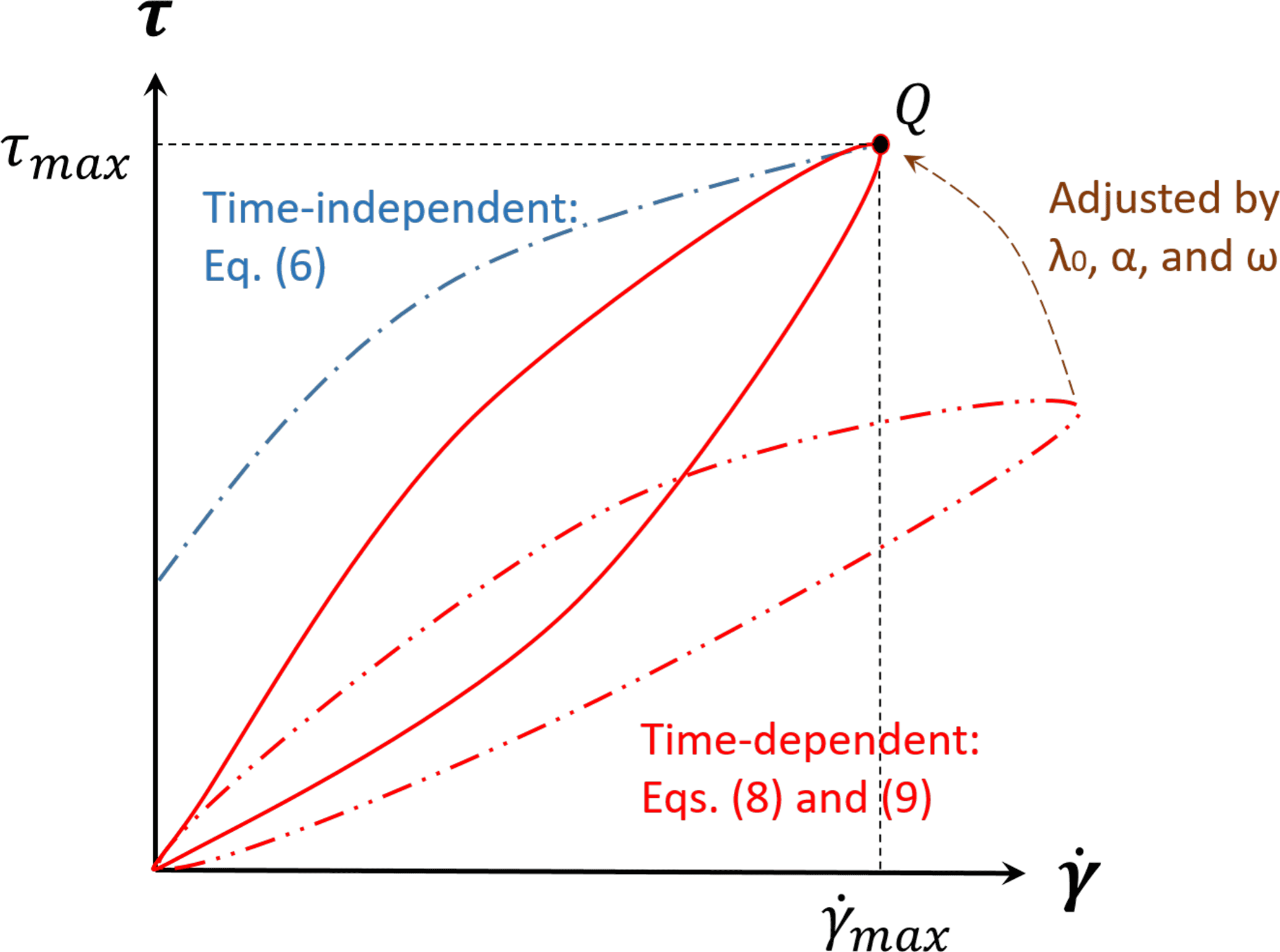
Figure 1Concept of a graphical method B for estimating a consistent set of ${\mathit{\lambda }}_{\mathrm{0}},\mathit{\alpha },and\mathit{\omega }$ parameters for the Coussot model.

Download

Some types of debris flow, such as avalanches, can be reasonably modeled as a single fluid with a free surface where dynamics of the overlying fluid (in this example, air) are neglected. In contrast, subaqueous debris flows are more likely to require coupled modeling between lighter overlying water (Newtonian fluid) and heavier non-Newtonian debris. It is also possible to imagine more complex configurations where simultaneous solution of multiple debris layers or perhaps debris, water, and air might be necessary. For general purposes, it is convenient to apply a multi-material level-set method so that any number of fluids with differing Newtonian and non-Newtonian properties can be considered. When only two fluids are considered, the multi-material level-set method corresponds to the general level-set method for two-phase flow. The level-set method has a long history in multi-phase fluids (Sussman et al., 1994; Chang et al., 1996; Sussman et al., 1998; Peng et al., 1999; Sussman and Fatemi, 1999; Bovet et al., 2010) and is based on using a ϕ_i distance (level set) function to represent the distance of the i material (or material phase) from an interface with another material (Osher and Fedkiw, 2001).

The multi-material level-set method herein follows Merriman et al. (1994) with the addition of high-order numerical schemes (Shu and Osher, 1989; Shi et al., 2002). The “level set” of the ith fluid is designated as ϕ_i:

where $i=\mathit{\{}\mathrm{1},\mathrm{2},\mathrm{\cdots },N_{\mathrm{m}}\mathit{\}}$, N_m is the number of materials, Γ_i is the interface of fluid i, and d is the distance from the interface. The density and viscosity at a computational node for the multiple-fluid system are evaluated from a combination of the individual fluid characteristics based on an approximate Heaviside function that provides a continuous transition over some ϵ distance on either side of an interface:

where the Heaviside function for fluid i is

where 2ϵ is therefore the finite thickness of the numerical interface between fluids.

The level-set initial condition is simply the distance from any grid point in the model to an initial set of interfaces, i.e., ϕ_i=d_i. Note that each point has a distance to each i interface. The level set is treated as a conservatively advected variable that evolves according to a simple non-diffusive transport equation (Osher and Fedkiw, 2001):

The above is coupled to a solution of momentum and continuity, Eqs. (2) and (3), to form a complete level-set solution for fluid flow. The continuous interface i at time t is located where ${\mathit{\varphi }}_i(\mathit{x},t)=\mathrm{0}$. In general, the i interface will be between the discrete grid points of the numerical solution, so it is found by multi-dimensional interpolation from the discrete ϕ_i values. After advancing the level set from ϕ(t) to ϕ(t+Δt), the values of the level set will no longer satisfy the eikonal condition of $\left|\mathrm{\nabla }{\mathit{\varphi }}_i\right|=\mathrm{1}$; that is, the level-set values on the grid cells obtained by solving Eq. (14) are no longer equidistant from the interface (i.e., the zero level set). It is known that if the level sets are naively evolved through time without satisfying the eikonal condition the Heaviside functions will become increasingly inaccurate (Sussman et al., 1994). This problem is addressed with “reinitialization”, which resets the ϕ(t+Δt) to satisfy the eikonal condition. The simplest approach to reinitialization is iterating an unsteady equation in pseudo-time to steady state such that the steady-state equation satisfies the eikonal condition (Sussman et al., 1998). Let $\widehat{\mathit{\varphi }}$ be an estimate of the reinitialized value for ϕ(t+Δt) in the equation

where 𝒯 is the pseudo-time, and S is the signed function as (Sussman et al., 1998)

The time-advanced set of ϕ(t+Δt) is the starting guess for $\widehat{\mathit{\varphi }}$, and the steady-state solution of $\widehat{\mathit{\varphi }}$ will satisfy $\left|\mathrm{\nabla }{\widehat{\mathit{\varphi }}}_i\right|=\mathrm{1}$ to numerical precision.

For the present work, the advection term in Eq. (14) is discretized with the fifth-order WENO scheme, and the time-derivative term is integrated by the third-order TVD Runge–Kutta method (Shu and Osher, 1989). For the reinitialization step of Eq. (15), the second-order ENO (essentially non-oscillatory) scheme (Sussman et al., 1998) and a smoothing approach (Peng et al., 1999) are used for the spatial discretization (further details are provided in Jeon, 2015).

A two-dimensional Poiseuille flow in a channel driven by a steady pressure gradient of $\partial p/\partial x$ provides a validation case for the non-Newtonian fluid solver. If gravity is considered negligible and the flow is approximated as symmetric about a centerline between two walls, then the analytical solution for the flow on one side of the centerline is (Papanastasiou, 1987)

where F is the distance from the center to a channel wall, y is the Cartesian axis normal to the flow direction with y=0 at the centerline of the flow between the two walls, τ₀ is the yield stress, and F_D is a length scale representing the relationship between yield stress and the pressure gradient:

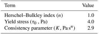
A convenient set of Bingham fluid parameters for the Poiseuille test cases can be extracted from the dip-coating study of Filali et al. (2013) as shown in Table 1. In the simulations, the distance from the centerline to a side wall is 0.05 m. Our model grid uses 320 cells in the flow direction and 32 cells in the cross-stream direction. A Neumann boundary condition is applied along the lower boundary of the simulation domain, so the simulation includes only the upper half-channel of this symmetric flow.

Using the Papanastasiou model of Eq. (6) to approximate a Herschel–Bulkley model of a Bingham fluid requires time-scale parameter m to provide smooth behavior across the yield-stress threshold. We tested values of $m=\left\{\mathrm{100},\mathrm{400}\right\}$ s. As shown in Fig. 2, the numerical results are in very good agreement with the analytical solutions for both values. For this simulation, the lower value of m=100 s is reasonable for a Papanastasiou model.

Table 1Bingham fluid Herschel–Bulkley model parameters used in Poiseuille flow test cases, from Filali et al. (2013).

Download Print Version | Download XLSX

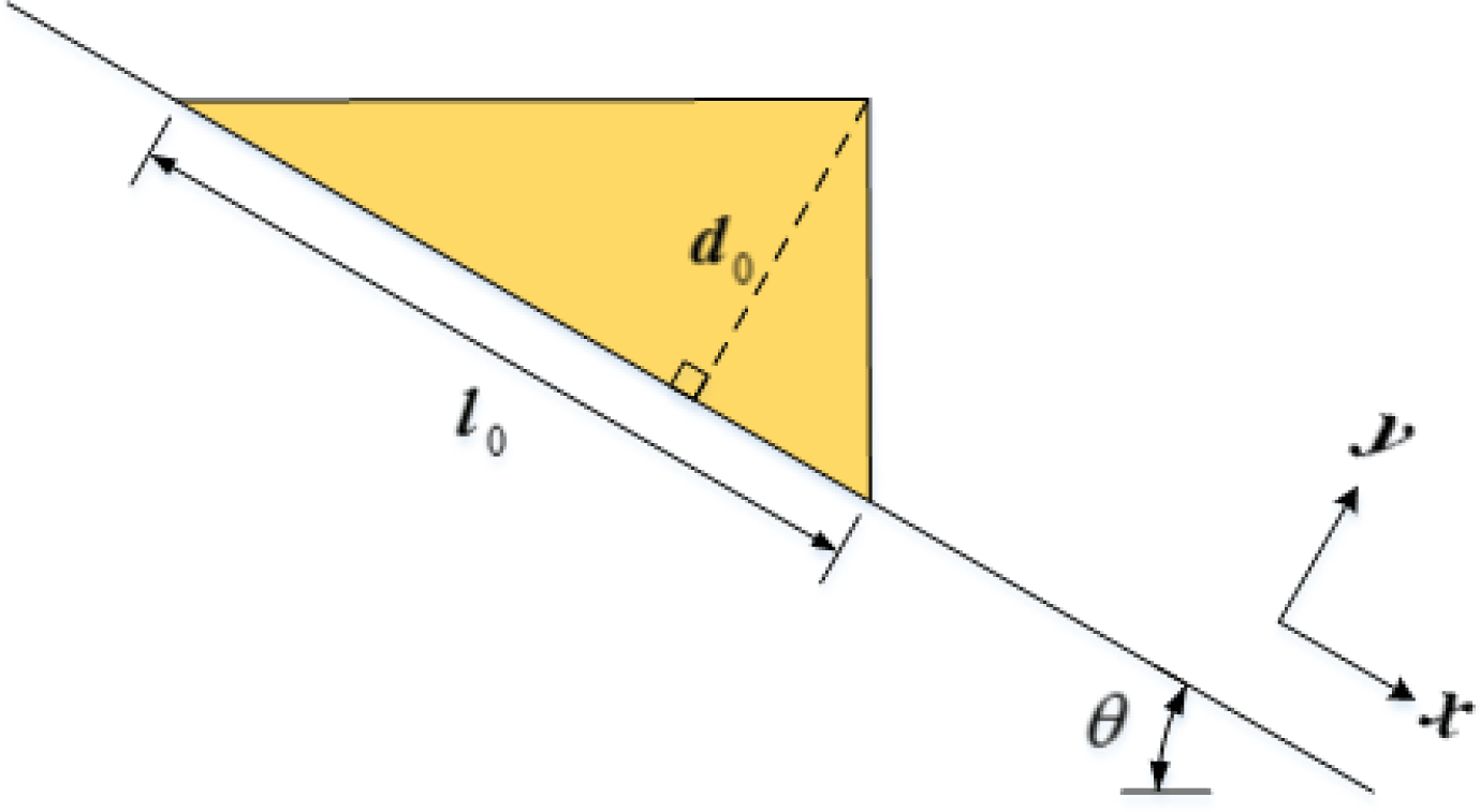
An avalanche is a granular flow of an initially solid field that is triggered from rest into a downslope flow. A thixotropic model of an avalanche as a fluid continuum can represent a rapid progression from local to global release of the initial structural jamming, λ₀. Chanson et al. (2006) developed dam-break experiments with a thixotropic fluid that provide reasonable facsimiles of avalanche flows if the timescale to remove the dam is smaller than the timescale for release of structural jamming. The initial conditions of the Chanson experiments are shown in Fig. 3 where θ, d₀, and l₀ represent the angle of a slope, the height of the initial avalanche that is normal to the slope, and the length of the avalanche along a slope, respectively. We modeled this same setup with our multi-material level-set solver.

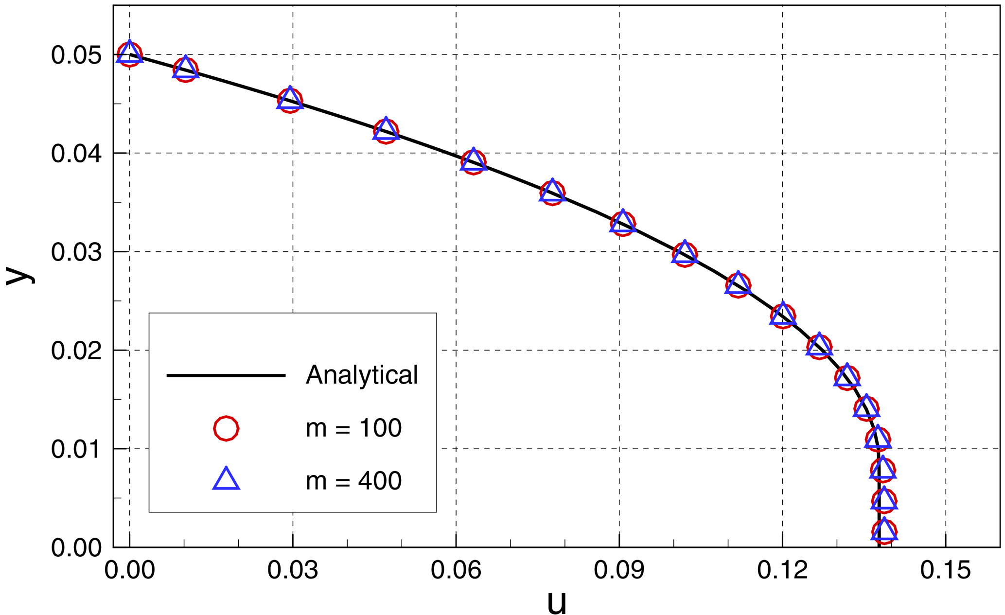
Figure 2Comparison of analytical and numerical solutions for steady-state fluid velocity for Poiseuille flow of a Bingham fluid.

Download

Figure 3Definition sketch for initial conditions of an avalanche along a slope.

Download

The Chanson experiments identified four thixotropic flow types that were functions of the relative effect of initial structural jamming. Weak jamming (i.e., small λ₀) characterizes type I, such that inertial effects dominate the downstream flow (highest Re) and the flow only ceases when it reaches the experiment outfall. It follows that type I is effectively a model of an avalanche that propagates until it is stopped by an obstacle or change in slope. Type II flows had intermediate initial jamming, which showed rapid initial flow followed by deceleration until “restructuralization”, which effectively stops the downstream progression. Type II is a model of an avalanche that dissipates itself on the slope. The type III flows, with the highest λ₀, have complicated behavior with separation into identifiable packets of mass (typically two, but sometimes more) with different velocities. Type IV behavior was the extremum of zero flow. Chanson reported 28 experiments in total, but data on wave front propagation were provided for only five experiments (Fig. 6 in Chanson et al., 2006) of type I and II behavior. We simulated three of these experiments that covered a wide range of characteristics and behaviors, as shown in Table 2. Note that Chanson et al. (2006) used τ_c2 to designate the critical shear stress during unloading (restructuralization), which we consider an approximation for the yield stress, τ₀, for a time-independent model.

We simulate the three cases of Table 2 with the time-independent Papanastasiou model of Eq. (6) and the time-dependent Coussot model of Eqs. (8) and (9). For a time-independent Bingham model, we use n=1 with K=η₀ from the Chanson experiments. The smoothing value of m=100 was selected based on the Poiseuille flow modeled in Sect. 6, above. For a time-independent Herschel–Bulkley model, we use the same K and m as the Bingham plastic model, but with n=1.1 as was used in the detailed technical report on the same experiments by Chanson et al. (2004). The time-dependent model requires specification of parameters $\left\{n,T_{\mathrm{0}},\mathit{\alpha },{\mathit{\eta }}_{\mathrm{0}},{\mathit{\lambda }}_{\mathrm{0}},\mathit{\omega }\right\}$ as discussed in Sect. 4. The Herschel–Bulkley index in the time-dependent model uses the same value (n=1.1) as the time-independent model. Two sets of values for $\left\{\mathit{\alpha },{\mathit{\lambda }}_{\mathrm{0}},\mathit{\omega }\right\}$ are determined by the two methods (A and B) outlined in Sect. 4, above. Method A uses Eq. (10), which requires a value for τ_c; herein this is taken as Chanson's critical loading stress (τ_c1 in Chanson et al., 2006) during the initial structural breakdown. Similarly, method B requires a τ_max for point Q in Fig. 1, which is also set to the critical loading stress.

Table 2Dimensions and data for thixotropic avalanche simulations corresponding with experiments by Chanson et al. (2006).

Download Print Version | Download XLSX

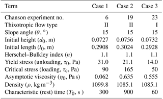
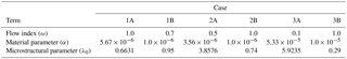
Table 3Parameters of the time-dependent fluid model for thixotropic avalanche simulations using method A and method B for setting values.

Download Print Version | Download XLSX

For all simulations, the no-slip wall condition is applied to the bottom wall, and the number of computational cells is 512 × 80. The computational domain is rotated so the x axis is along the sloping bed, which means that computational cell faces are either orthogonal or parallel to the slope. The gravitational constant (g = 9.81 m s⁻²) is divided into two components of (gsin θ, −gcos θ). The density and viscosity of air are 1.0 kg m⁻³ and 1.0 × 10⁻⁵ Pa s, respectively.

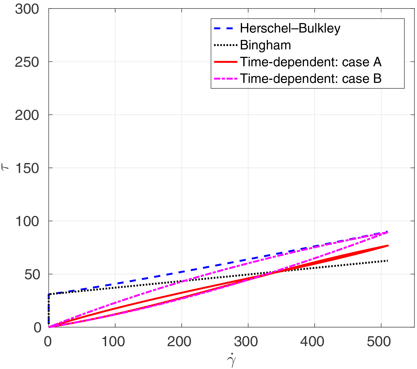
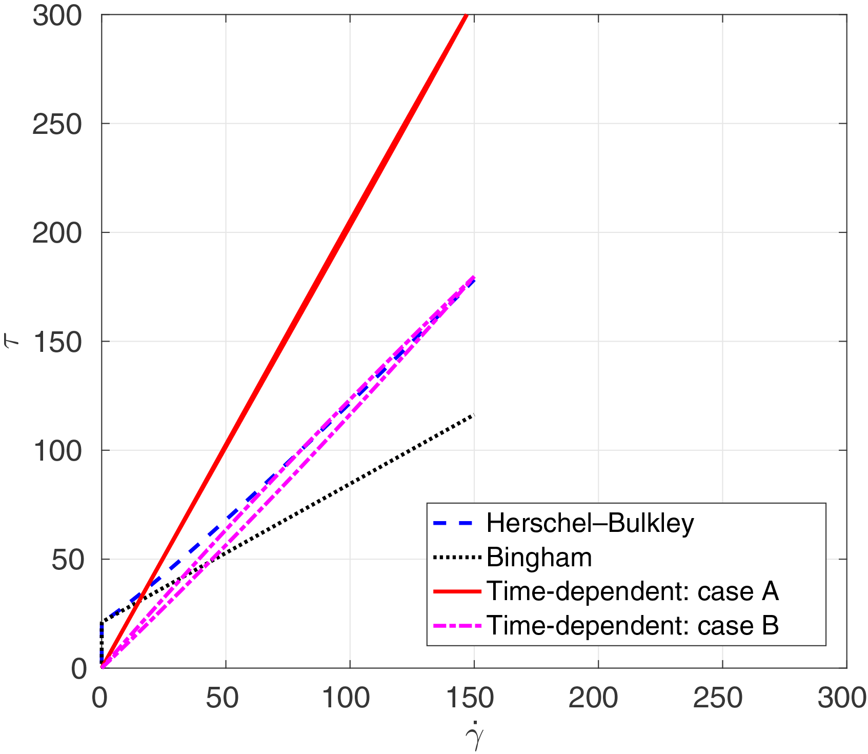
The analytical relationships between shear stress and rate of strain for the different viscosity models are presented in Figs. 4 through 6. In these figures, “Herschel–Bulkley” and “Bingham” lines are the results of Eq. (6) with n=1.1 and n=1.0, respectively. The “case A” and “case B” lines denote results of methods A and B from Sect. 4 for determining time-dependent parameters with Eqs. (8) and (9). The estimated parameters of λ₀, ω, and α by two methods that are used in these figures are shown in Table 3. These results illustrate the challenge of using method A (the critical stress relationship) for estimating λ₀. The numerical solutions of the Coussot model ordinary differential equation, Eq. (9), are obtained by the Runge–Kutta fourth-order method. The resulting time-dependent stress–strain relationship can be far from the time-independent relationship that is otherwise thought to be a reasonable model.

Figure 4Analytical stress–strain for thixotropic avalanche case 1: shear stress (Pa) and rate of strain (s⁻¹) with τ₀=31 Pa and τ_c=90 Pa. The τ axis is scaled for comparison with Figs. 5 and 6, while the $\dot{\mathit{\gamma }}$ axis has an individual scale for clarity.

Download

Figure 5Analytical stress–strain for thixotropic avalanche case 2: shear stress (Pa) and rate of strain (s⁻¹) with τ₀=21.1 Pa and τ_c=165 Pa. The τ axis is scaled for comparison with Figs. 4 and 6, while the $\dot{\mathit{\gamma }}$ axis has an individual scale for clarity.

Download

Propagation of the fluid wave front provides a simple means of directly comparing the temporal and spatial evolution of the model and experiments. To facilitate comparisons across experimental scales, the non-dimensionalized front location and simulation time after gate opening are $x^{\ast }=x/d_{\mathrm{0}}$ and $t^{\ast }=t\sqrt{g/d_{\mathrm{0}}}$, respectively. A simple theoretical estimate for the wave front propagation suitable for short timescales was derived from equations of motion as Eq. (26) in Chanson et al. (2006), repeated here as

The simulation, experiment, and theory results are shown in Figs. 7, 8, and 9 for cases 1, 2, and 3 of Table 2, respectively. The dashed line represents the theoretical solution for propagating the front of Eq. (18).

Figure 6Analytical stress–strain for thixotropic avalanche case 3: shear stress (Pa) and rate of strain (s⁻¹) with τ₀=14 Pa and τ_c=50 Pa. The τ axis is scaled for comparison with Figs. 4 and 5, while the $\dot{\mathit{\gamma }}$ axis has an individual scale for clarity.

Download

The most striking feature in the results is that the simulations for cases 2 and 3 (smaller τ₀) are relatively similar for all the models, whereas the time-independent models (Bingham and Herschel–Bulkley) completely fail for case 1 (larger τ₀) even though the time-dependent models continue to perform reasonably well. The failure appears to be due to an inability of the time-independent models in case 1 to develop sufficient strain to move out of the $\mathit{\eta }=K{\dot{\mathit{\gamma }}}^{n-\mathrm{1}}+m{\mathit{\tau }}_{\mathrm{0}}$ regime that governs viscosity below the yield stress in Eq. (6). In contrast, the microstructural aging process that is inherent in Eqs. (8) and (9) allows the time-dependent models in case 1 to develop reasonable flow conditions despite the higher τ₀. No doubt the time-independent models could be made to perform better in case 1 by further manipulation of the model coefficients; however, our approach was to use coefficients that could be set a priori based on data from the experiments and a plausible m value from Sect. 6.

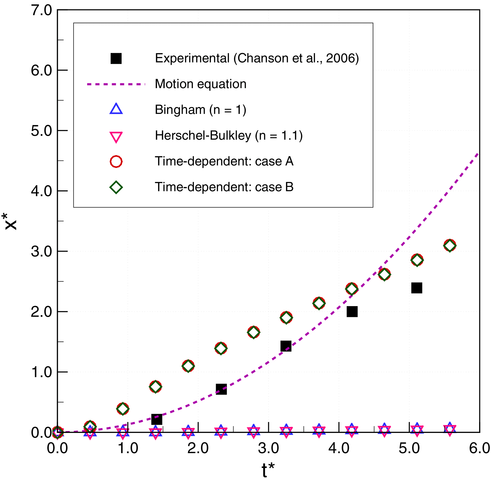
Figure 7Thixotropic avalanche case 1: comparison of numerical results and experimental data for non-dimensional front displacement (x^∗) as a function of non-dimensional simulation time (t^∗).

Download

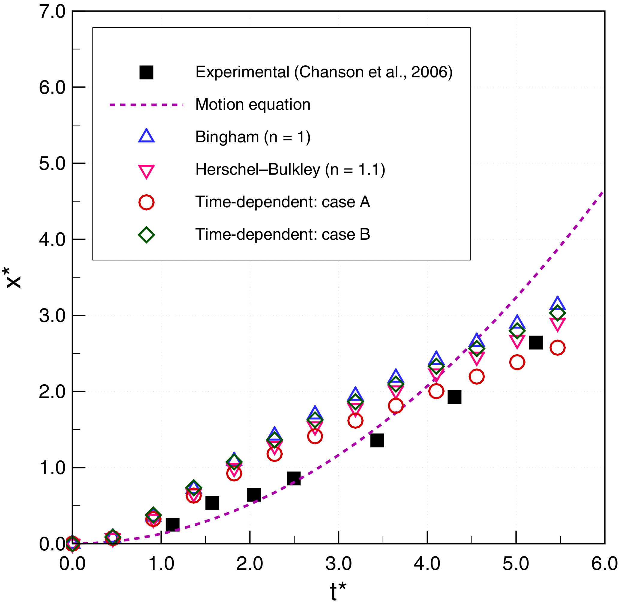
Figure 8Thixotropic avalanche case 2: comparison of numerical results and experimental data for non-dimensional front displacement (x^∗) as a function of non-dimensional simulation time (t^∗).

Download

Figure 9Thixotropic avalanche case 3: comparison of numerical results and experimental data for non-dimensional front displacement (x^∗) as a function of non-dimensional simulation time (t^∗).

Download

We observe that the simplified theoretical front prediction from Eq. (18), the dashed line in the figures, is a good representation of Chanson's type II flows (case 1 and case 2) up until $t^{\ast }\sim \mathrm{3}$, but it diverges rapidly thereafter. Our 2-D simulations consistently overpredict the experimental front propagation in the early stages for cases 1 and 2 but show better agreement with experiments than the simplified theory for $t^{\ast }>\mathrm{4}$. However, for case 3 (type I flow), the simplified theory is relatively poor, while the 2-D simulations have good agreement up until $t^{\ast }\sim \mathrm{3}$ and then show significant underprediction of the experiments. As noted by Chanson et al. (2006), the case 3 (type I) experiments are at higher Reynolds numbers that, although theoretically laminar, may be transitioning to weakly turbulent. Because the simplified theory of Eq. (18) is derived by neglecting inertia, it is not surprising that its performance degrades with increasing Reynolds number.

Although the simulations results have reasonable global agreement with experiments, on closer examination it can be seen that the 2-D simulations predict a front movement that is initially too rapid in type II flows (cases 1 and 2) and at longer times is too slow for type I flows (case 3). The challenge, of course, is that the model error is integrative: if λ is wrong at a given time, then the dλ∕dt will be wrong as well and the frontal position error will accumulate. Thus, an important issue for the time-dependent model appears to be selecting the appropriate values of $\left\{{\mathit{\lambda }}_{\mathrm{0}},\mathit{\alpha },\mathit{\omega }\right\}$ that are consistent with experimentally determined values of $\left\{{\mathit{\eta }}_{\mathrm{0}},{\mathit{\tau }}_{\mathrm{0}},{\mathit{\tau }}_{\mathrm{c}},n,T_{\mathrm{0}}\right\}$. Although the more parsimonious time-independent model (with fewer parameters) performs reasonably well for our cases 2 and 3, it performs poorly in case 1 and so should only be used with caution and careful calibration.

The above observations lead to a conclusion that the accelerative behaviors in the simulations and experiments are not well matched. The problem is shown most clearly in Fig. 7 for case 1, where the experiments initially follow the acceleration implied by Eq. (18) but diverge with an inflection point and deceleration occurring somewhere near $t^{\ast }\sim \mathrm{4}$. In contrast, the models initially show a more rapid acceleration and an inflection point to deceleration at $t^{\ast }\sim \mathrm{1}$. Interestingly, the simulated front locations in cases 1 and 2 are not unreasonable predictions for $t^{\ast }>\mathrm{4}$, but they get there along slightly different paths than the experiments. The case 3 (type I) models show different behaviors: they perform quite well for $t^{\ast }\le \mathrm{3}$ and then show deceleration at the same time as the experiment appears to be accelerating. Unfortunately, the experiments of Chanson et al. (2006) did not extend beyond $t^{\ast }\sim \mathrm{6.5}$, so it is impossible to know whether the experiments are showing an inflection point to deceleration at $t^{\ast }\sim \mathrm{5}$, but it seems likely given the results of the case 1 and 2 studies. If there is an inflection point for case 3, then it would appear that the consistent problem with the models is getting the correct transition from frontal acceleration to deceleration. To date, our experiments have not shown that we can significantly alter the model acceleration inflection points by altering parameters, which may indicate that there is a need to further consider the fundamental forms of the Coussot and Papanastasiou models when used for thixotropic flows. An alternative explanation may be that there are three-dimensional controls on the front propagation in the experiment that cannot be represented in the present 2-D model.

In general, subaqueous debris flows are heterogenous gravity flows where the interaction of the overlying water with the downslope flow of the debris has a significant effect on momentum. Such flows are expected to be qualitatively similar to the subaqueous mud flow examined in the laboratory by Haza et al. (2013). We conducted simulations matching the Haza et al. (2013) experimental cases with the largest density difference between the water and mud. These conditions provide the largest effective negative buoyancy for the debris and minimize effect of turbidity. The selected cases are 35 and 30 % KCC (kaolin clay content). The schematic design is shown in Fig. 10, with dimensions provided in Table 4. The gravitational constant for all simulations is g=9.81 m s⁻².

The simulation uses 340 × 100 rectangular cells. The no-slip wall boundary condition is applied to the bottom boundary. The computational domain is rotated so the x axis is parallel to the slope, which allows the bottom to be represented as a straight surface without using cut grid cells or unstructured grids. This rotation also provides convenience in measuring the variables normal to the slope (e.g., front distance and water/mud thicknesses at the front.) These simulations include three fluids: mud, water, and air. The density of mud for each case is shown in Table 6, and the densities of water and air are 1000.0 and 1.0 kg m⁻³, respectively.

Figure 10Submarine landslide.

Download

Figure 11Subaqueous debris case 1: shear stress (Pa) and rate of strain (s⁻¹).

Download

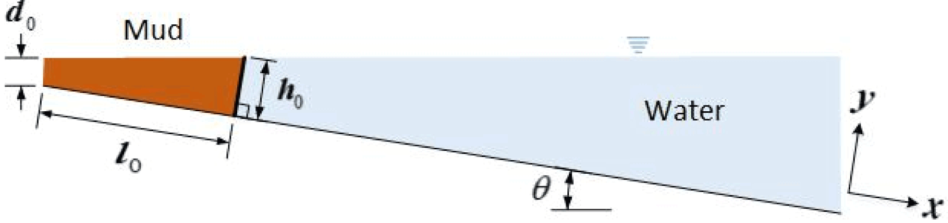
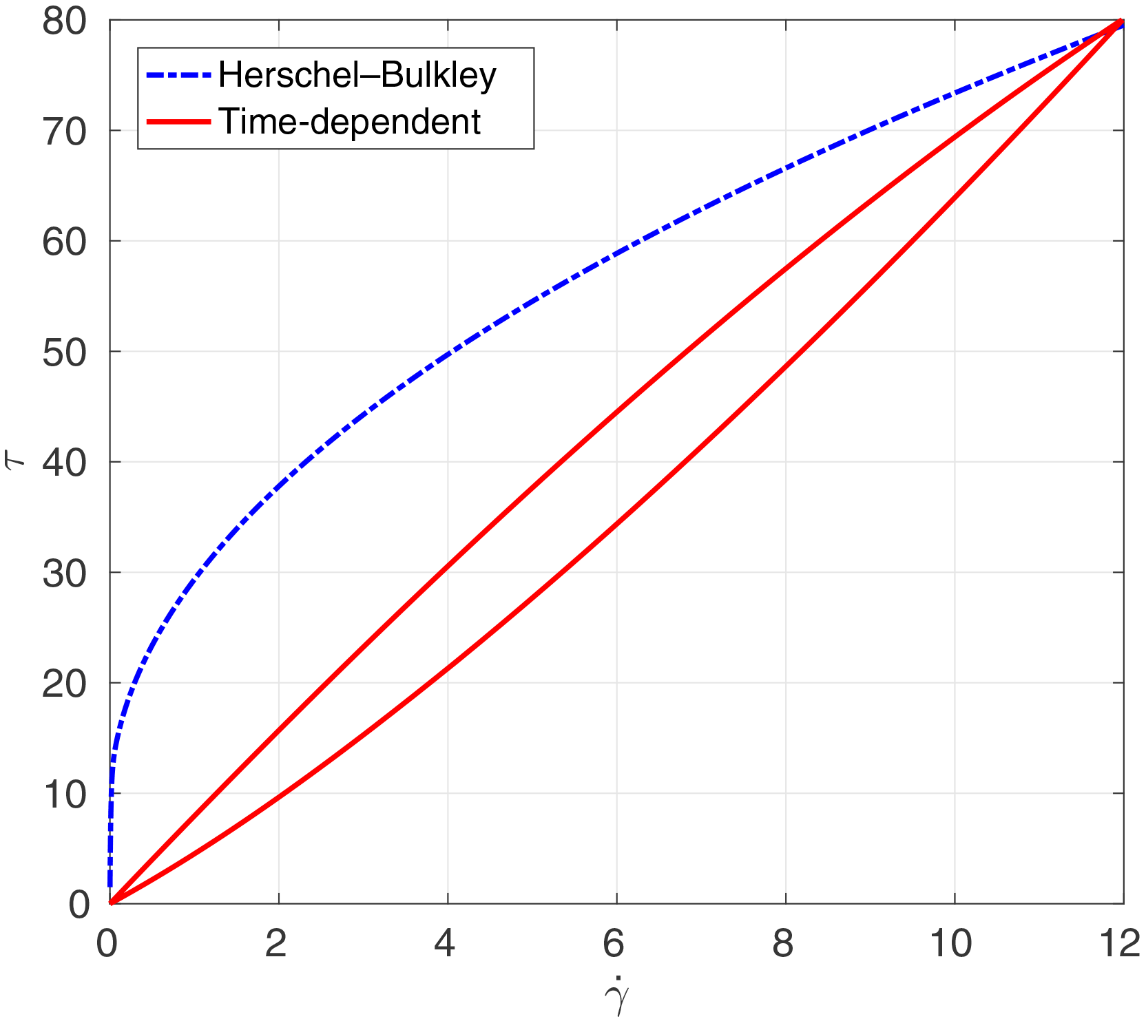
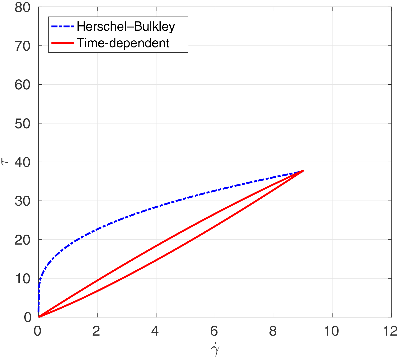
Figure 12Subaqueous debris case 2: shear stress (Pa) and rate of strain (s⁻¹). Axis scalings are identical to Fig. 11 for comparison purposes.

Download

Figure 13Run-out and head flow.

Download

The parameters for the time-independent fluid model from Haza et al. (2013) are shown in Table 5. For all simulations, m=100 for the exponential smoothing parameter is used based on results from Sect. 6, above. The parameters for the time-dependent fluid model are estimated from method B in Sect. 4 and are shown in Table 6. The experiments did not report a rest time, so T₀ was set at a small positive value that provided a reasonable match to the experiments. The analytical relationships between the shear stress and the rate of strain for the time-independent and the time-dependent fluid models are shown in Fig. 11 for case 1 and Fig. 12 for case 2.

Table 4Dimensions for simulations to match experiments by Haza et al. (2013).

Download Print Version | Download XLSX

Table 5Parameters of the time-independent fluid model.

Download Print Version | Download XLSX

Table 6Parameters of the time-dependent fluid model.

Download Print Version | Download XLSX

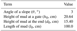
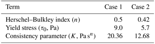
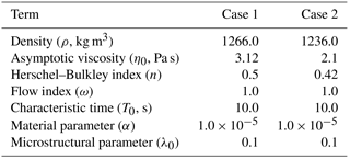
Figure 13 provides a reference for measurements used to compare the model and experiments. These include the height of head flow (H), the water depth at the front of head flow (D), the run-out distance from the initial position (L), and the flow-front velocity (U). Figure 14 shows evolution of the zero level sets for water (ϕ₂), which provides the continuous line separating the water from both the debris and the air. Figures 15 and 16 show the evolution of the run-out distance (L) for case 1 and case 2, respectively. It can be seen that both time-independent and time-dependent models are reasonable approximations of the limited experimental data. Both types of models appear to underestimate the initial run-out and slightly overestimate later times.

Figure 14Profiles of debris and water (ϕ₂: water).

Download

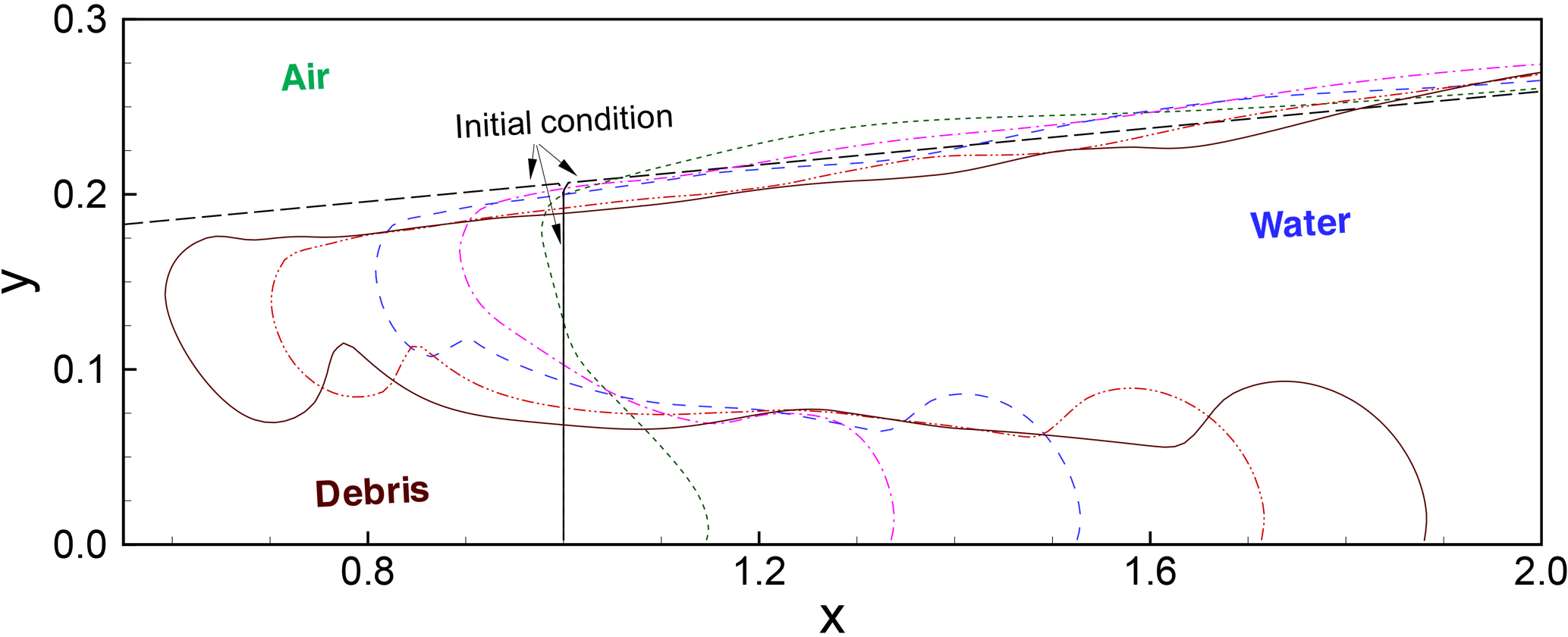
Figure 15Subaqueous debris case 1: run-out distance (L, m) as a function of simulation time (t, s).

Download

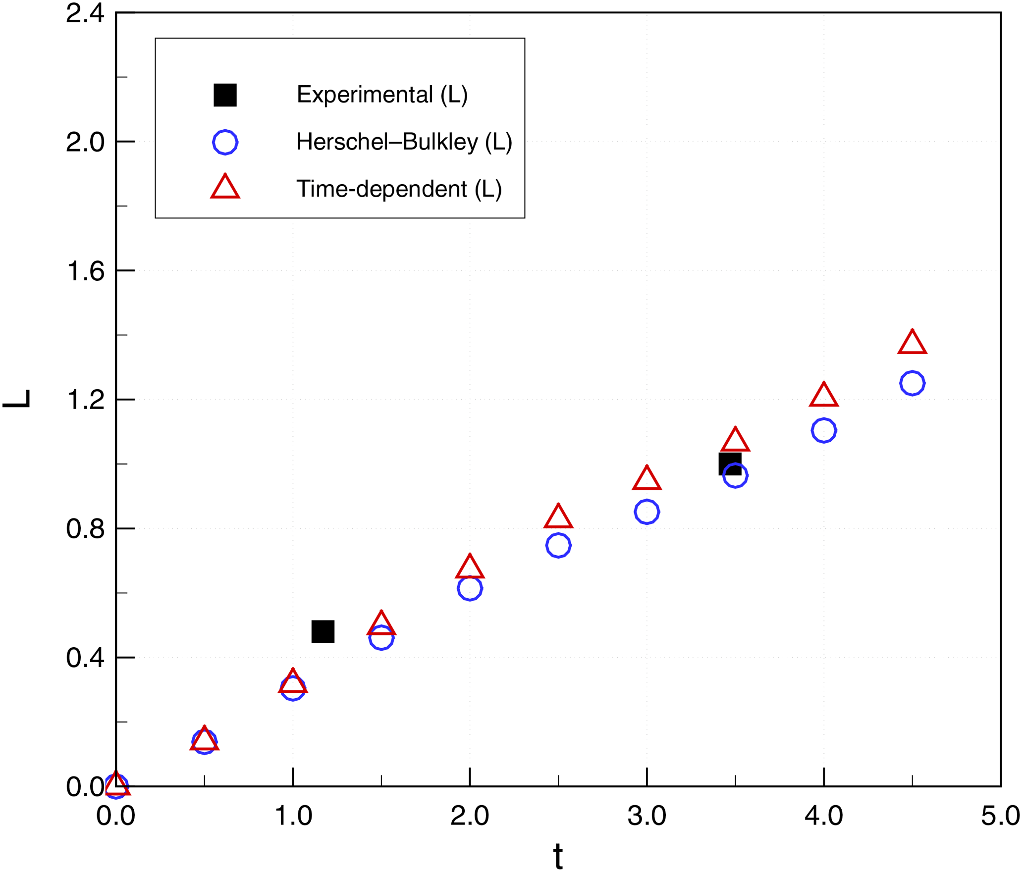
Figure 16Subaqueous debris case 2: run-out distance (L, m) as a function of simulation time (t, s).

Download

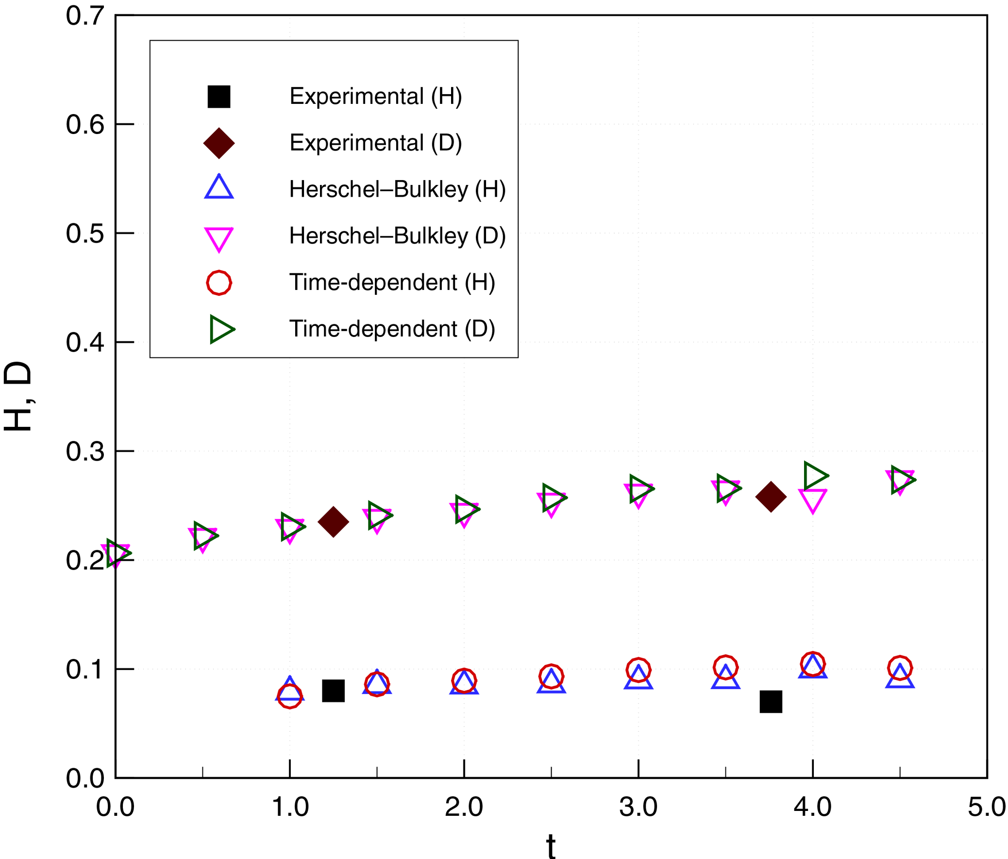
Figure 17Subaqueous debris case 1: height of head flow (H, m) and water depth (D, m) as a function of simulation time (t, s).

Download

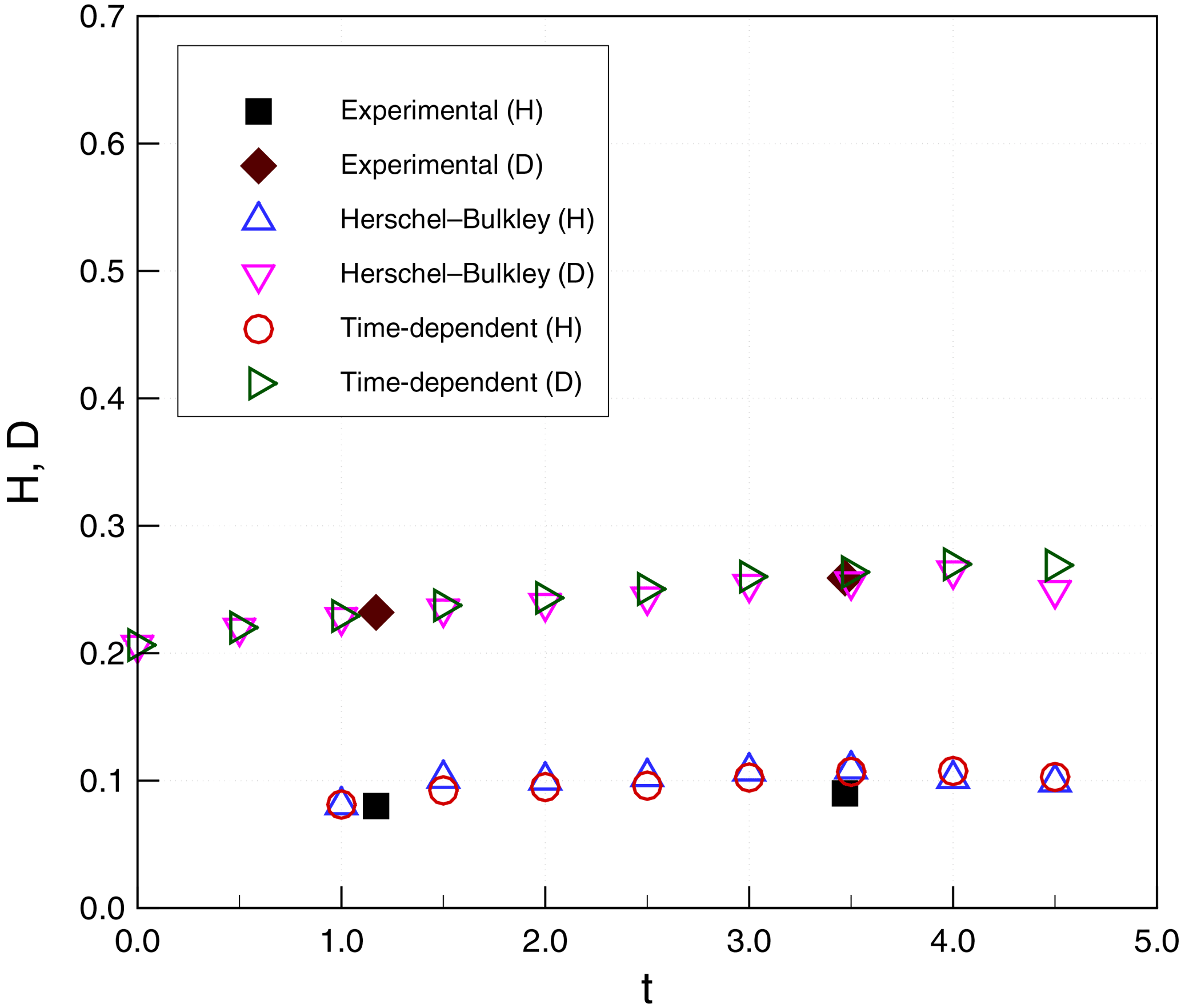
Figure 18Subaqueous debris case 2: height of head flow (H, m) and water depth (D, m) as a function of simulation time (t, s).

Download

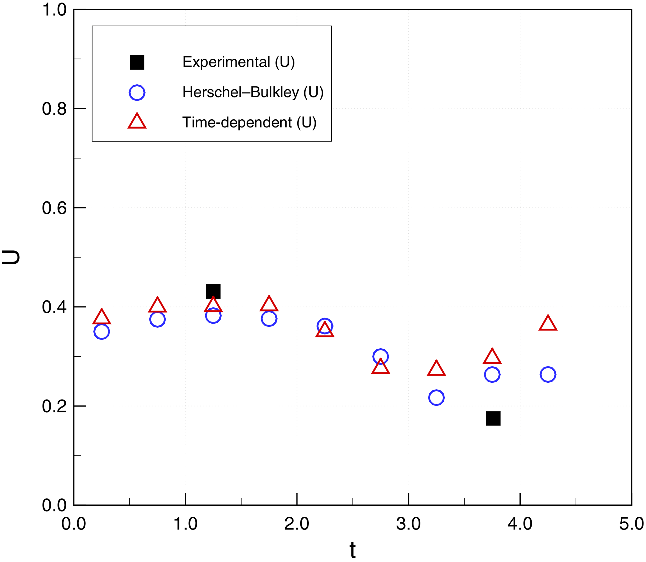
Figure 19Subaqueous debris case 1: flow-front velocity (U, m s⁻¹) as a function of simulation time (t, s).

Download

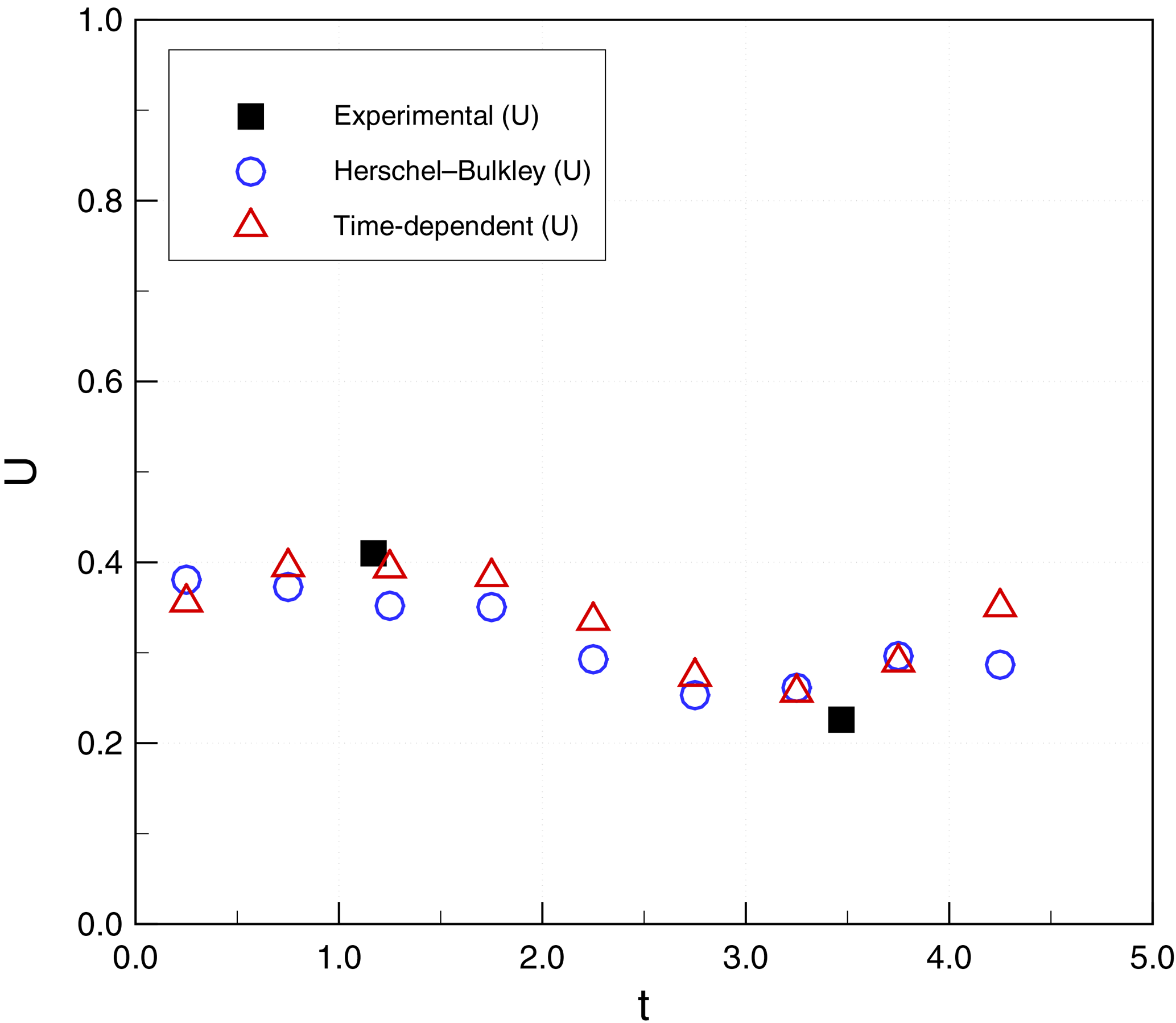
Figure 20Subaqueous debris case 2: flow-front velocity (U, m s⁻¹) as a function of simulation time (t, s).

Download

Figures 17 and 18 show a comparison of H and D for simulations and experiments. Again, within the limited availability of experimental data, both time-independent and time-dependent models provide reasonable agreement. Figures 19 and 20 show similar agreement for the front velocities, although the experimental data are insufficient to validate the wave-like oscillation of the velocity in the simulations.

These results indicate the multi-material level-set model is capable of representing the key features in a subaqueous debris flow. For this flow, the use of the simpler time-independent viscosity model seems justified, although this is likely a function of the experimental conditions. An important limitation of the tested subaqueous debris flows is that they do not have the restructuralization in the downstream flow or the strongly jammed initial structure seen in the experiments of Chanson et al. (2006)

The experimental data in the figures can be found in Chanson et al. (2006) and Haza et al. (2013). The simulation data can be obtained from the corresponding author (Chan-Hoo Jeon).

The authors declare that they have no conflict of interest.