Scale and spatial distribution assessment of rainfall-induced landslides in a catchment with mountain roads

Tseng, Chih-Ming; Chen, Yie-Ruey; Wu, Szu-Mi

doi:https://doi.org/10.5194/nhess-18-687-2018

Articles | Volume 18, issue 2

https://doi.org/10.5194/nhess-18-687-2018

Special issue:

Landslide–transport network interactions

https://doi.org/10.5194/nhess-18-687-2018

Articles | Volume 18, issue 2

Research article

02 Mar 2018

Research article |

| 02 Mar 2018

Scale and spatial distribution assessment of rainfall-induced landslides in a catchment with mountain roads

Chih-Ming Tseng, Yie-Ruey Chen, and Szu-Mi Wu

Abstract

This study focused on landslides in a catchment with mountain roads that were caused by Nanmadol (2011) and Kong-rey (2013) typhoons. Image interpretation techniques were employed to for satellite images captured before and after the typhoons to derive the surface changes. A multivariate hazard evaluation method was adopted to establish a landslide susceptibility assessment model. The evaluation of landslide locations and relationship between landslide and predisposing factors is preparatory for assessing and mapping landslide susceptibility. The results can serve as a reference for preventing and mitigating slope disasters on mountain roads.

Download & links

Article (PDF, 4659 KB)

How to cite

How to cite.

Dates

Received: 14 Jul 2017 – Discussion started: 04 Oct 2017 – Revised: 27 Dec 2017 – Accepted: 22 Jan 2018 – Published: 02 Mar 2018

1 Introduction

Taiwan is an island with three quarters of its land area consisting of slope land that is 100 $m a . s . l .$ , or less but has an average gradient of 5 % above (SWCB, 2017). Much of this sloped land has a steep gradient and fragile geological formations. Taiwan is hit by an average of 3.4 typhoons every year during the years 1911 to 2016 (Central Weather Bureau, 2017). In addition, average annual rainfall reaches 2502 mm in the years 1949 to 2009 (Water Resources Agency, 2017). Typhoons usually occur between July and October, and 70–90 % of the annual rainfall is composed of heavy rain directly related to typhoons (SWCB, 2017). Concentrated rainfall causes heavy landslides and debris flows every year (Dadson et al., 2004). The threat of disaster currently influences industrial and economic development and the road networks in endangered areas, thus establishing disaster evaluation mechanisms is imperative.

Landslide susceptibility can be evaluated by analysing the relationships between landslides and various factors that are responsible for the occurrence of landslides (Brabb, 1984; Guzzetti et al., 1999, 2005). In general, the factors that affect landslides include predisposing factors (e.g. geology, topography, and hydrology) and triggering factors (e.g. rainfall, earthquakes, and anthropogenic factors) (Chen et al., 2013a, b; Chue et al., 2015). Geological factors include lithological factors, structural conditions, and soil thickness; topographical factors include slope, aspect, and elevation; and anthropogenic factors include deforestation, road construction, land development, mining, and alterations of surface vegetation (Chen et al., 2013a, b; Chue et al., 2015). The method used to assess landslide susceptibility can be divided into qualitative and quantitative. Qualitative methods are based completely on field observations and an expert's prior knowledge of the study area (Stevenson, 1977; Anbalagan, 1992; Gupta and Anbalagan, 1997). Some qualitative approaches incorporate ranking and weighting, and become semi-quantitative (Ayalew and Yamagishi, 2005). For example the analytic hierarchy process (AHP) (Saaty, 1980; Barredo et al., 2000; Yoshimatsu and Abe, 2006; Kamp et al., 2008; Yalcin, 2008; Kayastha et al., 2013; Zhang et al., 2016) and the weighted linear combination (WLC) (Jiang and Eastman, 2000; Ayalew et al., 2005; Akgün et al., 2008). Quantitative methods apply mathematical models to assess the probability of landslide occurrence, and thus define hazard zones on a continuous scale (Guzzetti et al., 1999). Quantitative methods developed to detect the areas prone to landslide can be divided mainly into two categories: deterministic approach and statistical approach. The deterministic approach is based on the physical laws driving landslides (Okimura and Kawatani, 1987; Hammond et al., 1992; Montgomery and Dietrich, 1994; Wu and Sidle, 1995; Gökceoglu and Aksoy, 1996; Pack et al., 1999; Iverson, 2000; Guimarães et al., 2003; Xie et al., 2004) and are generally more applicable when the underground conditions are relatively homogeneous and the landslides are mainly slope dominated. The statistical approach is based on the relationships between the affecting factors and past and present landslide distribution (Van Westen et al., 2008). Statistical methods analyse the relation between predisposing factors affecting the landslide which include bivariate statistical models (Van Westen et al., 2003; Süzen and Doyuran, 2004; Thiery et al., 2007; Bai et al., 2009; Constantin et al., 2011; Yilmaz et al., 2012), multivariate statistical approaches as discriminant analysis (Baeza and Corominas, 2001; Carrara et al., 2003, 2008; Pellicani et al., 2014), and linear and logistic regression (Dai and Lee, 2002; Ohlmacher and Davis, 2003; Ayalew and Yamagishi, 2005; Yesilnacar and Topal, 2005; Greco et al., 2007; Carrara et al., 2008; Lee et al., 2008; Pellicani et al., 2014), as well as non-linear methods such as artificial neural networks (ANN) (Lee et al., 2004; Yesilnacar and Topal, 2005; Kanungo et al., 2006; Wang and Sassa, 2006; Li et al., 2012) and multivariate hazard evaluation method (MHEM) (Su et al., 1998; Lin et al., 2009). The MHEM is a non-linear mathematical model that presents an instability index to indicate landslide susceptibility (Lin et al., 2009). In addition, in some studies, landslide susceptibility analyses have focused on man-made facilities such as roads and railroads and have examined the landslide susceptibility of the surrounding environments (Das et al., 2010, 2012; Pantelidis, 2011; Devkota et al., 2013; Martinović et al., 2016; Pellicani et al., 2016, 2017). The aforementioned studies on the landslide susceptibility of areas surrounding man-made facilities have not investigated characteristics such as the location and scale (area) of landslides occurring in upper or lower slopes, and these thus constitute one of the objectives of the present study.

Technological progress has provided various advanced tools and techniques for land use monitoring. In recent years, aerial photos or satellite images have been commonly used in post-disaster interpretations and assessments of landslide damage on large-area slopes (Erbek et al., 2004; Lillesand et al., 2004; Nikolakopoulos et al., 2005; Lin et al., 2005; Chen et al., 2009; Otukei and Blaschke, 2010; Chen et al., 2013a). Satellite images offer the advantages of short data acquisition cycles, swift understanding of surface changes, large data ranges, and being low cost, particularly for mountainous and inaccessible areas. With the assistance of computer analysis and geographic information system (GIS) platforms, researchers can quickly determine land cover conditions. Thus, satellite images are suitable for investigating large areas and monitoring temporal changes in land use (Liu et al., 2001). Satellites can capture images of the same area multiple times within a short period. Studies have indicated that land surface change detection is the process of exploring the differences between images captured at different times (Liu et al., 2001; Chadwick et al., 2005; Chen et al., 2009; Chue et al., 2015). With multispectral satellite images, land surface interpretations involve comparisons of multitemporal images that are completely geometrically aligned.

We selected part of the catchment area of Laonung River which include Provincial Highway 20 in southern Taiwan as our study area. Regarding time, we focused on periods before and after landslides that occurred in the study area as a result of Typhoon Nanmadol (2011) and Typhoon Kong-rey (2013). We applied the maximum likelihood method to interpret and categorize high-resolution satellite images, thereby determining the land surface changes and landslides in the study area before and after the rainfall events. By using a GIS platform, we constructed a database of the rainfall and natural environment factors. Subsequently, we developed a landslide susceptibility assessment model by using the MHEM. The model performance was then verified by historical landslides. In addition, we extracted the locations of landslide areas to explore the relationship between the natural environment and the spatial distribution of the scale of these areas.

2 Methodology

2.1 Maximum likelihood

The maximum likelihood classifier is a supervised classification method (SCM). SCMs include three processing stages: training data sampling, classification, and output. The underlying principle of supervised classification is the use of spectral pattern recognition and actual ground surface data to determine the types of data required and subsequently select a training site, which has a unique set of spectral patterns. To accurately estimate the various spectral conditions, the spectral patterns of the same type of feature are combined into a coincident spectral plot before the class of the training site is selected. Once training has been completed, the entire image is classified based on the spectral distribution characteristics of the training site by using statistical theory for automatic interpretation (Lillesand et al., 2004).

To facilitate the calculation of probability in the classification of unknown pixels, the maximum likelihood method assumes a normal distribution in the various classes of data. Under this assumption, the data distribution can be expressed using covariance matrices and mean vectors, both of which are used to calculate the probability of a pixel being assigned to a land cover class. In other words, the probability of X appearing in class i is calculated using Eq. (1), and the highest probability is used to determine the feature of each pixel (Lillesand et al., 2004).

\begin{array}{l} p (X | C_{i}) = \\ (1) & {(2 π)}^{d / 2} {|\sum_{i}|}^{- 1 / 2} \exp [- \frac{1}{2} {(X - μ_{i})}^{T} \sum_{i}^{- 1} (X - μ_{i})] \\ X = [\begin{array}{c} X_{1} \\ X_{2} \\ ⋮ \\ X_{d} \end{array}] μ_{i} = [\begin{array}{c} μ_{1 i} \\ μ_{2 i} \\ ⋮ \\ μ_{di} \end{array}] \sum_{i} = [\begin{array}{cccc} S_{11} & S_{12} & \dots & S_{1 d} \\ S_{21} & S_{22} & \dots & S_{2 d} \\ ⋮ & ⋮ & ⋱ & ⋮ \\ S_{d 1} & S_{d 2} & \dots & S_{dd} \end{array}] \end{array}

In this equation, d denotes the number of features, X denotes a sample expressed using features and has d dimensions, p(X|C_i) denotes the probability that X originates from class i, Σ_i denotes the covariance matrix of class i, $Σ_{i}^{- 1}$ denotes the inverse matrix of Σ_i, $| Σ_{i} |$ denotes the determinant of Σ_i, μ_i denotes the mean vector of classification i, (X−μ_i)^T denotes the transpose matrix of (X−μ_i), and S_ij denotes the covariance of classes i and j.

During classification, the maximum value of the probability density functions of sample X in each class is used to determine which class the sample belongs to. The maximum likelihood classification decision is shown in Eq. (2).

X \in C_{m}, m \subset \{1, 2, \dots, k\}

\begin{matrix} (2) & p (X| C_{m}) = max \{p (X | C_{j}), j = 1, 2, \dots k\}, \end{matrix}

in which k denotes the number of classes. The question regarding classification is how to effectively separate the classes in the feature space, or in other words, how to divide the feature space. Maximum likelihood is a common approach that offers fairly good classification accuracy (Bruzzone and Prieto, 2001; Chen et al., 2004). Thus, we adopted maximum likelihood to interpret and classify the satellite images.

2.2 Accuracy assessment

This study employed the aforementioned maximum likelihood method to classify satellite images. To determine whether the accuracy of image classification was acceptable, we adopted an error matrix to test for accuracy. An error matrix is a square matrix that presents error conditions in the relationship between ground surface classification results and reference data (Verbyla, 1995). It contains an equal number of columns and rows, and the number is determined by the number of classes. For example, Table 1 contains four classes. The columns show the reference data, and the rows show the classification results. The various elements in the table indicate the quantity of data corresponding to each combination of classes.

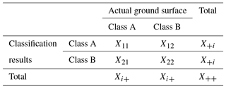
Table 1Relationship table of error matrix (Verbyla, 1995).

Download Print Version | Download XLSX

In the Table 1, X₁₂ represents the amount of data that were interpreted as Class A but actually belong to Class B, whereas X₂₁ indicates the amount of data that were interpreted as Class B but actually belong to Class A. X₁₁ and X₂₂ represent the amount of data accurately classified as Class A and Class B. An error matrix is generally used to check the quality of classification results in statistics (Congalton, 1991; Verbyla, 1995). In the present study, we evaluated the accuracy of the classification results based on the overall accuracy and kappa value (Cohen, 1960), which is the coefficient of agreement derived from the relationship between the classification results and training data. These two parameters are explained as follows.

2.2.1 Overall accuracy (OA)

OA is the simplest method of overall description. For all classes, OA represents the probability that any given point in the area will be classified correctly.

\begin{matrix} (3) & OA = [\frac{1}{N} \sum_{i = 1}^{n} X_{ii}] \times 100 % \end{matrix}

In Eq. (3), N denotes the total number of classifications, n denotes the total number of rows in the matrix, and X_ii is the number of correctly classified checkpoints.

2.2.2 Kappa coefficient

The kappa ( $\hat{K}$ ) coefficient indicates the degree of agreement between the classification results and reference values and shows the percentage reduction in the errors of a classification process compared with the errors of a completely random classification process. Generally, the kappa coefficient ranges from 0 to 1, and a greater value indicates a higher degree of agreement between the two sets of results, as shown in Eq. (4):

\begin{matrix} (4) & \hat{K} = \frac{N \sum_{i = 1}^{n} X_{ii} - \sum_{i = 1}^{n} (X_{i +} \times X_{+ i})}{N^{2} - \sum_{i = 1}^{n} (X_{i +} \times X_{+ i})} \times 100 %, \end{matrix}

in which X_i+ is the total number of pixels for a given class on the actual ground surface and X_+i is the number of pixels in that class. As reported by Landis and Koch (1977), a kappa coefficient greater than 0.8 signifies a high degree of accuracy, whereas a coefficient between 0.4 and 0.8 or less than 0.4 indicates moderate or poor accuracy.

2.3 Rainfall analysis method

In previous studies regarding the influence of rainfall on landslides, rainfall intensity and accumulated rainfall have been most commonly used as predisposing factors of landslides (Giannecchini, 2006; Chang et al., 2007; Giannecchini et al., 2012; Ali et al., 2014). Therefore, we adopted effective accumulated rainfall and intensity of rolling rainfall as rainfall indices and predisposing factors of landslides in the present study. These two indices are explained as follows.

2.3.1 Effective accumulated rainfall (EAR)

Generally, rainfall is considered the trigger of slope collapse, whereas previous rainfall can be regarded as a potential factor of a landslide. Previous rainfall influences the water content of the soil, which in turn affects the amount of rainfall required to trigger a landslide (Seo and Funasaki, 1973).

Figure 1 shows an illustration of rainfall events defined based on EAR (Seo and Funasaki, 1973). The diagram shows a concentrated rainfall event with no rainfall in the preceding or subsequent 24 h; thus it can be considered a continuous rainfall event. A continuous rainfall event that occurs simultaneously with a landslide is the main rainfall event. The beginning of the main rainfall event is defined as the time point when the rainfall first reaches 4 mm. The calculation of accumulated rainfall ends at the time when the landslide occurs. However, because the exact time of a landslide cannot be precisely determined, we regarded the hour with the maximum rainfall during the main rainfall event as the time at which the landslide occurred in this study.

In accordance with previous studies, we defined EAR as the sum of direct and previous indirect rainfall. Previous indirect rainfall is the rainfall accumulated during the 7 days prior to the main rainfall event and can be expressed as follows (Seo and Funasaki, 1973; Crozier and Eyles, 1980):

\begin{matrix} (5) & \sum_{n = 1}^{7} k^{n} P_{n} = P_{b}, \end{matrix}

where P_b denotes the previous indirect rainfall, P_n denotes the rainfall during the n days prior to the main rainfall event (mm), and k denotes a diminishing coefficient set as 0.9 in this study (Chen et al., 2005). Direct rainfall encompasses the continuous rainfall accumulated during the rainfall events, starting from the first rainfall to the time of landslide occurrence. Direct rainfall has a direct and effective impact on landslide occurrence and is thus not diminished. Therefore, EAR could be expressed as follows in this study:

\begin{matrix} (6) & EAR = P_{r} + P_{b}, \end{matrix}

where P_r (mm) represents the rainfall accumulated during the main rainfall event from the first rainfall to the time of landslide occurrence, and P_b (mm) represents the previous indirect rainfall.

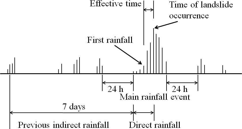
https://www.nat-hazards-earth-syst-sci.net/18/687/2018/nhess-18-687-2018-f01

Figure 1Definition of rainfall events based on effective accumulated rainfall (modified from Seo and Funasaki, 1973).

Download

2.3.2 Intensity of rolling rainfall (I_R)

Rainfall intensity refers to the amount of rainfall within a unit of time. It is considered a crucial index for evaluating disasters because greater intensity or longer durations have considerable impacts on slope stability. Furthermore, rainfall-induced landslides may be triggered by several hours of continuous rainfall. The raw rainfall data in this study were hourly precipitation; thus I_R (mm h⁻¹) can be expressed as follows:

\begin{matrix} (7) & I_{m R} = \sum_{t - m + 1}^{m} I = I_{t - m + 1} + I_{t - m + 2} + \dots + I_{t}, \end{matrix}

where I denotes rainfall intensity, m denotes the number of rolling hours of rainfall (set as 3 h in this study), I_mR denotes the I_R during m hours, and I_t denotes the rainfall intensity during hour t.

2.4 MHEM

The MHEM is a diverse non-linear mathematical model. Based on relative relationships, the MHEM presents an instability index (D_t) to indicate susceptibility in different areas. The objective is to estimate the variance of predisposing factors and then to determine the weight of each factor according to the value of variance, finally to derive a suitable landslide susceptibility assessment model (Su et al., 1998; Lin et al., 2009; Chue et al., 2015).

The predisposing factors in the MHEM are rated based on the frequency of landslide occurrence, which is calculated as follows:

\begin{matrix} (8) & R_{i} = \frac{r_{i}}{r_{T}}, \end{matrix}

where R_i represents the landslide pixel ratio of the various factors in class i, r_i represents the number of landslide pixels in class i, and r_T represents the total number of pixels. Thus, landslide percentage X_i is expressed as

\begin{matrix} (9) & X_{i} = \frac{R_{i}}{\sum R_{i}}, \end{matrix}

where X_i denotes the landslide percentage of class i and ΣR_i denotes the sum of the landslide pixel ratios.

Based on the landslide percentages of the various classes for each predisposing factor, the normalized score value of classes for each factor (d_n) can be calculated using Eq. (10), and presented in relative values ranging from 1 to 10.

\begin{matrix} (10) & d_{n} = \frac{9 (X_{i} - X_{min})}{(X_{max} - X_{min})} + 1 \end{matrix}

In Eq. (10), X_i represents the causal rate of the sample region, and X_max and X_min represent the maximum and minimum landslide percentages of the factor in the various sample regions.

To estimate the weight of influence of each predisposing factor, the coefficient of variation (V) of the landslide ratios derived from the class of the predisposing factors is used to represent the sensitivity of landslide ratios in different predisposing factor classes. A smaller coefficient of variation denotes higher similarity among the landslide probabilities in the various classes, which indicates that this factor grading method cannot determine which areas have higher or lower landslide probabilities. By contrast, a greater coefficient of variation denotes that this factor grading method can be used to describe the influence of factor classes on landslides. Thus, the coefficient of variation among the predisposing factors can indicate the factor weights. The coefficient of variation is calculated as shown in Eq. (11):

\begin{matrix} (11) & V = \frac{σ}{X} \times 100 %, \end{matrix}

where σ is the standard deviation and X is the mean landslide percentage of the various factor classes.

We divided the coefficient of variation of each individual factor by the total coefficient of variation of all factors to derive the factor weight, which represented the degree of influence of the factor on landslide occurrence. The factor weight can be calculated as shown in Eq. (12), where W is the factor weight and V is a coefficient of variation.

\begin{matrix} (12) & W_{i} = \frac{V_{i}}{V_{1} + V_{2} + \dots + V_{n}} \end{matrix}

Finally, the weight (W_i) of each factor is determined by the rank of its variance (V), and each factor is assigned a different weight. Subsequently, a non-linear mathematical model can be derived as follows:

\begin{matrix} (13) & D_{t} = d_{1}^{W_{1}} \times d_{2}^{W_{2}} \times d_{3}^{W_{3}} \times d_{4}^{W_{4}} \times d_{5}^{W_{5}} \dots \dots \times d_{n}^{W_{n}}, \end{matrix}

where D_t is the instability index of the samples, expressed using relative values ranging from 1 to 10. A cumulative value closer to 10 indicates greater landslide potential, whereas a cumulative value closer to 1 indicates lower landslide potential.

By using the concept of log-normal distribution in statistics, we converted the levels of instability index derived using the MHEM into probabilities of landslide occurrence. The calculation formula of the log-normal distribution is shown in Eq. (14):

\begin{matrix} (14) & P (F) = \frac{1}{x σ \sqrt{2 π}} e^{- \frac{1}{2} {[(\ln x - μ) / σ]}^{2}}, \end{matrix}

where x denotes the level of the instability index and μ and σ denote the mean and standard deviation of the level of the instability index. After calculating the probabilities of landslide occurrence by using the log-normal distribution, we normalized the probabilities to range from 0 to 1 for convenience. The normalization formula is shown in Eq. (15).

\begin{matrix} (15) & P {(F)}^{'} = \frac{(X_{i} - X_{min})}{(X_{max} - X_{min})} \end{matrix}

In Eq. (15), X_i represents the factor being normalized and X_max and X_min represent the maximum and minimum values of the factor, respectively.

3 Study area

We referred to the historical data on road disasters from the NCDR (National Science and Technology Center for Disaster Reduction, 2017) and considered road sections where rainfall-induced landslides occurred frequently in southern Taiwan. We focused on the periods before and after Typhoon Nanmadol (2011) and Typhoon Kong-rey (2013) hit southern Taiwan, and we selected part of the catchment area of Laonung River in southern Taiwan as our study area (Fig. 2), which includes areas from three districts in Kaohsiung city (Jiashian, Liouguei, and Taoyan). The Laonung River flows SW across the south of the study area and originates from the Jade Mountain. The study area is located in a tropical monsoon climate zone. According to the climate statistics (1983–2012) recorded by the Central Weather Bureau, the average annual rainfall is approximately 2758 mm. Provincial Highway 20 is in an east–west direction, the starting point of the highway is Tainan city in southern Taiwan, and the ending point is Degao Community in Guanshan town, Taitung County, with a total length of 203.982 km. Within the study area, Provincial Highway 20 starts from Liouguei District (76 K + 000) in the west and goes to Taoyan Village (87 K + 500) in the Taoyan District. According to the survey data from the Directorate General of Highways (2017), the road width of Provincial Highway 20 passing through the study area is about 8.8 m. The average traffic flow and the total number of vehicles carried per day for both directions are 2260 PCU (passenger car unit) and 1434. In the study area, most of the traffic vehicles are sedans, followed by trucks and buses.

https://www.nat-hazards-earth-syst-sci.net/18/687/2018/nhess-18-687-2018-f02

Figure 2Study area in the south of Taiwan. Purple line depicts the mountain road.

Download

4 Image interpretation and classification

4.1 Preprocessing of satellite images

This study employed and interpreted satellite images taken by FORMOSAT-2 (FM2). FM2 images have been extensively used to identify natural disasters and land use (e.g. Lin et al., 2004, 2006, 2011; Liu et al., 2007; Chen et al., 2009, 2013a). The FORMOSAT-2 satellite has a circular and sun synchronous orbit. With its high torque reaction wheels for all axes, the FORMOSAT-2 is able to point to a ±45^∘ along track and ±45^∘ across track and is thus able to capture any scene each day in all of Taiwan if necessary (Liu et al., 2007). FORMOSAT-2 images are available in 2 m resolution in panchromatic (pan) and 8 m in multispectral (ms) from visible to near-infrared with a coverage of 24 km×24 km. In the present study, prior to interpretation, the satellite images underwent spectral fusion, coordinate positioning, cropping, and cloud removal. The images taken by FM2 are multispectral with blue, green, red, and near-infrared (NIR) wavelengths (Chen et al., 2013a; Chue et al., 2015). Image fusion and coordinate positioning were conducted using the import data and coordinate positioning tool of ERDAS IMAGINE (2013). Then, we used the image analysis tool of ArcGIS to remove clouds from the images.

Table 2Error matrix of interpretation results of satellite images after Typhoon Kong-rey in 2013.

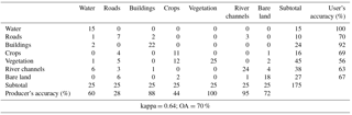
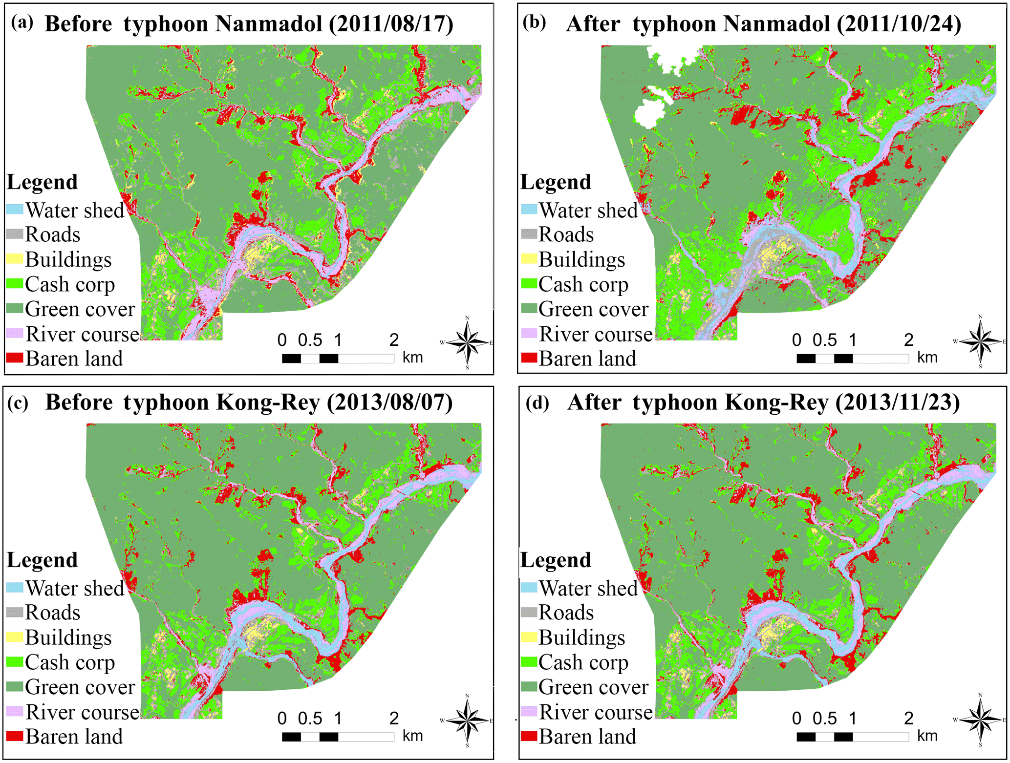
Download Print Version | Download XLSX

https://www.nat-hazards-earth-syst-sci.net/18/687/2018/nhess-18-687-2018-f03

Figure 3Interpretation and classification results of satellite images before (a, c) and after (b, d) Typhoon Nanmadol (a, b) and Typhoon Kong-rey (c, d).

Download

4.2 Training site selection and mapping

To map the sample areas required for image interpretation, we overlapped the high-resolution, preprocessed satellite images of the study area before and after the typhoons and mapped the training sites by using a GIS platform. Based on field investigations and relevant studies (Chen et al., 2009, 2013a; Chue et al., 2015), we selected areas with water, roads, buildings, crops, vegetation, river channels, and bare land within the study area as the sample area factors for interpretation training.

4.3 Image interpretation and accuracy assessment

Image interpretation and classification were conducted using the maximum likelihood module in ERDAS IMAGINE. The interpretation and classification results of the satellite images before and after Typhoon Nanmadol in 2011 and Typhoon Kong-rey in 2013 are shown in Fig. 3. The different colours in the images represent different interpretation factors.

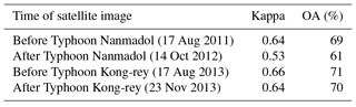
To verify the accuracy of the results, we randomly extracted 25 points from the satellite images for each training factor as checkpoints and tested the accuracy by using the aforementioned error matrix approach. With the satellite images before and after Typhoon Kong-rey in 2013 as an example, Table 2 shows the error matrix and accuracy assessment results of the satellite image interpretation and classification processes. Table 3 presents the kappa values and OA results of the satellite images captured before and after the two typhoons. As mentioned, kappa values ranging from 0.4 to 0.8 indicate moderate accuracy, and thus the interpretation results had moderate to high accuracy.

Taking the landslide inventory after Typhoon Kong-rey in 2013 as an example, there were 291 landslides, which totaled a landslide area around 135 ha. This was equivalent to an average concentration of 5.1 % throughout the whole study area of 2659 ha. Among the 291 landslides, 256 landslides were recognized with an area smaller than 1 ha, the remaining 35 landslides were recognized in the range of 1 to 8 ha. The biggest landslide, with an area around 7 ha.

5 Landslide susceptibility assessment

To evaluate the landslide susceptibility of slopes within the study area, we constructed 8 m×8 m grids by using the GIS platform along with the interpretation results of the two typhoons. We also constructed an 8 m×8 m digital elevation model (DEM) (SWCB, 2011) and input the classification results, thematic map of predisposing factors, and rainfall data into the pixel to aid subsequent landslide susceptibility assessments.

5.1 Predisposing factor selection and factor correlation test

5.1.1 Predisposing factor selection

Referring to Chen et al. (2009), we divided the predisposing factors of landslides into three categories: natural environment, land disturbance, and rainfall.

Natural environment factors

Elevation

The influence of elevation varies with the climate and thus affects the distribution of vegetation on the slope and type of weathering. In addition, elevation reflects the influence of geological structure, stress, and time. The highest and lowest elevations in the study area were 1481 and 365 m, respectively. Using the GIS platform, we extracted the elevation data from the DEM of the study area to estimate the mean elevation of each grid. We divided the elevation data into seven classes at intervals of 300 m.

Slope gradient

A slope's gradient generally exerts significant impact on slope stability. By using the DEM and gradient analysis of the GIS platform, we calculated the mean gradient of each pixel in the study area; subsequently, we divided the gradient values in the pixels within the study area into seven classes.

Aspect

Rainfall-induced landslides are subject to the influence of seasonal changes such as those related to rainfall and wind direction. Thus, the direction of the slope must be considered. As described, we used the DEM and aspect analysis function of the GIS platform to calculate the average aspect of the pixels in the study area. According to their direction, we divided them into six classes from windward to flat ground.

Table 3Interpretation results of satellite images before and after typhoons Nanmadol and Kong-rey.

Download Print Version | Download XLSX

Geology

Referring to the digital file of the Geologic Map of Taiwan, scale 1 : 50 000, Chiahsien, which was compiled by the Central Geological Survey of the Ministry of Economic Affairs in 2000, we determined that the geology of the study area includes five types of rock: the upper part of Changshan Formation, the Tangenshan Formation, the Changchihkeng Formation from the Miocene period, and modern alluvium and terrace deposits from the Holocene period. We divided geological strength into six classes (Chen et al., 2009).

Terrain roughness

Terrain roughness refers to the degree of change in pixel height. Wilson and Gallant (2000) proposed the use of the standard deviation of height within a radius to measure the degree of change in height because of its indicative meaning in relation to changes in regional height. Using the Neighborhood (focal statistics) of the Spatial Analyst Toolbox in ArcGIS, we calculated the terrain roughness of the DEM. Statistical cluster analysis was used to automatically divide terrain roughness into six classes.

Slope roughness

Slope roughness refers to the fluctuations in slope gradient in the pixels. High slope roughness means that the slope gradient varies considerably (Wilson and Gallant, 2000). Slope roughness is calculated through the same method as terrain roughness, except with the original elevation values being replaced with the slope gradient values obtained using ArcGIS. Just as terrain roughness was graded, we first used the Spatial Analyst Toolbox in ArcGIS to estimate the slope roughness of each pixel, after which we used cluster analysis to automatically divide slope roughness into six classes.

Distance to water

Streams will cause soil erosion and riparian erosion, which directly or indirectly affect the stability of the slope. We calculated the distances to water using the Buffer tool in ArcGIS and divided the distances into seven classes. Distance to road

The construction of the roads will also have an influence on the stability of the slope. Therefore, we also calculated the distances to road using the Buffer tool in ArcGIS and divided the distances into seven classes.

Land disturbance factors

Land disturbance varies with space and time. Based on the tendency to promote landslides, the index of land disturbance was developed, and we made some revisions to the qualitative approach proposed by Chen et al. (2009, 2013b) to calculate land disturbance and selected roads, buildings, crops, bare land, and vegetation as the land disturbance factors of landslides in the study area. We extracted the disaster and ground surface data from previous satellite image interpretation and classification results and input the land disturbance factors into the pixels by using the GIS platform. Referring to Chen et al. (2009, 2013b), the scores of the index for the disturbance condition (I_DC) in the pixels are assigned from five to one, corresponding to bare land, roads, buildings, crops, and vegetation.

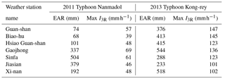
Table 4Effective accumulated rainfall and intensity of rolling rainfall observed at weather stations during Typhoon Nanmadol and Typhoon Kong-rey.

Download Print Version | Download XLSX

Rainfall factors

We collected precipitation data from weather stations of the Central Weather Bureau, including Guanshan, Biaohu, Hsiao Guanshan, Gaojhong, Sinfa, Jiashian, and Xinan. We then calculated the EAR and 3 h I_R (I_3R) levels observed at each station. The results from Typhoon Nanmadol in 2011 and Typhoon Kong-rey in 2013 are compiled in Table 4. By using the inverse distance weighting (IDW) function of ArcGIS and the EAR and maximum I_3R values of the weather stations, we estimated the rainfall of each pixel throughout the study area and then used cluster analysis to divide the results into six classes.

Table 5Correlation test results between the predisposing factors.

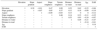
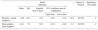
Download Print Version | Download XLSX

Table 6Paired sample t test results between elevation and terrain roughness and slope gradient and slope roughness.

Download Print Version | Download XLSX

5.1.2 Factor correlation test

To establish a landslide susceptibility assessment model, we selected elevation, slope gradient, aspect, geology, terrain roughness, slope roughness, distance to water, distance to road, I_DC, and rainfall as landslide-predisposing factors. Rainfall included EAR and maximum I_3R.

We employed the Pearson correlation test tool in SPSS software (2005) to examine the correlation among these factors. The correlation coefficients ranged from −1 to +1, with +1, −1, and 0 indicating complete positive correlation, complete negative correlation, and no correlation between two variables, respectively. Factors with high correlation were then subjected to a paired sample t test conducted using SPSS to examine the significance of the correlation between them. Those with high correlation were eliminated.

Table 5 presents the test results regarding the correlation between the predisposing factors. As shown, the degree of correlation between most factors was moderate to low. A high degree of correlation was found only between elevation and terrain roughness and between slope gradient and slope roughness. Thus, we administered paired sample t tests to these two factor pairs to test the significance of the correlation. The results in Table 6 show that the significance was 0 (<0.05) for the correlation between both pairs, indicating no correlation; thus these factors were not eliminated.

5.2 Landslide susceptibility assessment and hazard map

To apply the MHEM in order to establish a landslide susceptibility assessment model, we input the natural environment, land disturbance, and rainfall factors into the pixels by using the GIS platform. By using the changes in bare land between the images before and after the typhoons and applying image subtraction aided by manual checking, we obtained the pixel data of the rainfall-induced landslide locations in the study area. With the study area after Typhoon Nanmadol in 2011 as an example, we examined EAR during the rainfall period and rated the classes by using the factor weights derived using the MHEM, as shown in Table A1 of Appendix A.

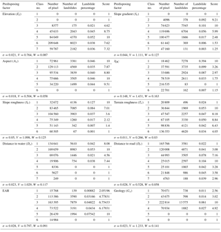
The calculation process is explained in this paper using elevation as an example. In accordance with factor selection, the elevation factor was divided into seven classes. Aided by the GIS platform, we calculated the total number of pixels, total number of landslides, and landslide percentage within each elevation level in the study area by using Eqs. (8) and (9). Based on the landslide percentages of the elevation factor and the minimum and maximum landslide percentages, we subsequently obtained the scores of the factors by using Eq. (10). We then calculated the standard deviation, coefficient of variation, and weight values by using Eqs. (11) and (12); the results are listed in Table A1 of Appendix A. The presented results show that the standard deviation (σ), coefficient of variation (V), and factor weight (W) of the landslide percentage were 0.021, 0.764, and 0.087, respectively. Finally, we calculated the instability indices by using the weight values and scores of the factors through Eq. (13). Furthermore, the results in Table A1 of Appendix A indicate that the degrees of land disturbance (I_DC), geology (G_s), slope gradient (S_s), and slope roughness had the greatest influence on landslides in the study area, followed by distance to water (D_s), EAR, and elevation (E_l).

Table 7Intervals of instability index and landslide probability of rainfall factors.

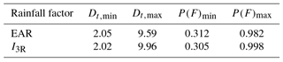
Download Print Version | Download XLSX

For EAR and I_3R we used an instability index to determine the level of landslide susceptibility of slopes throughout the study area. The derived instability index intervals (Table 7) for EAR and I_3R ranged from 2.05 to 9.59 and 2.02 to 9.96. By using Eqs. (14) and (15), the landslide probability intervals calculated based on EAR and I_3R are presented in Table 7.

We employed the mean probability of landslide occurrence to differentiate between high and low landslide susceptibility. Landslides were considered more likely to occur in areas where the probability of landslide occurrence was greater than the mean. By contrast, landslides were considered less likely to occur in areas where the probability of landslide occurrence was lower than the mean. With rainfall factor EAR as an example, we determined the mean probability of landslide occurrence to be 0.46. We further divided landslide susceptibility into four levels: high (0.731–1), medium high (0.461–0.73), medium low (0.23–0.46), and low (0–0.23). The results showed that the mean probability of landslide occurrence varied little, regardless of whether it was calculated using EAR or I_3R.

Table 8Accuracy of landslide susceptibility map for different rainfall factors and typhoons.

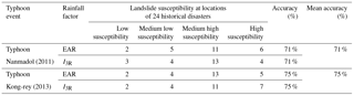
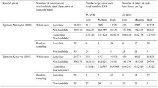
Download Print Version | Download XLSX

Table 9Numbers of landslide pixels in the study correspond to different D_t levels under different rainfall factors after typhoons.

Download Print Version | Download XLSX

By using the GIS platform, we considered the landslide susceptibility calculated using EAR for Typhoon Nanmadol in 2011 as an example. As illustrated in Fig. 4, we included an overlay created by the NCDR showing the locations of historical disasters within the study area. The results revealed a total of 24 historical disasters, 17 of which were situated in areas of medium high or high landslide susceptibility. Therefore, the estimation accuracy in this study was approximately 71 %. Regarding Typhoon Kong-rey in 2013, 18 historical disasters occurred within areas of medium high or high landslide susceptibility, thereby yielding 75 % accuracy. Table 8 presents the accuracy levels associated with using different rainfall factors to calculate landslide susceptibility for different typhoons.

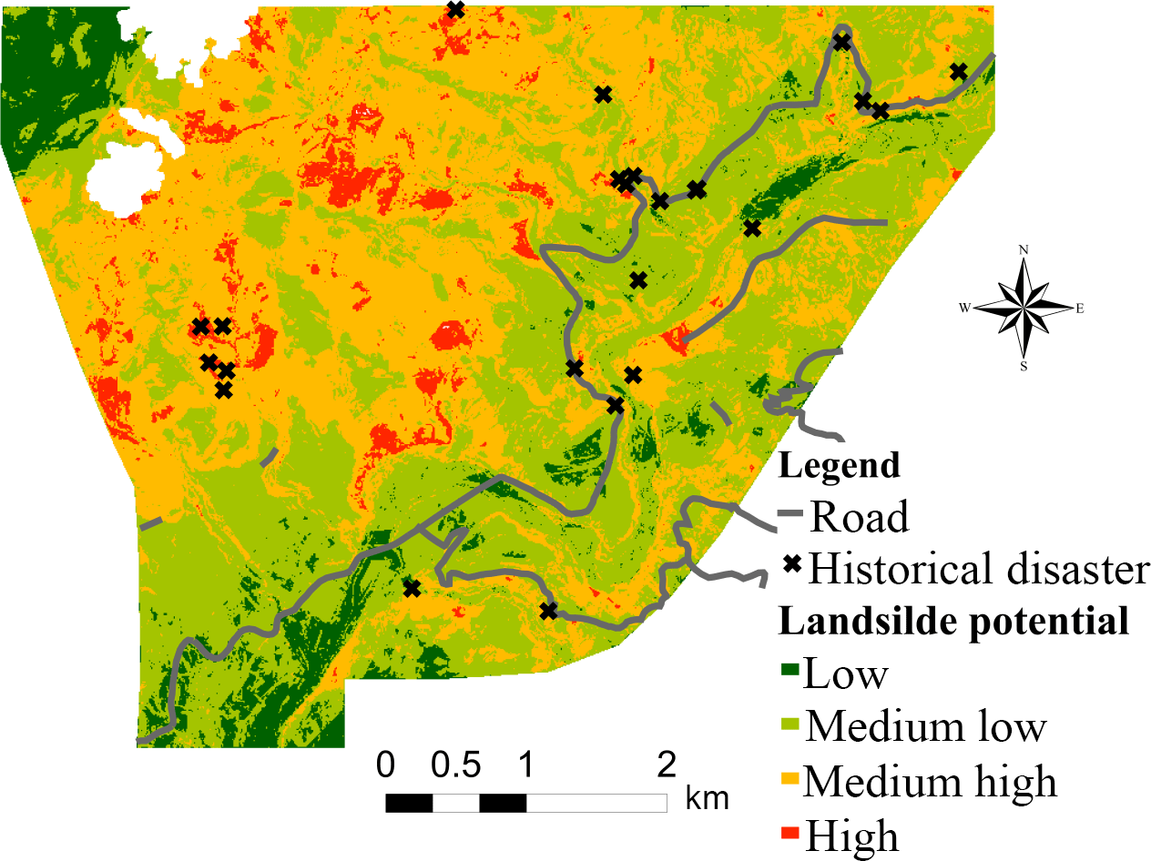
https://www.nat-hazards-earth-syst-sci.net/18/687/2018/nhess-18-687-2018-f04

Figure 4Landslide susceptibility in the study area, in which cross symbols represent the historical disasters collected from NCDR (2017).

Download

https://www.nat-hazards-earth-syst-sci.net/18/687/2018/nhess-18-687-2018-f05

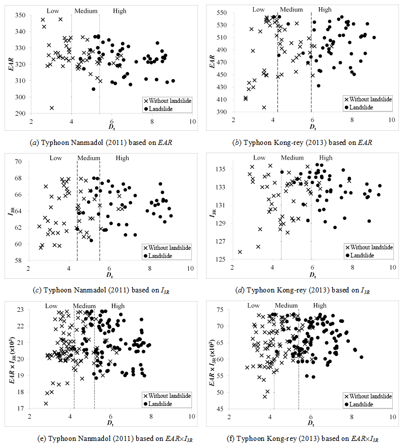
Figure 5Relationships among instability index, effective accumulated rainfall, and landslide occurrence in the study area after typhoons Nanmadol (2011) and Kong-rey (2013).

Download

5.3 Investigation of rainfall factors and instability index

To understand the relationship between the rainfall factors and the degree of instability on the slopes in the study area after the typhoons, we first removed the cloud cover grids from post typhoon images and subsequently employed cluster analysis to divide the instability indices of the pixels into three levels: high, medium, and low. We then collected random samples based on the proportions of landslide and non-slide pixels at each level (50 landslide and 50 non-landslide pixel points) and plotted their relationship. Table 9 and Fig. 5a–d present the relationships between the rainfall factors (EAR and I_3R), instability index, and landslide occurrence in the pixels following Typhoon Nanmadol in 2011 and Typhoon Kong-rey in 2013. Figure 5a and b show EAR, whereas Fig. 5c and d show I_3R. The presented results indicate that the typhoon events increased the degree of slope instability (D_t) and landslide occurrence, regardless of whether EAR or I_3R was considered. Furthermore, significantly more landslide points were situated in areas of high instability than in areas of other levels of instability, and landslides rarely occurred in areas of low instability. Moreover, areas of high slope instability were prone to landslides even if their EAR or I_3R was low. By contrast, areas of low instability required more rainfall for the occurrence of landslides. The results (Table 9) further showed that the EAR and I_3R levels of Typhoon Kong-rey in 2013 were greater than those of Typhoon Nanmadol in 2011. Thus, at any D_t level, the proportion of landslides that occurred in the study area after Typhoon Kong-rey was higher than that after Typhoon Nanmadol. Figure 5e and f present the relationships between EAR×I_3R, the instability index, and landslide occurrence; EAR×I_3R is the index of rainfall-induced landslide (ILR), with a higher value indicating higher susceptibility to a landslide. The figures show that for a high instability index, even a small rainfall event could trigger a landslide (lower-right corners of the figures). By contrast, for a low instability index, a larger rainfall event could not easily trigger a landslide (upper-left corners of the figures).

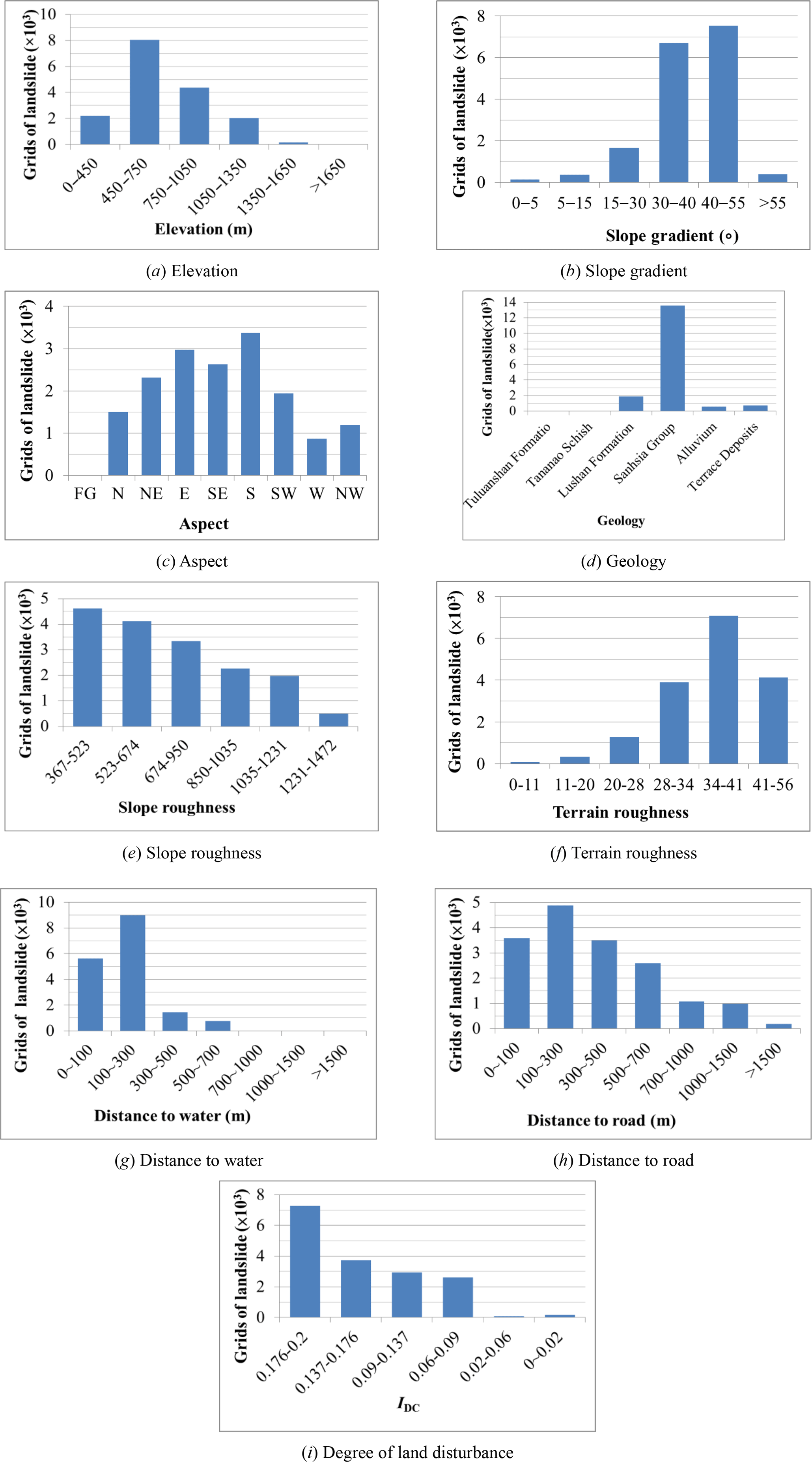
https://www.nat-hazards-earth-syst-sci.net/18/687/2018/nhess-18-687-2018-f06

Figure 6Relationships between landslide predisposing factors and number of landslide pixels in the study area.

Download

https://www.nat-hazards-earth-syst-sci.net/18/687/2018/nhess-18-687-2018-f07

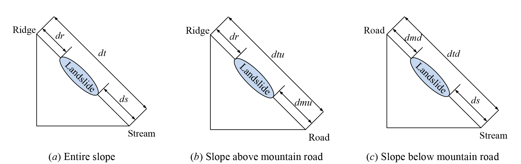
Figure 7Diagrams of landslide area on slope, in which d_r represents the distance between the highest point of a landslide area and the nearest ridge, d_s the distance between the lowest point of the landslide area and the nearest stream, and d_t the distance between ridge and stream.

Download

6 Landslide location analysis

We analysed the spatial characteristics of landslides by using landslide locations collected from before and after the two typhoons and the land surface interpretation results of the study area.

6.1 Investigation of landslide predisposing factors and landslide area

The influence of predisposing factors on landslides varies. In this study, we examined the relationships between landslide area and various predisposing factors. By using the area of landslides (i.e. the number of landslide pixels) induced by Typhoon Nanmadol in 2011 as an example, we investigated the influences of the predisposing factors (elevation, slope gradient, aspect, geology, slope roughness, terrain roughness, distance to water, distance to road, and degree of land disturbance) on landslides. The various factor classes and corresponding numbers of landslide pixels are shown in Fig. 6a–i.

Figure 6a presents the relationship between different classes of elevation and the number of landslide pixels (landslide area). As shown in the figure, the number of landslide pixels in the study area peaked at elevations between 450 and 750 m and then declined as the elevation increased. Figure 6b displays the relationship between different classes of slope gradient and the number of landslide pixels (landslide area). As shown in the figure, the number of landslide pixels in the study area increased with the slope gradient and peaked between 30 and 55^∘. Landslides rarely occurred on slopes steeper than 55^∘. Figure 6c illustrates the relationship between aspect and the number of landslide pixels, with aspect divided into eight categories: north, north-east, east, south-east, south, south-west, west, and north-west. As shown in the figure, the number of landslide pixels was highest on slopes facing south, followed by those on slopes facing east and south-east. We speculate that this is because rainfall during the typhoon season in Taiwan promotes poor cementation and high weathering on slopes along rivers, which consequently prompts these slopes to develop toward low-lying rivers (which run from the north-east to the south-west) after rainfall events.

Figure 6d shows the relationship between geology and the number of landslide pixels. As shown in the figure, the Sanhsia Group and its stratigraphic equivalence lead to landslides more easily than the Lushan Formation in the study area. The Sanhsia Group and its stratigraphic equivalence mainly comprise sandstone, shale, and interbedded sandstone and shale. Shale has weaker cementation, lower strength, and a greater tendency to weather and fracture. By contrast, the Lushan Formation consists of argillite, slate, and interbedded argillite and sandstone, and its strength is controlled by cleaving; some areas are prone to weathering and fracturing. Thus, both rock types are more likely to collapse, but on the whole, the Sanhsia Group and its stratigraphic equivalence collapse more easily than the Lushan Formation. Furthermore, this result indicates that the locations of landslide areas within the study area are associated with geology. Figure 6e presents the relationship between slope roughness and the number of landslide pixels. The number of landslide pixels within a level of slope roughness first increased with the slope roughness and then began to decline once a certain level of slope roughness (35–40) was reached. This result is similar to that of the influence of the slope gradient on the number of landslide pixels. Figure 6f displays the relationship between terrain roughness and the number of landslide pixels. As shown in this figure, the results are similar to those regarding the influence of elevation on the number of landslide pixels: the number of pixels declined when the terrain roughness was greater than 500 and was very small when the terrain roughness was greater than 1200.

Figure 6g illustrates the relationship between distance to water and the number of landslide pixels. The presented results show a significantly greater number of landslide pixels within 300 m of water. The width of the river channel within the study area was determined to range from 100 to 200 m, revealing that the development of landslide areas near water in the study area is caused by rainfall significantly raising the water level in the river, which scours the slope toe, affects slope stability, and triggers landslides. Figure 6h presents the relationship between distance to road and the number of landslide pixels. The presented results reveal that areas between 100 and 300 m from roads had the greatest number of landslide pixels. Further examination of the relationship between distance to road and the area and number of landslides revealed that most landslides between 0 and 100 m from roads were small collapses, whereas those between 100 and 300 m from roads were larger in area. The number of landslides 0–100 m from roads was greater than that 100–300 m from roads.

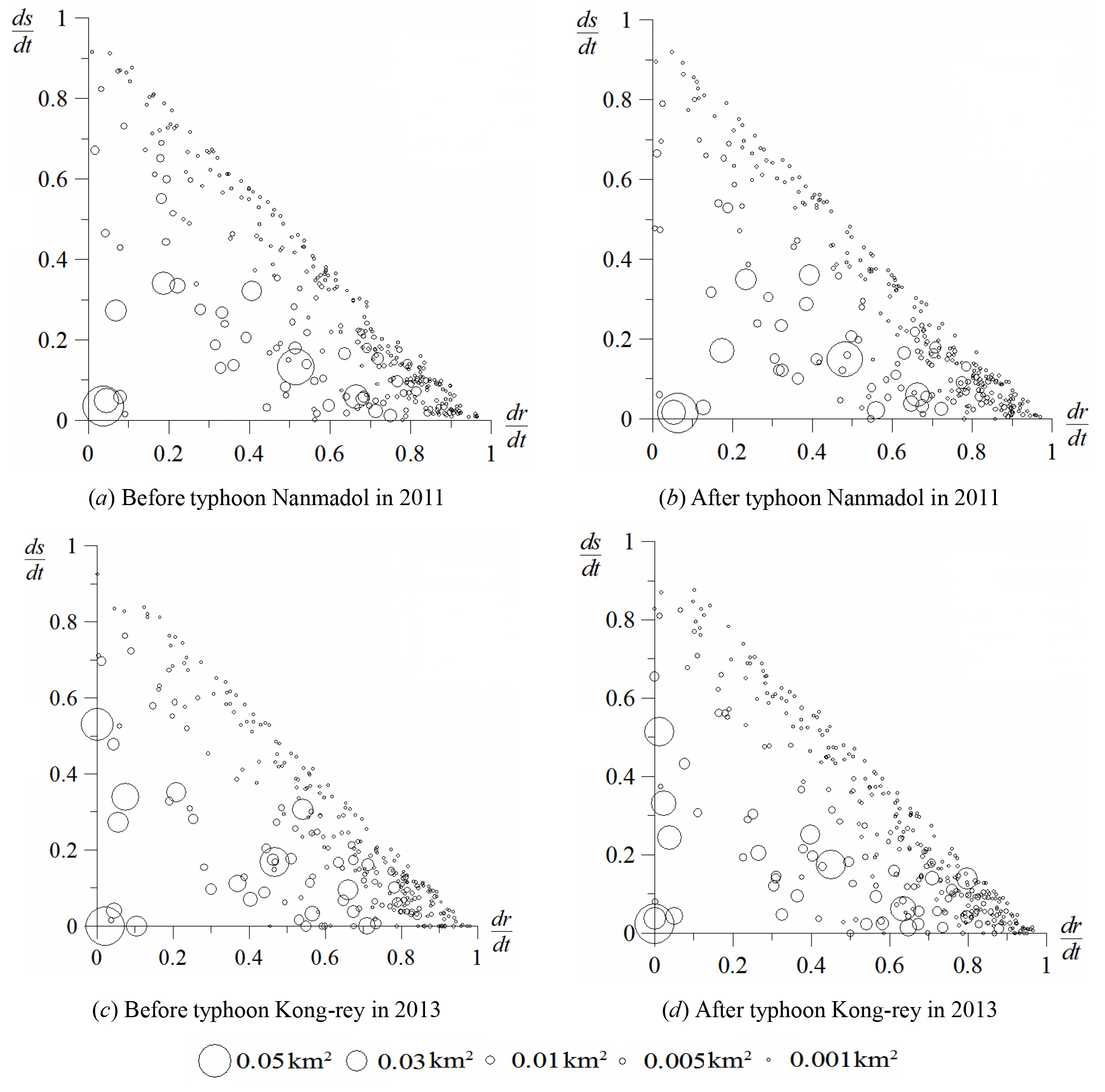
https://www.nat-hazards-earth-syst-sci.net/18/687/2018/nhess-18-687-2018-f08

Figure 8Spatial distribution of bare land in the study area before and after the typhoons Nanmadol (top) and Kong-rey (bottom). The sizes of the bubbles reflect the areas of bare land.

Download

The degree of land disturbance can represent the changes in surface conditions including roads, buildings, crops, bare land, and vegetation. A greater degree of land disturbance likely indicates a greater degree of surface changes, which can yield a greater number of landslide pixels. Figure 6i shows the relationship between the degree of land disturbance and the number of landslide pixels. The presented results indicate that the number of landslide pixels increased with the degree of land disturbance.

6.2 Landslide scale and spatial distribution

We employed the terrain tool in ERDAS IMAGINE and the DEM to identify the ridges and valleys in the study area. Following the methods in previous studies (Meunier et al., 2008; Chue et al., 2015), we extracted the distances between the highest point of a landslide area and the nearest ridge (d_r), between the lowest point of the landslide area and the nearest stream (d_s), and between the ridge and the stream (d_t) (Fig. 7). Furthermore, in Taiwan, many slopes are visible on developed mountain roads built between ridges and streams. Therefore, we explored the spatial distribution of landslides above and below mountain roads. Similarly to Fig. 7a, to explore the spatial distribution of landslides, we extracted the distances between the highest point of a landslide area on a slope above a road and the nearest ridge (d_r), between the lowest point of the landslide area and the nearest mountain road (d_mu), and between the ridge and the mountain road (d_tu) (Fig. 7b). We also investigated this distribution by extracting the distances between the highest point of a landslide area on a slope below a road and the nearest mountain road (d_md) between the lowest point of the landslide area and the nearest stream (d_s) and between the mountain road and the stream (d_td) (Fig. 7c).

This study examined the spatial distribution of landslides in the region along Provincial Highway 20 before and after Typhoon Nanmadol in 2011 and Typhoon Kong-rey in 2013. Using the approach shown in Fig. 7a, we mapped the bare land in the study area, as shown in Fig. 8a–d. Of these figures, Fig. 8a and c show the conditions before the typhoons, whereas Fig. 8b and d present the conditions after the typhoons. The presence of bare locations near the Y axis ( $d_{r} / d_{t} \approx 0$ ) denotes that the bare land originated near the ridge. By contrast, the presence of bare locations near the X axis ( $d_{s} / d_{t} \approx 0$ ) denotes that the bare land progressed toward the stream. Thus, the presence of bare locations near the origin denotes that the bare land originated near the ridge and progressed toward the stream.

The results in Fig. 8a–d show more bare locations in the lower-right halves of the graphs, some of which are larger in area. The figures indicate fewer bare locations in the upper-left halves of the graphs, and the ones that are present are smaller in area. These spatial distribution characteristics are similar to those derived by Meunier et al. (2008). We speculate that this is because the frequency of rainfall-induced landslides increases significantly because of bank erosion, which is shown in the lower-right half of Fig. 8 ( $d_{r} / d_{t} \geq 0.5$ and $d_{s} / d_{t} \leq 0.5$ ). Furthermore, the bare locations before and after typhoons Nanmadol and Kong-rey show that the bare land does not increase in number but increases significantly in area, implying that old landslides may result in more collapses or expansions of the affected area. In addition, the number of old landslides is greater than that of new landslides.

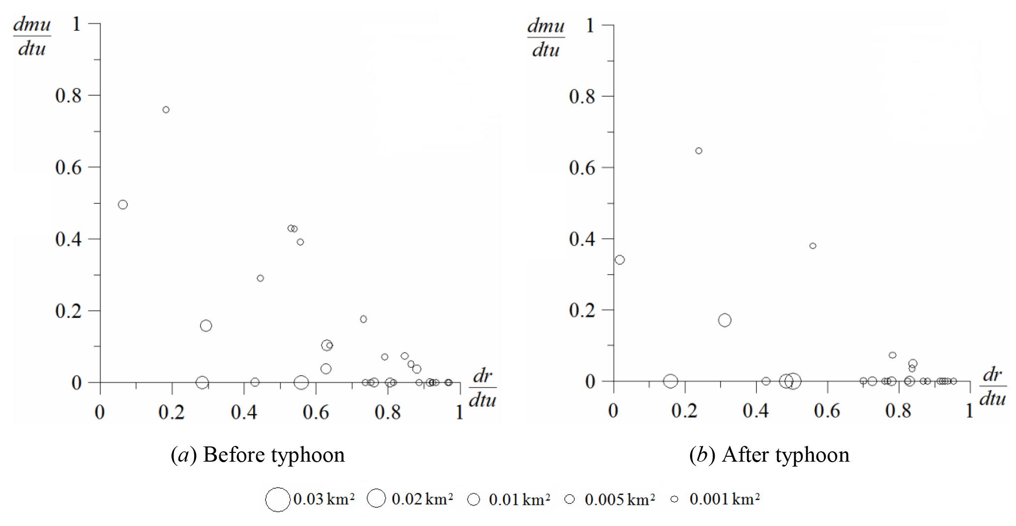
https://www.nat-hazards-earth-syst-sci.net/18/687/2018/nhess-18-687-2018-f09

Figure 9Spatial distribution of bare land on slopes above mountain roads in the study area before and after Typhoon Kong-rey in 2013. The sizes of the bubbles reflect the areas of bare land.

Download

We explored the spatial distribution of landslides on slopes above (Fig. 9) and below (Fig. 10) mountain roads in the study area before and after Typhoon Kong-rey in 2013. Figures 9a and 10a present the spatial distribution of bare land before the typhoon, whereas Figs. 9b and 10b present the spatial distribution of bare land after the typhoon.

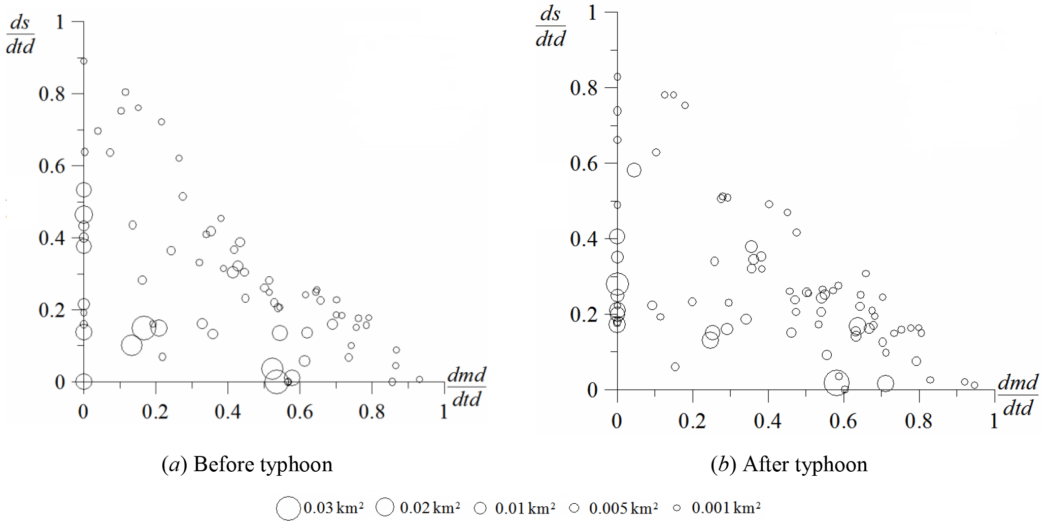
https://www.nat-hazards-earth-syst-sci.net/18/687/2018/nhess-18-687-2018-f10

Figure 10Spatial distribution of bare land on slopes below mountain roads in the study area before and after Typhoon Kong-rey in 2013. The sizes of the bubbles reflect the areas of bare land.

Download

As shown in Fig. 9, most landslides on the slopes above the mountain roads occurred close to the roads, most likely because road construction involves cutting the slope toe and increasing the gradient. After the typhoon, the bare locations on the slopes above the roads in the study area did not increase in number significantly; thus rainfall did not exert a substantial impact on the slopes above the roads. The results in Fig. 10 show bare locations on the slopes below the mountain roads developing from near the roads to the streams. The bare locations near the streams may also have been affected by rainfall-induced bank erosion. However, the bare land near the roads may have been a result of roads being constructed in the study area, which affects slope stability and increases the probability of landslides. Furthermore, the bare locations near the roads slightly increased in number after the typhoon, likely because the roads changed the routes of surface run-off. The area of bare land near the streams also increased, possibly because the water flow scours the slope toe and causes continual bank collapses. Thus, typhoons have a significant impact on the stability of slopes below mountain roads.

7 Conclusions

This study applied the maximum likelihood method to interpret and classify satellite images before and after two typhoons in 2011 and 2013. We extracted landslide and land use information from the areas surrounding roads and then compiled the rainfall and DEM data from the typhoon events. By using the MHEM, we established a landslide susceptibility assessment model and examined the relationships between predisposing factors and the area and number of landslides within the study area, as well as the relationships between roads and the spatial distribution of landslides. The results show that the kappa coefficients associated with the use of the maximum likelihood method to interpret and classify satellite images before and after Typhoon Nanmadol in 2011 and Typhoon Kong-rey in 2013 ranged from 0.53 to 0.66, whereas the OA ranged from 61 to 71 %, indicating moderately high accuracy. According to the results of the instability index-based landslide susceptibility assessment model, the degree of land disturbance, geology, slope gradient, and slope roughness had the greatest impacts on landslides. A comparison of historical landslides triggered by the typhoons and the results of the hazard map revealed 71 % accuracy for Typhoon Nanmadol in 2011 and 75 % accuracy for Typhoon Kong-rey in 2013. Regarding the influence of the predisposing factors, an elevation of 450–750 m, a slope gradient of 30–55^∘, and distances within 300 m of water or roads were associated with a larger scale of landslides. The scale of landslides also increased with the degree of land disturbance. The relationships between the ILR, instability index, and landslide occurrence indicate that for a high instability index, even a smaller rainfall event could trigger a landslide. By contrast, for a low instability index, a larger rainfall event could not easily trigger a landslide. Thus, the instability index can effectively reflect landslide susceptibility. Comparisons of the distribution of bare land before and after typhoon events showed that most landslides in the study area were caused by stream water scouring away the toes of bank slopes. Although bare locations did not significantly increase in number after the typhoon events, they increased significantly in area, implying that the number of old landslide areas holding more collapses or expansions was greater than that of new landslide areas developing. In addition, the results obtained from observing changes on slopes above and below mountain roads after the typhoon events indicate that the number of bare locations on the slopes above the roads in the study area did not increase significantly, whereas the bare locations near the roads on the slopes below the roads slightly increased in number after the typhoon events, likely because of the roads changing the routes of surface run-off. The amount of bare land near streams also increased, possibly because the water flow scours the slope toe.

Data availability

The data sets of geology data, rainfall data, satellite images, and topography data can be provided on request from the institutions and projects mentioned in the acknowledgements.

Appendix A

Table A1Weights and scores of predisposing factors after rainfall brought by Typhoon Nanmadol in 2011.

Download Print Version | Download XLSX

Competing interests

The authors declare that they have no conflict of interest.

Special issue statement

This article is part of the special issue “Landslide–road network interactions”. It is not associated with a conference.

Acknowledgements

This work is funded by the Soil and Water Conservation Bureau, Taiwan, Republic of China and by the grant MOST 105-2625-M-309-002, MOST 105-2625-M-309-003 from the Ministry of Science and Technology, Taiwan, Republic of China

Edited by: Faith Taylor
Reviewed by: two anonymous referees

References

Akgün, A., Dag, S., and Bulut, F.: Landslide susceptibility mapping for a landslide prone area (Findikli, NE of Turkey) by likelihood-frequency ratio and weighted linear combination models, Environ. Geol., 54, 1127–1143, https://doi.org/10.1007/s00254-007-0882-8, 2008.

Ali, A., Huang, J., Lyamin, A. V., Sloan, S. W., and Cassidy, M. J.: Boundary effects of rainfall-induced landslides, Comput. Geotech., 61, 351–354, https://doi.org/10.1016/j.compgeo.2014.05.019, 2014.

Anbalagan, D.: Landslide hazard evaluation and zonation mapping in mountainous terrain, Eng. Geol., 32, 269–277, https://doi.org/10.1016/0013-7952(92)90053-2, 1992.

Ayalew, L. and Yamagishi, H.: The application of GIS-based logistic regression for landslide susceptibility mapping in the Kakuda–Yahiko Mountains, Central Japan, Geomorphology, 65, 15–31, https://doi.org/10.1016/j.geomorph.2004.06.010, 2005.

Ayalew, L., Yamagishi, H., Marui, H., and Kanno, T.: Landslides in Sado Island of Japan: Part II. GIS-based susceptibility mapping with comparisons of results from two methods and verifications, Eng. Geol., 81, 432–445, https://doi.org/10.1016/j.enggeo.2005.08.004, 2005.

Baeza, C. and Corominas, J.: Assessment of shallow landslide susceptibility by means of multivariate statistical techniques, Earth Surf. Proc. Land., 26, 1251–1263, https://doi.org/10.1002/esp.263, 2001.

Bai, S. B., Wang, J., Lu, G. N., Zhou, P. G., Hou, S. S., and Xu, S. N.: GIS-based and data-driven bivariate landslide susceptibility mapping in the Three George area, China, Pedosphere, 19, 14–20, https://doi.org/10.1016/S1002-0160(08)60079-X, 2009.

Barredo, J. I., Benavides, A., Hervas, J., and vanWesten, C. J.: Comparing heuristic landslide hazard assessment techniques using GIS in the Tirajana basin, Gran Canaria Island, Spain, Int. J. Appl. Earth Obs. Geoinf., 2, 9–23, https://doi.org/10.1016/S0303-2434(00)85022-9, 2000.

Brabb, E. E.: Innovative approaches to landslide hazard and risk mapping, Proceedings of the Fourth International Symposium on Landslides, Canadian Geotechnical Society, Toronto, Canada, 1, 307–324, 1984.

Bruzzone, L. and Prieto, D. F.: Unsupervised retraining of a maximum likelihood classifier for the analysis of multitemporal remote sensing images, IEEE T. Geosci. Remote, 39, 456–460, https://doi.org/10.1109/36.905255, 2001.

Carrara, A., Crosta, G., and Frattini, P.: Geomorphological and historical data in assessing landslide hazard. Earth Surf. Proc. Land., 28, 1125–1142, https://doi.org/10.1002/esp.545, 2003.

Carrara, A., Crosta, G., and Frattini, P.: Comparing models of debris-flow susceptibility in the alpine environment, Geomorphology, 94, 353–378, https://doi.org/10.1016/j.geomorph.2006.10.033, 2008.

Central Weather Bureau (CWB): Ministry of Transportation and Communications (MOTC), Executive Yuan, R. O. C. (Taiwan), available at: http://www.cwb.gov.tw/V7/knowledge/encyclopedia/ty038.htm (last access: 1 August 2017), 2017 (in Chinese).

Chadwick, J., Dorsch, S., Glenn, N., Thackray, G., and Shilling, K.: Application of multi-temporal high-resolution imagery and GPS in a study of the motion of a canyon rim landslide, ISPRS, J. Photogramm. Eng. Rem. S., 59, 212–221, https://doi.org/10.1016/j.isprsjprs.2005.02.001, 2005.

Chang, K. T., Chiang, S. H., and Lei, F.: Analysing the relationship between typhoon-triggered landslides and critical rainfall conditions, Earth Surf. Proc. Land., 33, 1261–1271, https://doi.org/10.1002/esp.1611, 2007.

Chen, L., Wei, H. P., and Chen, H. M.: A study of applying supervised classifications for remote sensing imagery recognition techniques, J. Taiwan Agric. Eng., 50, 59–70, 2004 (in Chinese).

Chen, C. Y., Chen, T. C., Yu, F. C., Yu, W. H., and Tseng, C. C.: Rainfall duration and debris-flow initiated studies for real-time monitoring, Environ. Geol., 47, 715–724, https://doi.org/10.1007/s00254-004-1203-0, 2005.

Chen, Y. R., Chen, J. W., Hsieh, S. C., and Ni, P. N.: The application of remote sensing technology to the interpretation of land use for rainfall-induced landslides based on genetic algorithms and artificial neural networks, IEEE J. Sel. Top. Appl., 2, 87–95, https://doi.org/10.1109/JSTARS.2009.2023802, 2009.

Chen, J. W., Chue, Y. S., and Chen, Y. R.: The application of genetic adaptive neural network in landslide disaster assessment, J. Mar. Sci. Technol., 21, 442–452, https://doi.org/10.6119/JMST-012-0709-2, 2013a.

Chen, Y. R., Ni, P. N., and Tsai, K. J.: Construction of a sediment disaster risk assessment model, Environ. Earth Sci., 70, 115–129, https://doi.org/10.1007/s12665-012-2108-y, 2013b.

Chue, Y. S., Chen, J. W., and Chen, Y. R.: Rainfall-induced slope landslide potential and landslide distribution characteristics assessment, J. Mar. Sci. Technol., 23, 705–716, https://doi.org/10.6119/JMST-015-0529-3, 2015.

Cohen, J.: A coefficient of agreement for nominal scales, Educ. Psychol. Meas., 20, 37–46, https://doi.org/10.1177/001316446002000104, 1960.

Congalton, R. G.: A review of assessing the accuracy of classifications of remotely sensed data, Remote Sens. Environ., 37, 35–46, https://doi.org/10.1016/0034-4257(91)90048-B, 1991.

Constantin, M., Bednarik, M., Jurchescu, M. C., and Vlaicu, M.: Landslide susceptibility assessment using the bivariate statistical analysis and the index of entropy in the Sibiciu Basin (Romania), Environ. Earth Sci., 63, 397–406, https://doi.org/10.1007/s12665-010-0724-y, 2011.

Crozier, M. J. and Eyles, R. J.: Assessing the probability of rapid mass movement, in: The New Zealand Institution of Engineers – Proceedings of Technical Groups, Proc. Third Australia–New Zealand Conference on Geomechanics, Wellington, 2.47–2.51, 1980.

Dadson, S. J., Hovius, N., Chen, H., Dade, W. B., Lin, J. C., Hsu, M. L., Lin, C. W., Horng, M. J., Chen, T. C., Milliman, J., and Stark, C. P.: Earthquake triggered increase in sediment delivery from an active mountain belt, Geology, 32, 733–736, https://doi.org/10.1130/G20639.1, 2004.

Dai, F. C. and Lee, C. F.: Frequency-volume relation and prediction of rainfall-induced landslides, Eng. Geol., 59, 253–266, https://doi.org/10.1016/S0013-7952(00)00077-6, 2002.

Das, I., Sahoo, S., Westen, C., Stein, A., and Hack, R.: Landslide susceptibility assessment using logistic regression and its comparison with a rock mass classification system, along a road section in the northern Himalayas (India), Geomorphology, 114, 627–637, https://doi.org/10.1016/j.geomorph.2009.09.023, 2010.

Das, I., Stein, A., Kerle, N., and Dadhwal, V. K.: Landslide susceptibility mapping along road corridors in the Indian Himalayas using Bayesian logistic regression models, Geomorphology, 179, 116–125, https://doi.org/10.1016/j.geomorph.2012.08.004, 2012.

Devkota, K. C., Regmi, A. D., Pourghasemi, H. R., Yoshida, K., Pradhan, B., Ryu, I. C., Dhital, M. R., and Althuwaynee, O. F.: Landslide susceptibility mapping using certainty factor, index of entropy and logistic regression models in GIS and their comparison at Mugling–Narayanghat road section in Nepal Himalaya, Nat. Hazards, 65, 135–165, https://doi.org/10.1007/s11069-012-0347-6, 2013.

Directorate General of Highways (DGH): Ministry of Transportation and Communications (MOTC), Executive Yuan, R. O. C. (Taiwan), available at: https://www.thb.gov.tw/sites/ch/modules/download/download_list?node=bcc520be-3e03-4e28-b4cb-7e338ed6d9bd&c=83baff80-2d7f-4a66-9285-d989f48effb4 (last access: 15 June 2017), 2017 (in Chinese).

Erbek, S. F., Ozkan, C., and Taberner, M.: Comparison of maximum likelihood classification method with supervised artificial neural network algorithms for land use activities, Int. J. Remote Sens., 25, 1733–1748, https://doi.org/10.1080/0143116031000150077, 2004.

Giannecchini, R.: Relationship between rainfall and shallow landslides in the southern Apuan Alps (Italy), Nat. Hazards Earth Syst. Sci., 6, 357–364, https://doi.org/10.5194/nhess-6-357-2006, 2006.

Giannecchini, R., Galanti, Y., and D'Amato Avanzi, G.: Critical rainfall thresholds for triggering shallow landslides in the Serchio River Valley (Tuscany, Italy), Nat. Hazards Earth Syst. Sci., 12, 829–842, https://doi.org/10.5194/nhess-12-829-2012, 2012.

Gökceoglu, C. and Aksoy, H.: Landslide susceptibility mapping of the slopes in the residual soils of the Mengen region (Turkey) by deterministic stability analyses and image processing techniques, Eng. Geol., 44, 147–161, https://doi.org/10.1016/S0013-7952(97)81260-4, 1996.

Greco, R., Sorriso-Valvo, M., and Catalano, E.: Logistic regression analysis in the evaluation of mass movements susceptibility: the Aspromonte case study, Calabria, Italy, Eng. Geol., 89, 47–66, https://doi.org/10.1016/j.enggeo.2006.09.006, 2007.

Guimarães, R. F., Montgomery, D. R., Greenberg, H. M., Fernandes, N. F., Gomes, R., and Abilio de Carvalho Júnior, O.: Parameterization of soil properties for a model of topographic controls on shallow landsliding: application to Rio de Janeiro, Eng. Geol., 69, 99–108, https://doi.org/10.1016/S0013-7952(02)00263-6, 2003.

Gupta, R. P. and Anbalagan, R.: Slope stability of Theri dam reservoir area, India, using landslide hazard zonation (LHZ) mapping, Q. J. Eng. Geol., 30, 27–36, https://doi.org/10.1144/GSL.QJEGH.1997.030.P1.03, 1997.

Guzzetti, F., Carrara, A., Cardinali, M., and Reichenbach, P.: Landslide hazard evaluation: a review of current techniques and their application in a multi-scale study, Central Italy, Geomorphology, 31, 181–216, https://doi.org/10.1016/S0169-555X(99)00078-1, 1999.

Guzzetti, F., Reichenbach, P., Cardinali, M., Galli, M., and Ardizzone, F.: Probabilistic landslide hazard assessment at the basin scale, Geomorphology, 72, 272–299, https://doi.org/10.1016/j.geomorph.2005.06.002, 2005.

Hammond, C., Hall, D., Miller, S., and Swetik, P.: Level I Stability Analysis (LISA) Documentation for Version 2.0. General Technical Report INT-285, USDA Forest Service Intermountain Research Station, Ogden, UT, USA, available at: http://agris.fao.org/agris-search/search.do?recordID=US201500000191 (last access: 1 March 2018), 1992.

Jiang, H. and Eastman, J. R.: Application of fuzzy measures in multi-criteria evaluation in GIS, Int. J. Geogr. Inf. Sci., 14, 173–184, https://doi.org/10.1080/136588100240903, 2000.

Iverson, R. M.: Landslide triggering by rain infiltration, Water Resour. Res., 36, 1897–1910, https://doi.org/10.1029/2000WR900090, 2000.

Kamp, U., Growley, B. J., Khattak, G. A., and Owen, L. A.: GIS-based landslide susceptibility mapping for the 2005 Kashmir earthquake region, Geomorphology, 101, 631–642, https://doi.org/10.1016/j.geomorph.2008.03.003, 2008.

Kanungo, D. P., Arora, M. K., Sarkar, S., and Gupta, R. P.: A comparative study of conventional, ANN black box, fuzzy and combined neural and fuzzy weighting procedures for landslide susceptibility zonation in Darjeeling Himalayas, Eng. Geol., 85, 347–366, https://doi.org/10.1016/j.enggeo.2006.03.004, 2006.

Kayastha, P., Dhital, M. R., and De Smedt, F.: Application of the analytical hierarchy process (AHP) for landslide susceptibility mapping: A case study from the Tinau watershed, west Nepal, Comput. Geosci., 52, 398–408, https://doi.org/10.1016/j.cageo.2012.11.003, 2013.

Landis, J. R. and Koch, G. G.: The measurement of observer agreement for categorical data, Biometrics, 33, 159–174, https://doi.org/10.2307/2529310, 1977.

Lee, C.-T., Huang, C.-C., Lee, J.-F., Pan, K.-L., Lin, M.-L., and Dong, J.-J.: Statistical approach to storm event-induced landslides susceptibility, Nat. Hazards Earth Syst. Sci., 8, 941–960, https://doi.org/10.5194/nhess-8-941-2008, 2008.

Lee, S., Ryu, J., Won, J., and Park, H.: Determination and application of the weight for landslide susceptibility mapping using an artificial neural network, Eng. Geol., 71, 289–302, https://doi.org/10.1016/S0013-7952(03)00142-X, 2004.

Li, Y., Chen, G., Tang, C., Zhou, G., and Zheng, L.: Rainfall and earthquake-induced landslide susceptibility assessment using GIS and Artificial Neural Network, Nat. Hazards Earth Syst. Sci., 12, 2719–2729, https://doi.org/10.5194/nhess-12-2719-2012, 2012.

Lillesand, T. M., Kiefer, R. W., and Chipman, J. W.: Remote Sensing and Image Interpretation, John Wiley & Sons, New York, 2004.

Lin, C. W., Shieh, C. J., Yuan, B. D., Shieh, Y. C., Huang, M. L., and Lee, S. Y.: Impact of Chi-Chi earthquake on the occurrence of landslides and debris flows: example from the Chenyulan River watershed, Nantou, Taiwan, Eng. Geol., 71, 49–61, https://doi.org/10.1016/S0013-7952(03)00125-X, 2004.

Lin, C. W., Liu, S. H., Lee, S. Y., and Liu, C. C.: Impacts of the Chi-Chi earthquake on subsequent rainfall-induced landslides in central Taiwan, Eng. Geol., 86, 87–101, https://doi.org/10.1016/j.enggeo.2006.02.010, 2006.

Lin, C. W., Chang, W. S., Liu, S. H., Tsai, T. T., Lee, S. P., Tsang, Y. C., Shieh, C. L., and Tseng, C. M.: Landslides Triggered by the 7 August 2009 Typhoon Morakot in Southern Taiwan, Eng. Geol., 123, 3–12, https://doi.org/10.1016/j.enggeo.2011.06.007, 2011.

Lin, F. L., Lin, J. R., and Lin, Z. Y.: A zonation technique for landslide susceptibility in watershed, J. Chinese Soil Water Conserv., 40, 438–453, 2009 (in Chinese).

Lin, W. T, Chou, W. C., Lin, C. Y., Huang, P. H., and Shyan, T. J.: Vegetation recovery monitoring and assessment at landslides caused by earthquake in Central Taiwan, Forest Ecol. Manag., 210, 55–66, https://doi.org/10.1016/j.foreco.2005.02.026, 2005.

Liu, C. C., Liu, J. G., Lin, C. W., Wu, A. M., Liu, S. H., and Shieh, C. L.: Image processing of FORMOSAT-2 data for monitoring South Asia tsunami, Int. J. Remote Sens., 28, 3093–3111, https://doi.org/10.1080/01431160601094518, 2007.

Liu, H. Y., Gao, J. X., and Li, Z. G.: The advances in the application of remote sensing technology to the study of land covering and land utilization, Remote Sensing Land Resources, 4, 7–12, 2001.

Martinović, K., Gavin, K., and Reale, C.: Development of a landslide susceptibility assessment for a rail network, Eng. Geol., 215, 1–9, https://doi.org/10.1016/j.enggeo.2016.10.011, 2016.

Meunier, P., Hovius, N., and Haines, J. A.: Topographic site effects and the location of earthquake induced landslides, Earth Planet. Sc. Lett., 275, 221–232, https://doi.org/10.1016/j.epsl.2008.07.020, 2008.

Montgomery, D. R. and Dietrich, W. E.: A physically based model for the topographic control on shallow landsliding, Water Resour. Res., 30, 1153–1171, https://doi.org/10.1029/93WR02979, 1994.

NCDR (National Science and Technology Center for Disaster Reduction): Executive Yuan, R. O. C. (Taiwan), available at: https://den.ncdr.nat.gov.tw/Search (last access: 15 October 2017), 2017 (in Chinese).

Nikolakopoulos, K. G., Vaiopoulos, D. A., Skianis, G. A., Sarantinos, P., and Tsitsikas, A.: Combined use of remote sensing, GIS and GPS data for landslide mapping, Geoscience and Remote Sensing Symposium, IGARSS '05 Proceedings, IEEE International, Seoul, South Korea, 5196–5199, https://doi.org/10.1109/IGARSS.2005.1526855, 2005.

Ohlmacher, G. C. and Davis, J. C.: Using multiple logistic regression and GIS technology to predict landslide hazard in northeast Kansas, USA, Eng. Geol., 69, 331–343, https://doi.org/10.1016/S0013-7952(03)00069-3, 2003.

Okimura, T. and Kawatani, T.: Mapping of the potential surface-failure sites on granite slopes, in: International Geomorphology 1986 Part I, edited by: Gardiner, E., Wiley, Chichester, 121–138, 1987.

Otukei, J. R. and Blaschke, T.: Land cover change assessment using decision trees, support vector machines and maximum likelihood classification algorithms, Int. J. Appl. Earth Obs., 12, S27–S31, https://doi.org/10.1016/j.jag.2009.11.002, 2010.

Pack, R. T., Tarboton, D. G., and Goodwin, C. N.: Gis-based landslide susceptibility mapping with SINMAP, in: Proceedings of the 34th Symposium on Engineering Geology, edited by: Bay, J. A., Logan, Utah State University, Utah, 219–231, available at: http://works.bepress.com/david-tarboton/346/ (last access: 1 March 2018), 1999.

Pantelidis, L.: A critical review of highway slope instability risk assessment systems, B. Eng. Geol. Environ., 70, 395–400, https://doi.org/10.1007/s10064-010-0328-5, 2011.

Pellicani, R., Frattini, P., and Spilotro, G.: Landslide susceptibility assessment in Apulian Southern Apennine: heuristic vs. statistical methods, Environ. Earth. Sci., 72, 1097–1108, https://doi.org/10.1007/s12665-013-3026-3, 2014.

Pellicani, R., Spilotro, G., and Van Westen, C. J.: Rockfall trajectory modeling combined with heuristic analysis for assessing the rockfall hazard along the Maratea SS18 coastal road (Basilicata, Southern Italy), Landslides, 13, 985–1003, https://doi.org/10.1007/s10346-015-0665-3, 2016.

Pellicani, R., Argentiero, I., and Spilotro, G.: GIS-based predictive models for regional-scale landslide susceptibility assessment and risk mapping along road corridors, Geomat. Nat. Haz. Risk, 8, 1012–1033, https://doi.org/10.1080/19475705.2017.1292411, 2017.

Saaty, T. L.: The Analytical Hierarchy Process, McGraw Hill, New York, 1980.

Seo, K. and Funasaki, M.: Relationship between sediment disaster (mainly debris flow damage) and rainfall, Int. J. Erosion Control Engineering, 26, 22–28, 1973.

SWCB (Soil and Water Conservation Bureau): Council of Agriculture (COA), Executive Yuan, R. O. C. (Taiwan), Application of Satellite Images and LiDAR-derived DEM in Debris flow Assessment, Nantou, Taiwan, 2011 (in Chinese).

SWCB (Soil and Water Conservation Bureau): Council of Agriculture (COA), Executive Yuan, R. O. C. (Taiwan), available at: https://www.swcb.gov.tw/eng/Policy/show_detail?id=88970f40578141ab89a00b6e7023418c (last access: 28 October 2017), 2017.

SPSS Inc.: SPSS 14.0 Brief Guide, SPSS Inc., Chicago, 2005.

Stevenson, P. C.: An empirical method for the evaluation of relative landslide risk, Bull. Int. Assoc. Eng. Geol., 16, 69–72, https://doi.org/10.1007/BF02591451, 1977.

Su, M. B., Tsai, H. S., and Jien, L. B.: Quantitative assessment of hillslope stability in a watershed, J. Chinese Soil Water Conserv., 29, 105–114, 1998 (in Chinese).

Süzen, M. L. and Doyuran, V.: Data driven bivariate landslide susceptibility assessment using geographical information systems: a method and application to Asarsuyu catchment, Turkey, Eng. Geol., 71, 303–321, https://doi.org/10.1016/S0013-7952(03)00143-1, 2004.

Thiery, Y., Malet, J. P., Sterlacchini, S., Puissant, A., and Maquaire, O.: Landslide susceptibility assessment by bivariate methods at large scales: application to a complex mountainous environment, Geomorphology, 92, 38–59, https://doi.org/10.1016/j.geomorph.2007.02.020, 2007.

Van Westen, C. J., Rengers, N., and Soeters, R.: Use of geomorphological information in indirect landslide susceptibility assessment, Nat. Hazards, 30, 399–419, https://doi.org/10.1023/B:NHAZ.0000007097.42735.9e, 2003.

Van Westen, C. J., Castellanos, E., and Kuriakose, S. L.: Spatial data for landslide susceptibility, hazard, and vulnerability assessment: an overview, Eng. Geol., 102, 112–131, https://doi.org/10.1016/j.enggeo.2008.03.010, 2008.

Verbyla, D. L.: Satellite Remote Sensing of Natural Resources, CRC Press, New York, 1995.

Wang, H. B. and Sassa, K.: Rainfall-induced landslide hazard assessment using artificial neural networks, Earth Surf. Proc. Land., 31, 235–247, https://doi.org/10.1002/esp.1236, 2006.

Water Resources Agency (WRA): Ministry of Economic Affairs (MOEA), Executive Yuan, R. O. C. (Taiwan), available at: https://eng.wra.gov.tw/7618/7664/7718/7719/7720/12622/ (last access: 20 April 2017), 2017.

Wilson, J. P. and Gallant, J. C.: Terrain Analysis – Principles and Application, John Wiley & Sons, New York, 2000.

Wu, W. and Siddle, R. C.: A distributed slope stability model for steep forested basins, Water Resour. Res., 31, 2097–2110, https://doi.org/10.1029/95WR01136, 1995.

Xie, M. W., Esaki, T., and Zhou, G. Y.: GIS-based probabilistic mapping of landslide hazard using a three-dimensional deterministic model, Nat. Hazards, 33, 265–282, https://doi.org/10.1023/B:NHAZ.0000037036.01850.0d, 2004.

Yalcin, A.: GIS-based landslide susceptibility mapping using analytical hierarchy process and bivariate statistics in Ardesen (Turkey): comparisons of results and confirmations, Catena, 72, 1–12, https://doi.org/10.1016/j.catena.2007.01.003, 2008.

Yesilnacar, E. and Topal, T.: Landslide susceptibility mapping: a comparison of logistic regression and neural networks methods in a medium scale study, Hendek region (Turkey), Eng. Geol., 79, 251–266, https://doi.org/10.1016/j.enggeo.2005.02.002, 2005.

Yilmaz, C., Topal, T., and Suzen, M. L.: GIS-based landslide susceptibility mapping using bivariate statistical analysis in Devrek (Zonguldak-Turkey), Environ. Earth Sci., 65, 2161–2178, https://doi.org/10.1007/s12665-011-1196-4, 2012.

Yoshimatsu, H. and Abe, S.: A review of landslide hazards in Japan and assessment of their susceptibility using an analytical hierarchic process (AHP) method, Landslide, 3, 149–158, https://doi.org/10.1007/s10346-005-0031-y, 2006.

Zhang, G., Cai, Y., Zheng, Zhen, Z., J. Liu, Y., and Huang, K.: Integration of the Statistical Index Method and the Analytic Hierarchy Process technique for the assessment of landslide susceptibility in Huizhou, China, Catena, 142, 233–244, https://doi.org/10.1016/j.catena.2016.03.028, 2016.

Articles

Short summary

The multivariate evaluation method was applied to establish a landslide susceptibility assessment model along mountains roads. The relationships between the rainfall index, instability index, and landslide occurrence indicate that for a high instability index, even a small rainfall event could trigger a landslide. The instability index thus can effectively reflect landslide susceptibility. The results could serve as a reference for the prevention and mitigation of slope disasters on hillsides.

Scale and spatial distribution assessment of rainfall-induced landslides in a catchment with mountain roads

2.1 Maximum likelihood

2.2 Accuracy assessment

2.2.1 Overall accuracy (OA)

2.2.2 Kappa coefficient

2.3 Rainfall analysis method

2.3.1 Effective accumulated rainfall (EAR)

2.3.2 Intensity of rolling rainfall (IR)

2.4 MHEM

4.1 Preprocessing of satellite images

4.2 Training site selection and mapping

4.3 Image interpretation and accuracy assessment

5.1 Predisposing factor selection and factor correlation test

5.1.1 Predisposing factor selection

Natural environment factors

Land disturbance factors

Rainfall factors

5.1.2 Factor correlation test

5.2 Landslide susceptibility assessment and hazard map

5.3 Investigation of rainfall factors and instability index

6.1 Investigation of landslide predisposing factors and landslide area

6.2 Landslide scale and spatial distribution

2.3.2 Intensity of rolling rainfall (I_R)