2.1 Probabilistic hazard map

The construction of any PHM requires the definition of a joint probability distribution of the inputs given by a probability density function (PDF) $f:\mathcal{B}\to {\mathbb{R}}^{+}$ which measures the parameter space ℬ. In general, the choice of probability distribution for β will represent a combination of aleatory and epistemic uncertainties. Consequently, calculating the PHM amounts to propagating f(β) from parameter space (ℬ) through a physical model into Euclidean space. The PHM is then calculated by integration through all of the parameter space:

In the integral, the indicator function acts as a filter, removing parameter space points from the integral which do not yield solutions exceeding the threshold at a given space point. In spatial subsets where all values of β in the support of f give solutions which exceed the threshold, the indicator is identically unity and ϕ=1 by the scaling condition for a valid PDF f(β). Consequently, $\mathrm{0}\le \mathit{\varphi }\le \mathrm{1}$ globally and measures the probability of finding material in the simulated flow at position x. An alternative interpretation is the following: any given location exists in a binary state, either impacted or not impacted by the flow, which is represented spatially by an indicator function with the model acting as a mapping from a set of inputs β to the indicator 1_Ω(β)(x). Invoking the law of the unconscious statistician (LOTUS) (DeGroot and Schervish, 2012), the PHM is then a formula for computing the probability of being in either member of the binary state at each point, since the indicator function (model output) is integrated against the PDF for the model inputs. This second interpretation (using the LOTUS) is the result of encoding the binary state as a statement of certainty (probability zero or unity) that a given point is inundated in each model output.

If the range of realistic parameter values were confined to a single point β₀ in parameter space, then the parameter PDF f is the Dirac delta function δ(β−β₀), resulting in a PHM which is merely the indicator function: $\mathit{\varphi }\left(\mathit{x}\right)={\mathbf{1}}_{\mathrm{\Omega }\left({\mathit{\beta }}_{\mathrm{0}}\right)}\left(\mathit{x}\right)$. This is also the result for a PHM constructed for a single deterministic run of the model. This corresponds to the intuition that complete certainty of input parameters corresponds with complete certainty of the spatial extent of the hazard (the region where ϕ=1).

If the parameter space is measured by a uniform distribution (maximal entropy distribution), the probabilistic hazard map (PHM) is constructed by mean value integration of the indicator function through the parameter space:

where the symbol ∫_ℬ is the mean value integral. This approach is a good assumption in hazard analysis if there is no a priori knowledge of the uncertain parameters except for reasonable bounds.

In the context of a typical probabilistic hazard modeling effort, the solution space and parameter space are discrete with a uniform distribution in parameter space, and these steps are accomplished merely by cell-wise averaging of the indicator functions derived from each model run to generate a discretized 2-D hazard map ϕ=ϕ_ij. In that context, ϕ_ij is typically contoured and presented in a hazard assessment as probabilistic zones defined by the specific contours. However, because the underlying physics of these flows is not well constrained, the parameter space must be sampled widely, resulting in large probability dispersion in some cases. In the present work we globally analyze the PHM as a type of probability distribution and generate its associated measures of central tendency which form curves in 2-D space. To analyze the PHM, we must first note several of its features and state some assumptions critical to the analysis. For a PHM generated from a finite, simply connected parameter space and physically realistic governing equations,

• i.

  ϕ(x) has compact support in a region Ω⁰⊂ℝ², with ϕ=0 on ∂Ω⁰;

• ii.

  $\mathrm{0}\le \mathit{\varphi }\le \mathrm{1}$; and

• iii.

  there exists a (possibly unconnected) set Ω¹⊂Ω⁰ in which ϕ(x)=1.

We will further assume that ϕ(x) is continuous and at least twice differentiable for $\forall \mathit{x}\in {\mathbb{R}}^{\mathrm{2}}\backslash \mathit{\{}\partial {\mathrm{\Omega }}^{\mathrm{0}}\cup \partial {\mathrm{\Omega }}^{\mathrm{1}}\mathit{\}}$, that is, in the regions away from the ϕ=0 and ϕ=1 contours. We focus the analysis to follow in regions away from local maxima with ϕ<1. This restriction can be mitigated by segmentation of the spatial domain as detailed below.

Formally, ϕ(x) is a cumulative distribution function (CDF) for the location of the edge of the simulated flow. This is represented schematically in Fig. 1. To see this, consider parametric curves along level set unit normals of ϕ:

parameterized by arc length s with $\mathrm{0}\le s\le L$, where ${\mathit{x}}_n\left(\mathrm{0}\right)\in \partial {\mathrm{\Omega }}^{\mathrm{0}}$ and ${\mathit{x}}_n\left(L\right)\in \partial {\mathrm{\Omega }}^{\mathrm{1}}$ and L is the finite total Euclidean path length of x_n. Note that $\widehat{\mathit{n}}$ is only calculable where $\left|\mathrm{\nabla }\mathit{\varphi }\right|\ne \mathbf{0}$. To ameliorate this, we define $\widehat{\mathit{n}}$ piecewise as

Figure 1Schematic representation of a hypothetical probabilistic hazard map (PHM) where contours (blue) are the percent of deterministic models inundating a given point in space. Steepest ascent integral curves on the PHM (x_n(s)) are shown in red. Profiles for the cumulative distribution ϕ(x_n(s)) (blue) and the probability density dϕ(x_n(s))∕ds (black dashes) are represented schematically. The dark grey transparent region is the region of influence for the local maximum (ℛ_m) in which all integral curves terminate at the local maximum. Two integral curves (one inside of ℛ_m, one outside of ℛ_m) show the typical behavior of x_n(s) near ∂ℛ_m. The set ${\stackrel{\mathrm{̃}}{\mathrm{\Omega }}}^{\mathrm{0}}$ is the entire white region, Ω⁰ is the region bounded by the zero level set (the white region plus the dark grey region), and Ω¹ is the subset of that region which is marked with 100 %.

Download

Along each integral curve, profiles of the PHM are denoted as

where ℙ(s_F≤s) is the cumulative probability that position x_n(s) is farther from x_n(0) than the true inundation front x_n(s_F) is from x_n(0) as measured along the integral curve. For example, where ϕ(s)=1, the inundation front is almost surely found somewhere further back on the curve towards x_n(0). Similarly, where $\mathit{\varphi }\left(s\right)=\frac{\mathrm{1}}{\mathrm{2}}$, there is a 50 % chance of finding the true inundation front between that point (x_n(s)) and either of the two endpoints of the integral curve (x_n(0) and x_n(L)). Because the integral curves follow the gradient, ϕ(s) is nondecreasing and along with $\mathrm{0}\le \mathit{\varphi }\left(s\right)\le \mathrm{1}$ satisfies the description of a CDF.

If local maxima less than unity are present, then the integral curves that ascend these maxima will not be valid CDFs (ϕ(s)) because they never reach the value ϕ=1. Despite this, as long as the PHM contains a finite number of local maxima less than unity (ϕ(x_m)<1 where the index “m” runs over the M local maxima), then for each local maximum we may define a region ℛ_m which surrounds x_m and is bounded by two integral curves as well as a segment of ∂Ω⁰ and ∂Ω¹. Because local maxima are sinks for gradient-ascending integral curves, all of the integral curves that begin on $\partial {\mathcal{R}}_{\mathrm{m}}\cap \partial {\mathrm{\Omega }}^{\mathrm{0}}$ will terminate at x_m by definition. The two bounding integral curves are therefore defined extrinsically as those integral curves producing valid CDFs originating closest to the segment of ∂Ω⁰ that originates the integral curves terminating at x_m. Although these regions are only defined in a weak sense, these regions are definable for practical purposes (Appendix B). If there is a saddle point between a local maximum and ∂Ω¹, then the two integral curves will meet at the saddle point and no part of ∂Ω¹ will make up the boundary of ℛ_m. In a sense, ℛ_m can be thought of as the shadow of trajectories that are influenced most by the local maximum ϕ(x_m) (Fig. 1). We remove these regions by constructing a new set on which the remainder of the analysis is valid:

2.2 Probabilistic hazard density map

To find the PDF dϕ∕ds associated with this distribution, consider that by the chain rule

and consequently

Although this description satisfies the requirements of a PDF along each individual integral curve, it cannot be applied directly to measure the probability density in two dimensions. To measure this probability density, we generate a normalized PDF over 2-D space which we refer to as the probabilistic hazard density map (PHDM):

where

which is finite and positive in the sense of distributions. With this normalization, the integral over ${\stackrel{\mathrm{̃}}{\mathrm{\Omega }}}^{\mathrm{0}}$ is unity, giving ψ(x) the properties of a PDF for the inundation front location. Consequently, the value ψ(x)dA represents the probability of finding the inundation edge in an increment of area dA. As noted, this distribution is only valid in ${\stackrel{\mathrm{̃}}{\mathrm{\Omega }}}^{\mathrm{0}}$: the region of space where local maxima in the PHM do not influence the integral curves. A proof which extends Eq. (10) to this normalization of the PHDM is given in Appendix A.

In the notional example given above for a PHM generated by a parameter space Dirac delta, given a PHM that is identically the indicator function, the PHDM is defined only in the sense of distributions because of the apparently infinite gradient at ∂dΩ(β₀). However, because derivatives can be defined in the sense of distributions, the PHDM corresponding to certain input parameters is $\mathit{\psi }\left(\mathit{x}\right)=\mathit{\delta }(\mathit{x}-{\mathit{x}}^{*})$, where ${\mathit{x}}^{*}\in \partial \mathrm{\Omega }\left({\mathit{\beta }}_{\mathrm{0}}\right)$ form the locus of points representing the certain boundary location. In this case, Ω⁰=Ω(β₀). This scenario corresponds to the propagation of complete certainty in parameter space to complete certainty of the flow boundary location in Euclidean space.

2.3 Measures of central tendency and variance

Using these definitions, three measures of central tendency (mode, mean, median) can be generated for each integral curve, generating a locus of points (curve) for each measure parameterized by a new parameter (l) which increases along the PHM contours according to

where $\mathbf{R}=\left(\begin{array}{c}\mathrm{0}-\mathrm{1}\\ \mathrm{1}\mathrm{0}\end{array}\right)$ is a rotation matrix and x_t(l) are integral curves everywhere tangent to the PHM contours (schematized in Fig. 1).

By defining a density function for the inundation edge probability distribution as in Eq. (11), a notional modal set can be constructed by connecting the maximal value of ψ on each integral curve x_n. The modal set (parameterized by l) is

For the inundation hazard map, the curve x_ℳ(l) represents the maximum likelihood curve along which to find the inundation front. Although each distribution may not be unimodal and individual distributions may have unimodal and multimodal regions owing to the complexity of the underlying physics of the problem, this estimate gives a starting point for understanding the central tendency of the distribution.

Furthermore, we may find the mean location of the inundation by considering the first moment of each univariate PDF $\frac{\mathrm{d}\mathit{\varphi }}{\mathrm{d}s}(s;l)$. For each integral curve x_n(s;l) connecting a point on ∂Ω⁰ to a point on ∂Ω¹, the first moment (mean) of dϕ∕ds may be written as

We compute this integral by parts but make a critical substitution before doing so. Note that for a new function 1−ϕ, differentiating yields d$\mathit{\varphi }=-$d(1−ϕ). We may substitute this into Eq. (15) and then integrate by parts:

Because ϕ(L)=1, the endpoint-evaluated terms in the limit will vanish. This allows for a simpler representation for the first moment:

This formula gives the expected value of the arc length parameter, which can be substituted to give an expected boundary location. Once μ(l) is calculated for every integral curve x_n(s;l), we may connect these points to form a curve defined by

Finally, we may define a curve representing the median value of the probability distribution for inundation front location. This is simply the 50 % probability contour:

which is a level set of the hazard map. The three curves x_ℳ, x_μ, and x_med represent different measures of the central tendency of the hazard map probability distribution.

Additionally, a measure of the variance may also be constructed for each PDF $\frac{\mathrm{d}\mathit{\varphi }}{\mathrm{d}s}(s;l)$, although this requires integration of the density function over s:

The standard deviation (σ) defines a region around the mean value in that for each integral curve, the points $s=\mathit{\mu }\left(l\right)\pm \mathit{\sigma }\left(l\right)$ map to points in space along the curves x_μ±σ(l), forming a region about  x_μ(l) between x_μ+σ(l) and x_μ−σ(l). Higher moments of the distribution may be calculated similarly along each curve and subsequently connected.

3.1 Example 1: analytic model of time-dependent solidification of a viscous gravity current

A simple application of this theory is to a flow which can be calculated analytically. Here, we show the application of the above theory to the problem of time-dependent solidification of a viscous gravity current. This model used by Quick et al. (2017) is a modification of the famous model due to Huppert (1982) of the axisymmetric (radial) spread of viscous gravity currents, allowing for time-dependent viscosity where the height of the current is governed by

where g is gravitational acceleration. This model incorporates a simple model of time-dependent kinematic viscosity increase representing the solidification of the current,

where ν₀ is the kinematic viscosity (ν) at time t=0 and Γ is the time it takes for the viscosity to increase by a factor of e. The solution for the release of a constant volume V₀ with initial radius r₀ may be stated as

where

and

Notably, Θ→Γ as t→∞, implying that eventually the current will solidify and grow to a maximum size. Consequently, when the flow dynamics have ceased, the radius of the edge of the current (r_N), where the current thickness vanishes, will have reached a maximum at

To use this simple model to illustrate the probability distribution properties above, consider the case where all parameters are known precisely except for the viscosity freezing time coefficient Γ which can be constrained within a range ${\mathrm{\Gamma }}_{\min }<\mathrm{\Gamma }<{\mathrm{\Gamma }}_{\max }$. Because Eqs. (23) and (26) could be nondimensionalized so as to be rewritten in terms of one fundamental parameter $\mathit{\eta }:=\mathrm{\Gamma }/\mathit{\tau }$, which is proportional to Γ, this single random parameter choice captures the underlying uncertainty in this example. Under the assumption of no prior knowledge of the likelihood of any particular value of Γ, a uniform distribution may be used to construct an inundation indicator function for this model:

To generate a PHM from this indicator function as above, the indicator function must be integrated through the parameter space. The only nonconstant segment of this integral is on the interval $r_N\left({\mathrm{\Gamma }}_{\min }\right)<r<r_N\left({\mathrm{\Gamma }}_{\max }\right)$ where

with ${\mathrm{\Gamma }}_N\left(r\right)=\mathit{\tau }\left[\right(r/r_{\mathrm{0}}{)}^{\mathrm{8}}-\mathrm{1}]$ and $\mathrm{\Delta }\mathrm{\Gamma }={\mathrm{\Gamma }}_{\max }-{\mathrm{\Gamma }}_{\min }$. This results in the PHM (Fig. 2a and c):

From the PHM, the PHDM (Fig. 2b and c) can be calculated as

and the integral curves can be calculated as

with $\mathrm{0}\le s\le L$ and $L=r_N\left({\mathrm{\Gamma }}_{\max }\right)-r_N\left({\mathrm{\Gamma }}_{\min }\right)$.

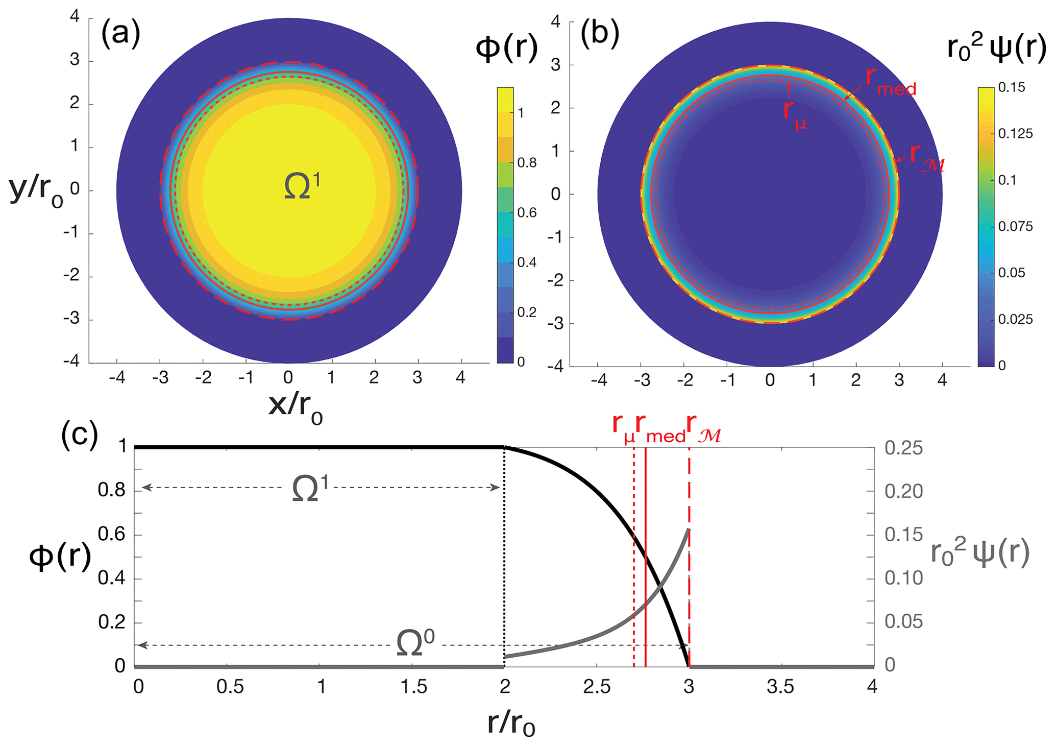
Figure 2(a) PHM and (b) PHDM examples for the freezing viscous gravity current model under a uniform sampling of the freezing rate parameter Γ. (c) One-dimensional profile of the PHM and PHDM with the distribution centers indicated. This example was calculated with $r_N\left({\mathrm{\Gamma }}_{\min }\right)/r_{\mathrm{0}}=\mathrm{2}$ and $r_N\left({\mathrm{\Gamma }}_{\max }\right)/r_{\mathrm{0}}=\mathrm{3}$ or ${\mathrm{\Gamma }}_{\min }/\mathit{\tau }=\mathrm{255}$ and ${\mathrm{\Gamma }}_{\max }/\mathit{\tau }=\mathrm{6560}$.

Download

These relationships lead naturally to the estimates of the center of the distribution (Fig. 2) as defined above,

and the standard deviation,

where

where Eq. () was substituted into Eq. (), and Eqs. (15) and (20) were used to calculate Eq. (34). Higher moments of the distribution are theoretically calculable by repeated integration by parts, from which additional facts may be learned about the distribution.

These calculations can be made analytically because of the ability to write the equation of the boundary and because that equation is invertible for the unknown parameter; that is, it can be written as r_N(Γ) (a boundary in Euclidean space) and as Γ(r_N) (a boundary in parameter space). This example also serves to highlight the asymmetry of the PHM despite the underlying uniform distribution of physical parameters. This asymmetry is highlighted by the significant spread in the mean, median, and modal boundaries (Fig. 2).

This example was greatly simplified by the assumption of radial symmetry, allowing the distribution to be cast onto one random variable, the radius of the flow boundary, giving integral curves of constant azimuthal angle which are linear in map view. However, in most realistic cases, this is a very poor assumption and the distribution will vary between integral curves.

3.2 Example 2: Mohr–Coulomb flow on an inclined plane

To see the full realization of these concepts, a true two-dimensional problem is required. A simple example flow which had been well-studied is a lab-scale granular flow of sand down an inclined plane with a Mohr–Coulomb (MC) friction relation analogous to a natural-scale debris avalanche or landslide (Patra et al., 2005, 2018a, b; Dalbey et al., 2008; Yu et al., 2009; Webb and Bursik, 2016; Aghakhani et al., 2016). In the simulated version, a MC rheology variant of the Saint-Venant shallow water equations is solved numerically with the purpose-built solver TITAN2D (available from https://vhub.org/, Version 4.0.0, VHUB, 2016). In this setup (Fig. 3a), a 5 cm radius, 5 cm high cylindrical pile is placed 0.7 m up a 1 m long, 38.5^∘ inclined plane and is allowed to flow out onto a flat runout 0.5 m long by 0.7 m wide. In accordance with MC theory, the flows were stopped locally when the sum of the drag due to internal and bed friction exceeded the gravitational forces, and the simulations were stopped globally after 1.5 s, when the flow dynamics had typically ceased (Patra et al., 2018b). In this case, the solution variable of interest h is the maximum flow height over time, that is, the maximum flow height that each point experiences through the course of the flow.

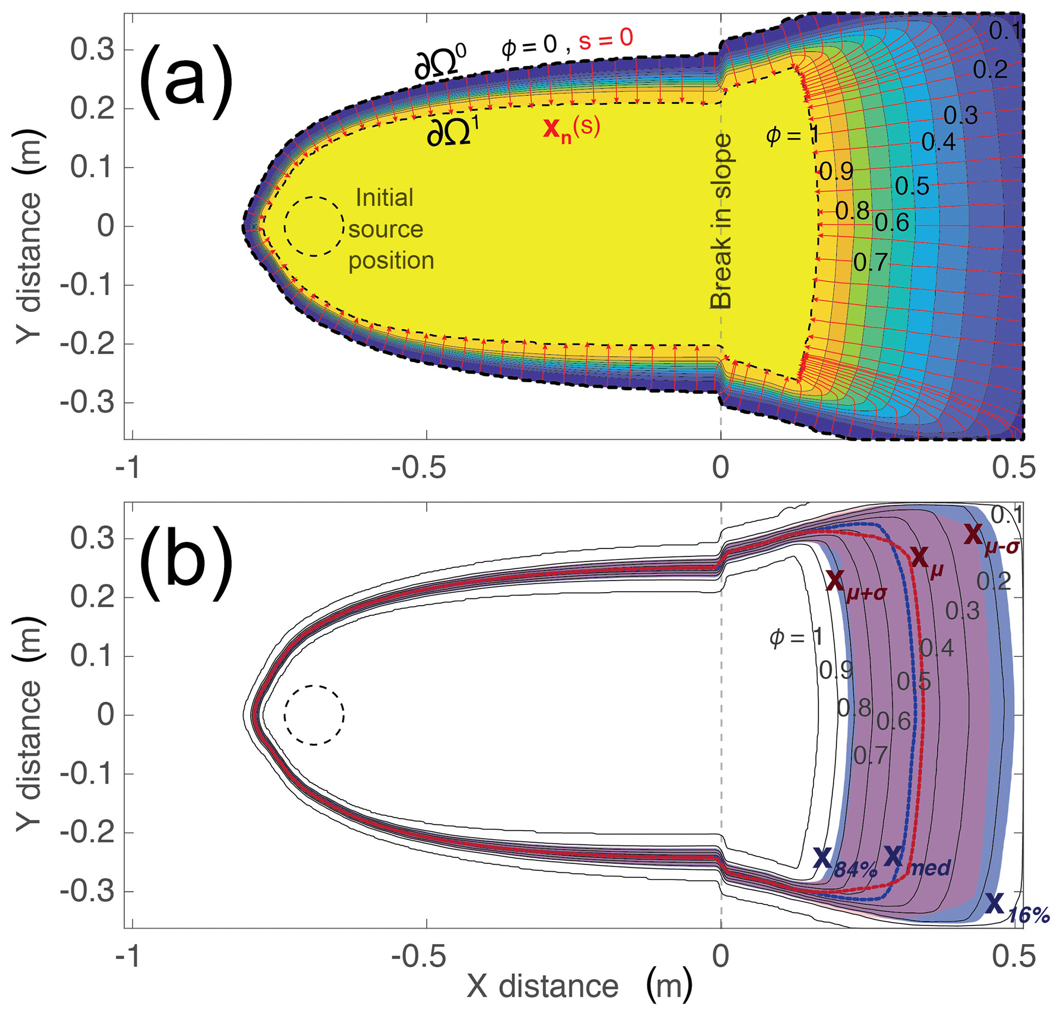
Figure 3(a) PHM contours for a Mohr–Coulomb (MC) flow on an inclined plane with integral curves x_n(s) (red) connecting points on ∂Ω⁰ to points on ∂Ω¹ as defined in the text. (b) Mean (x_μ, red curve) and median (x_med, blue curve) flow boundary sets as well as regions within 1 standard deviation from the mean (red) and containing 68 % of the possible flow boundaries around the median (blue).

Download

The uncertain parameters in the problem for a given granular medium are the internal and basal friction angles of the medium, φ_int and φ_bed respectively. To construct the PHM for this flow, 512 TITAN2D simulations were performed over a Latin-hypercube-sampled input parameter space of

To construct the indicator functions for this experiment, a thickness threshold of h₀=1.0 mm was adopted. The PHM was then computed by averaging the indicator functions: a discrete analogy to Eq. (4). Owing to the discrete nature of the data, all continuous operations on the PHM were done by numerical finite differences and quadrature.

The PHM for this problem has many important characteristics, notably that the greatest dispersion in the probability contours occurs in the runout zone, owing principally to the uncertainty in φ_bed. Additionally, the spreading angle of the flow as a whole experiences a significant increase as the flow passes the break in slope (Fig. 3a). In order to calculate the mean flow boundary set and higher moments of this distribution, the gradient ascent curves of Eq. (5) were integrated numerically from a finite set of closely spaced points around an approximation of ∂Ω⁰ defined as

where J=2049 is the number of such points generated by numerical contouring. Equation (5) was integrated by Euler's method with a 1 mm step forward in s (Δs_k=1 mm), thus fixing $\left|\right|{\mathit{x}}_n^j\left(s_{k+\mathrm{1}}\right)-{\mathit{x}}_n^j\left(s_k\right)\left|\right|=\mathrm{1}$ mm. This yielded discrete integral curves ${\mathit{x}}_n^j\left(s_k\right)$ of varying lengths around the perimeter of the PHM (Fig. 3a). With each ${\mathit{x}}_n^j\left(s_k\right)$ calculated, ϕ(s_k;l^j) was constructed and the parameter μ^j calculated on each curve, yielding an estimate of x_μ(l) by interpolation of the discrete points ${\mathit{x}}_{\mathit{\mu }}^j$ (Fig. 3b). The standard deviations σ^j and the standard deviation space curves x_μ±σ(l) were calculated by similar means (Fig. 3b). An important result of these calculations is that for almost every part of the runout zone, the mean flow boundary set x_μ is dislocated from the median flow boundary set x_med ($\mathit{\varphi }=\frac{\mathrm{1}}{\mathrm{2}}$), indicating qualitatively the general asymmetry of this distribution. Additionally the region bounded by the curves x_μ±σ is remarkably different from the region which bounds the central 68 % of the data – the percent bounded by ±σ in the normal distribution (Fig. 3). All of this indicates that for PHMs of even simple realistic flows, the underlying statistics are not only nonnormal and nonsymmetric, they are variable along the boundary of the hazard.

3.3 Example 3: PHM and PHDM construction from simulations of the 1955 debris flow in Atenquique, Mexico

Following from the previous application of the PHM statistics to a simple flow, here we present a more advanced application: construction and analysis of a PHM for a more complex flow over natural topography. This example consists of numerical modeling detailed in Bevilacqua et al. (2019) of the 1955 volcaniclastic debris flow which destroyed the village of Atenquique at the base of Nevado de Colima, Mexico. On 16 October 1955, at 10:45 LT, residents of Atenquique experienced the arrival of an 8–9 m high debris flow wave front that subsequently destroyed much of the town's buildings and infrastructure and caused more than 23 deaths (Ponce Segura, 1983; Saucedo et al., 2008). The debris flow was initiated by landsliding in the upper reaches of the Atenquique, Arroyo Seco, Los Plátanos, and Tamazula fault ravines, with a minimum initial volume of 3.2×10⁶ m³ (Rupp, 2004; Saucedo et al., 2008). In the simulation of this flow, this volume was increased by 10 %–50 % to give volumes of $V=\mathrm{4.25}\pm \mathrm{0.75}\times {\mathrm{10}}^{\mathrm{6}}$ m³ (Bevilacqua et al., 2019).

We analyze an ensemble of TITAN2D simulations of this flow that were generated by Bevilacqua et al. (2019) using a physically realistic rheology for a debris flow, the Voellmy–Salm (VS) rheology. This rheology is parameterized by a bed friction coefficient μ_VS and a velocity-dependent friction parameter ξ which approximates turbulence-induced dissipation and is uncertain over several orders of magnitude. Consequently, ξ is sampled logarithmically (Patra et al., 2018a, b). The flow was initiated from five source paraboloidal piles of material with unitary aspect ratios and volumes represented as constant fractions of the total flow volume which were proportional to the drainage size (Fig. 4a). The input parameter space ℬ for this simulation was taken as a convex subset of {(arctan (μ_VS), log ₁₀(ξ), V)} with the bounds 1^∘ ≤ arctan (μ_VS)≤ 3^∘, $\mathrm{3}\le {\log }_{\mathrm{10}}\left(\mathit{\xi }\right)\le \mathrm{4}$, and $\mathrm{3.5}\times {\mathrm{10}}^{\mathrm{6}}\le V\le \mathrm{5.0}\times {\mathrm{10}}^{\mathrm{6}}$. This set was determined using information about the known flow runout, flow arrival time in the town, and exclusion of ravine overflow in conjunction with a round of preliminary simulations according to a new procedure of probabilistic modeling setup (Bevilacqua et al., 2019).

Figure 4(a) PHM and (b) PHDM for a lahar inundating Atenquique, Mexico, using the numerical model TITAN2D incorporating the parameter space described in the text. (c) Profiles of the PHM and PHDM across sections X–X^′ and Y–Y^′ highlighting the fact that each side of the PHM profile acts as a CDF for the location of the inundation edge with the corresponding scaled PDF given by the same profile along the PHDM. Grey background (c) indicates regions where ϕ=0 or ϕ=1 (ψ=0).

Download

As in the previous example, the solution variable of interest is the maximum flow height over time; however, here the height threshold h₀=5.0 cm is used. The 350 VS simulation indicator functions were averaged as in the previous example to obtain the PHM for this flow (Fig. 4a). For such a complex flow margin, the gradient-ascending integral curves could not be computed reliably at the resolution of the model; however, the PHDM was calculated using a discrete gradient operation, giving a sense of the maximum likelihood for the inundation boundary (Fig. 4b). Owing to the complexity of this flow and its underlying topography, profiles of the PHM and PHDM across the flow indicate that each margin of the flow is distributed nonsymmetrically, although the sense of asymmetry does not appear to be systematic (Fig. 4c). In numerous locations, the flow boundary distributions (profiles of the PHDM) are multimodal, which are interpreted to be controlled primarily by complexities in the underlying topography, relating to partial spillover of the steep bounding ravines. Of particular interest is the behavior of the PHM and PHDM at the distal margin of the flow in the town of Atenquique and as it leaves town downriver to the south and upriver to the north. To the south (downriver) the PHM decays over a very long distance (>5 km) down a constrained channel, giving small values for the PHDM along the direction of flow (Fig. 4b). Consequently in this region, the flow boundary distributions are multimodal with weaker modes more distally and only the lateral boundaries being well-defined. This portion of the flow highlights some important problems with PHMs in general; they may include regions where the distribution spans a wide range of distances and will therefore have a large standard deviation, yielding high uncertainty in the flow boundary location. The accuracy of the PDFs over the integral curves in this region is most sensitive to the number of samples affecting this region. In a finite sampling of the parameter space, these PDFs may contain spurious peaks in regions where very few models reach. For example if only a small number of models reach a region where the PHM decays over many grid cells, unless some smoothing or interpolation is applied before gradient calculation, the PHM will decay stepwise with many grid spaces between steps. When the numerical gradient is calculated over a set cell size, these steps will become peaks in the PDFs and PHDM. This problem is generally absent where the PHM step size is more comparable to the scale of the grid spacing used by the gradient operator.

This complex example highlights the need for consideration of additional probability measures than simply the probability contours. Where the flow is not narrowly confined or where spillover has occurred, the shape of the distribution becomes relevant and may yield significantly different results than estimating the likely flow boundary as one of the probability contours.

4.1 Analytic models

Although an analytic model (Quick et al., 2017) was invoked in the first example to make an exact calculation of the mean, median, mode, and standard deviation of the flow boundary, the real value of these models is that they are generally invertible and can be used to extract information about the input parameters from the properties of a given flow. Specifically, the PDF measuring the space of input parameters f can be inverted from data collected from the natural phenomena that the analytic model represents. Using the example of the freezing viscous gravity current highlighted above (Quick et al., 2017), we show that an ensemble of natural examples of such flows can be used to invert the PDF of input parameters directly from the definition of the PHM. Suppose that remote sensing or geological field work yields data on the maximum radii (r_N) for an ensemble of these natural freezing gravity currents and that a natural PHM model is constructed called $\widehat{\mathit{\varphi }}\left(r\right)$, which represents the discrete CDF of radii that were measured. As before, we consider a simplified case wherein the most uncertain parameter from among the collection of natural flows is the freezing rate parameter Γ. If the researcher were sufficiently confident that these assumptions and the governing equation (Eq. 21) accurately describe these flows, then the only differences between $\widehat{\mathit{\varphi }}\left(r\right)$ and Eq. () would arise as a consequence of the PDF f(Γ) of the natural input space being nonuniform. Consequently, because the formula for the flow boundary ($r_N\left(\mathrm{\Gamma }\right)=r_{\mathrm{0}}(\mathrm{1}+\mathrm{\Gamma }/\mathit{\tau }{)}^{\mathrm{1}/\mathrm{8}}$) is known and is invertible, the formula for the PHM can also be inverted directly in this simple case as follows:

Applying the fundamental theorem of calculus and the chain rule yields

In practice, the collected data would be in the form of a normalized histogram $\widehat{p}\left(r_N\right)$ for the maximum flow radii. As a discrete approximation, $\widehat{\mathit{\varphi }}\left(r_N\right)$ is the associated complementary CDF for $\widehat{p}$. Consequently, the PDF over parameter space could be written approximately as

where Γ_i are sample points at which the calculation is performed. This illustrates the general fact that the distribution of flow boundaries observed reflects the underlying parameter space PDF weighted by the Jacobian (univariate derivative in this case) of the analytic mapping from parameter space to the flow boundary location in Euclidean space. Generally, unless the analytic model predicts that the boundary of a flow (Ω(β)) is proportional to a given parameter, the input space distribution f(β) undergoes a nonlinear transformation in the construction of a PHM and PHDM. More precisely, we remark that the calculated distribution is the conditional probability density f(Γ|β_k), where β_k represents all of the other parameters that were assumed to be known precisely. Inverting the PHM for the joint parameter space PDF is beyond the scope of this work.

4.2 Numerical models and probabilistic hazard assessment

If the parameter space of a given inundation hazard scenario and a realistic physical model of the process are known, a simple numerical experiment can be run using classical Monte Carlo methods or other Monte Carlo variants as was done for the granular flow on an inclined plane (Patra et al., 2018b) or the 1955 Atenquique lahar (Bevilacqua et al., 2019), as well as even more sophisticated sampling methods (e.g., Bursik et al., 2012, Bayarri et al., 2015). As in the examples in this study, the hazard map and hazard density map and the associated statistics may be generated from such experiments. This may then be used to give additional information to a probabilistic assessment of the hazard rather than merely the inundation probability contours. In this context, the method outlined here is capable of generating the typical measures that would appear in routine statistical analyses of distributions. The most obvious among these is the mean flow boundary and standard deviation region. These are fundamentally newly calculable measures for PHMs and should be included in probabilistic hazard assessments.

As illustrated in the examples, the mean boundary may differ significantly from the median boundary owing to the asymmetric statistics that are inherent to typical nonlinear flows. Furthermore, this asymmetry suggests that the modal or maximum likelihood boundary may be of interest to users of these assessments as well. For the scientific component of probabilistic hazard assessments to have maximum impact and accuracy, these analyses should incorporate the full statistics of the PHM.