the Creative Commons Attribution 4.0 License.
the Creative Commons Attribution 4.0 License.
 | 26 Jul 2019
Effects of horizontal resolution and air–sea flux parameterization on the intensity and structure of simulated Typhoon Haiyan (2013)
Mien-Tze Kueh
Wen-Mei Chen
Yang-Fan Sheng
Simon C. Lin
Tso-Ren Wu
Eric Yen
Yu-Lin Tsai
This study investigates the effects of horizontal resolution and surface flux formulas on typhoon intensity and structure simulations through the case study of the Super Typhoon Haiyan (2013). Three sets of surface flux formulas in the Weather Research and Forecasting Model were tested using grid spacings of 1, 3, and 6 km. Increased resolution and more reasonable surface flux formulas can both improve typhoon intensity simulation, but their effects on storm structures differ. A combination of a decrease in momentum transfer coefficient and an increase in enthalpy transfer coefficients has greater potential to yield a stronger storm. This positive effect of more reasonable surface flux formulas can be efficiently enhanced when the grid spacing is appropriately reduced to yield an intense and contracted eyewall structure. As the resolution increases, the eyewall becomes more upright and contracts inward. The size of updraft cores in the eyewall shrinks, and the region of downdraft increases; both updraft and downdraft become more intense. As a result, the enhanced convective cores within the eyewall are driven by more intense updrafts within a rather small fraction of the spatial area. This contraction of the eyewall is associated with an upper-level warming process, which may be partly attributed to air detrained from the intense convective cores. This resolution dependence of spatial scale of updrafts is related to the model effective resolution as determined by grid spacing.
- Article
(4483 KB) - Full-text XML
-
Supplement
(226 KB) - BibTeX
- EndNote


Intensity forecasting of tropical cyclones (TCs) remains a major challenge to numerical weather prediction. Numerous small-scale processes are involved in TC development, most of which are parameterized in numerical weather models. Therefore, the accuracy of physical representations in numerical models is crucial to TC intensity prediction (e.g., Bao et al., 2012). By contrast, several studies have shown that increasing the horizontal resolution has a positive effect on TC intensity and structure simulation (e.g., Davis et al., 2008; Fierro et al., 2009; Nolan et al., 2009; Gentry and Lackmann, 2010; Kanada and Wada, 2016). Of these, most have recognized that sufficiently high resolution is responsible for development of deep and intense eyewall updraft and thus a more organized inner-core structure of TCs (Fierro et al., 2009; Nolan et al., 2009; Gentry and Lackmann, 2010; Gopalakrishnan et al., 2011; Kanada and Wada, 2016). However, even with a very high model resolution, physical processes remain a source of uncertainty in numerical weather prediction of TC intensity (e.g., Fierro et al., 2009; Gentry and Lackmann, 2010). For instance, the predictions of TC intensity and structure are sensitive to the model representation of physical processes involving planetary boundary layer evolutions (Braun and Tao, 2000; Hill and Lackmann, 2009; Bao et al., 2012; Nolan et al., 2009; Kanada et al., 2012; Coronel et al., 2016) and surface exchange fluxes (Braun and Tao, 2000; Davis et al., 2008; Hill and Lackmann, 2009; Bao et al., 2012; Nolan et al., 2009; Chen et al., 2010; Green and Zhang, 2013; Zhao et al., 2017).
Gopalakrishnan et al. (2011) noted that, at higher resolutions, larger moisture fluxes (resulting from strong convergence in the boundary layer) can lead to stronger storms. Kanada et al. (2012) indicated that large heat and water vapor transfers essential for producing intense TCs are attributable to the large vertical eddy diffusivities in lower boundary layers. Nolan et al. (2009) studied the sensitivity of TC inner-core structures to planetary boundary layer (PBL) parameterizations. They found that improvement of the representation of surface fluxes in association with these PBL schemes could improve their respective simulations of the TC boundary layer structure; however, discrepancies between the PBL schemes remained. By conducting 2 km resolution experiments, Coronel et al. (2016) found that both surface drag and vertical mixing in the boundary layer were capable of substantially changing low-level wind structures. The authors further revealed that the mechanisms underlying the two effects differed. Braun and Tao (2000) studied the sensitivity of TC intensity to PBL schemes and surface flux representations using a set of 4 km resolution experiments. They concluded that representation of surface heat fluxes was the most determinative factor in TC intensity simulation. Bao et al. (2012) indicated that different PBL schemes lead to differences in the structure of simulated TC, whereas the near-surface drag coefficient controls the relationship between the maximum wind speed and minimum central pressure.
The air–sea surface flux exchanges of moist enthalpy (through surface latent heat and sensible heat fluxes) act as the primary energy source, whereas the surface momentum flux (the surface drag) is the sink of TC development. The potential intensity for a steady-state (or mature) tropical cyclone has long been hypothesized to be proportional to the ratio of surface bulk transfer coefficients for enthalpy and momentum, CK∕CD (Emanuel, 1986, 1995). The importance of surface flux formulas to TC intensity and structure simulations has also been recognized by numerous studies (e.g., Braun and Tao 2000; Davis et al., 2008; Hill and Lackmann, 2009; Bao et al., 2012; Nolan et al., 2009; Chen et al., 2010; Green and Zhang, 2013). In recent years, observational estimates of surface fluxes revealed that the momentum transfer coefficient exhibits a steady increase to a wind speed of approximately 30 m s−1 but then levels off for higher wind speeds (e.g., Powell et al., 2003; Jarosz et al., 2007; French et al., 2007). For extremely high wind speeds (e.g., exceeding 50 m s−1), observational estimates for the momentum transfer coefficient are rather scattered (Bell et al., 2012; Richter et al., 2016). Both near-surface wind speed and surface sea state are the contributing factors in the formulation of the bulk transfer coefficient for surface fluxes (e.g., Geernaert et al., 1987; Smith, 1988; Fairall et al., 2003; Zweers et al., 2010). Some studies have introduced wind wave information into the momentum flux parameterization (e.g., Fairall et al., 2003; Zweers et al., 2010; Zhao et al., 2017). Zweers et al. (2010) show that their sea-spray-dependent surface drag coefficient is in good agreement with observational estimates reported by Powell et al. (2003) and leads to an improvement in TC intensity forecasts. However, there remains considerable uncertainty in the estimates of these parameters. For example, Green and Zhang (2013) performed the intensity simulation for Hurricane Katrina (2005) by using wind-dependent flux exchange coefficients, and all their experiments overestimated the storm intensity. They attributed this to the lack of an ocean cooling effect in their atmosphere-only model simulations. Zhao et al. (2017) considered three physical processes, namely breaking-wave-induced sea spray, non-breaking-wave-induced vertical mixing, and rainfall-induced sea surface cooling, using a fully coupled atmosphere–ocean–wave model to improve the tropical cyclone intensity simulation. Compared with the observations, their simulations produced a comparable intensity for Super Typhoon Haiyan (2013) but severely overestimated the intensity of another weaker typhoon. It appears that there is still a lack of a surface flux parameterization appropriate for the full spectrum of TC intensity. There is also a need for further study of the interrelationship between surface fluxes and other model configurations, including cloud microphysics as well as grid spacing. For example, the effect of grid spacing on surface flux parameterization regarding TC structure and intensity simulation has not yet been explored.
In this paper, we investigate the effects of model horizontal resolution and surface flux formulas on TC structure and intensity simulations. We intend to study the sensitivity of TC intensity simulations to surface flux parameterizations when model resolution approaches the convective scale. The sensitivity experiments are performed on Super Typhoon Haiyan (2013) with various resolutions and surface flux formulas. Typhoon Haiyan, the strongest TC in 2013, was a category-5-equivalent super typhoon on the Saffir–Simpson hurricane wind scale. Because of its minimum central pressure of 895 hPa, Haiyan became the strongest TC at landfall to date in the western North Pacific Ocean (Schiermeier, 2013; Lander et al., 2014). Lin et al. (2014) suggested that Haiyan's intensity can be considered a league higher than the majority of existing category 5 typhoons on the Saffir–Simpson wind scale. Such super typhoons are expected to increase both in number and intensity under climate change (e.g., Bender et al., 2010; Schiermeier, 2010; Kanada et al., 2012; Lin et al., 2014), which brings even more challenges to TC prediction. Super Typhoon Haiyan (2013) moved west-northwestward over the warm ocean and reached its central pressure of 895 hPa several hours before it made its first landfall. The nonrecurved track tendency allows us to focus on the intensity simulation. Section 2 describes the experimental setup, including the description of the surface flux formulas and experimental designs. Sections 3 and 4 present the results in terms of temporal evolution and radius–height structure, respectively. Section 5 provides statistical and energy spectral analyses, followed by conclusions in Sect. 6.
In this study, the Weather Research and Forecasting Model (WRF)–Advanced Research WRF (ARW) modeling system (version 3.8.1; hereafter, WRF-ARW) was used (Skamarock et al., 2008). In all simulations, all physics options other than the surface flux options (described below) were identical, including the WRF single-moment three-class microphysics scheme (Hong et al., 2004), updated Kain–Fritsch scheme (Kain and Fritsch, 1990; Kain, 2004) with a moisture-advection-based trigger function (Ma and Tan, 2009), Rapid Radiative Transfer Model for Global Circulation Models (RRTMG) shortwave and longwave schemes (Iacono et al., 2008), Yonsei University boundary layer scheme (Hong et al., 2006 for YSU) used with the revised fifth-generation Pennsylvania State University–National Center for Atmospheric Research Mesoscale Model (MM5) similarity surface layer scheme (Jiménez et al., 2012), and the unified Noah land surface model (Tewari et al., 2004) over land. In WRF, the bulk transfer coefficients as well as all surface fluxes (momentum, sensible heat, and latent heat) are parameterized in a surface layer scheme. A brief description of the surface flux parameterization in WRF is provided in Appendix A for reference.
2.1 Flux parameterization in WRF-ARW
The behaviors of bulk transfer coefficients are strongly dependent on the momentum and scalar (heat and moisture) roughness lengths (see Eqs. A7, A8, and A9). Over the ocean, roughness length depends on the varying surface sea state, which is considerably ascribed by wind waves (e.g., Geernaert et al., 1987; Smith, 1988; Fairall et al., 2003). Under high-wind conditions, wave breaking and wind tearing the breaking wave chest generate sea foam and sea spray, thereby leading to significant regime change in the surface sea state, which in turn affects the specification of the roughness length (e.g., Powell et al., 2003; Donelan et al., 2004; Zweers et al., 2010). For the surface layer physics over the ocean, WRF-ARW provides alternative formulations of aerodynamic roughness lengths of the surface momentum and scalar fields for tropical storm application, which can be set through the namelist variable isftcflx. There are three isftcflx options available in WRF-ARW. Here, we study the resolution dependence of all three. Each flux option is referred to by its corresponding number (0, 1, and 2) in the WRF namelist file.
Subsequently, we describe the three sets of formulas of roughness lengths for momentum, sensible heat, and latent heat that have been implemented in the revised MM5 scheme in WRF-ARW. For clarity, we calculated the bulk transfer coefficients and the momentum scaling parameter (friction velocity) with respect to the three sets of implemented roughness length formulas in the case of neutral stability and a reference height of 10 m, using a set of pseudo-wind speeds. Under neutral condition, the stability parameters and are zero (see Eqs. A7, A8, and A9); therefore, all terms that involving the stability function can be dropped. The results are depicted in Figs. 1 and 2.
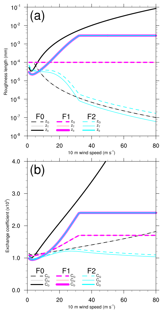
Figure 1Plots of (a) roughness lengths and (b) bulk transfer coefficients versus wind speed at 10 m height for neutral conditions. Flux schemes F0, F1, and F2 are colored black and gray, red and pink, and green. The thick solid curves are z0 and CD, thin solid curves are zh and CH, and dashed curves are zq and CQ. It is noted that some curves are identical. For F1 and F2, z0 (and thus CD) is the same; for F1 and F2 the respective heat and moisture roughness and coefficients are the same: zh=zq and CH=CQ.
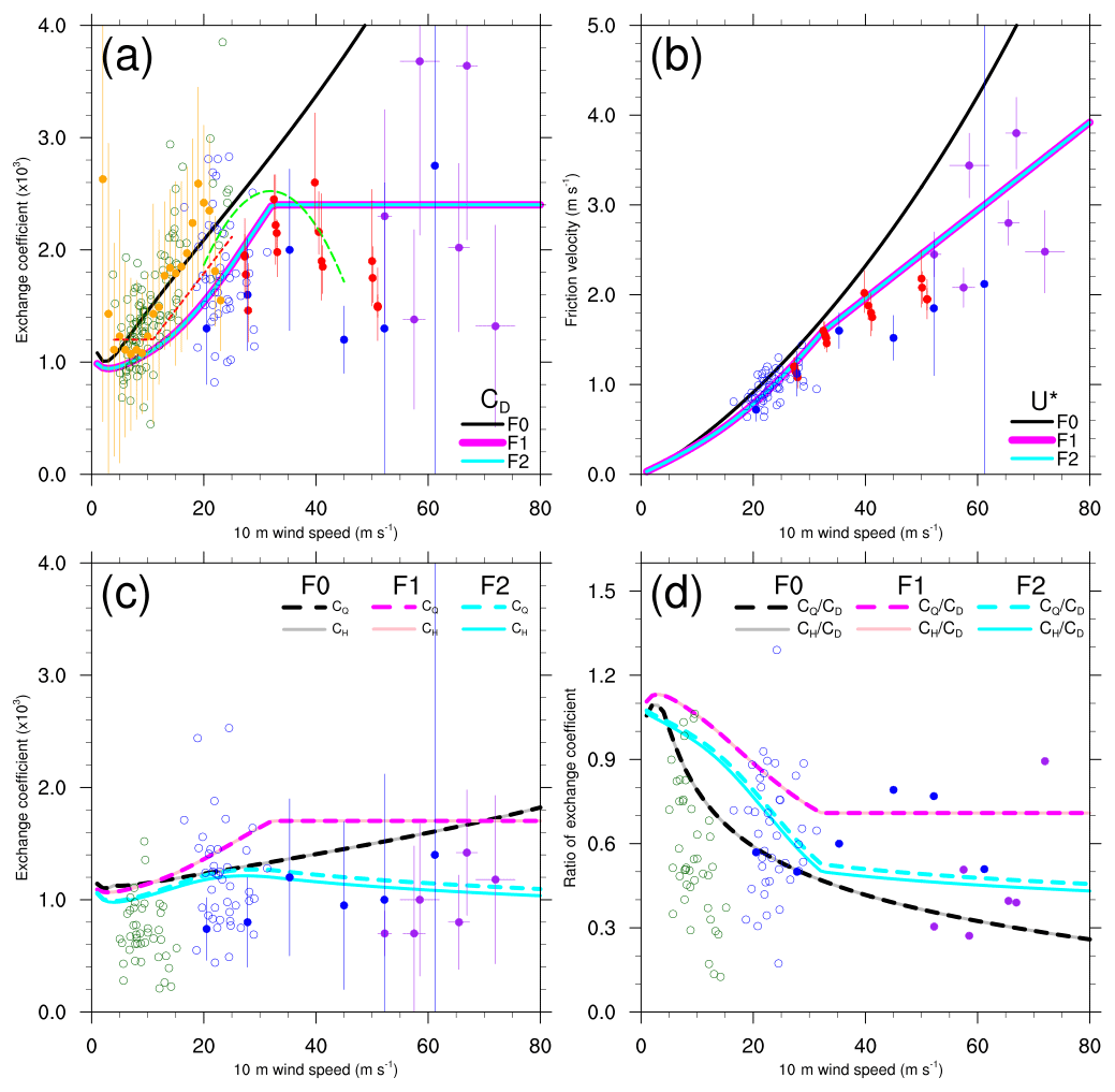
Figure 2Plots of (a) momentum transfer coefficients, (b) friction velocity, (c) scalar transfer coefficients, and (d) transfer coefficient ratios versus wind speed at 10 m height from available observational estimates as found in the literature. The scalar transfer coefficients shown here can be CH, CQ, or CK upon the availability in the literature that we referred to in this study. The purple dots represent the values from Bell et al. (2012), blue circles represent values from French et al. (2007), dark green circles represent values from Geernaert et al. (1987), green curve represents values from Jarosz et al. (2007), red curve represents values from Large and Pond (1981), red dots represent values from Powell et al. (2003), blue dots represent values from Richter et al. (2016), and the orange dots represent values from Vickers et al. (2013). The curves are given by fitted equations; the circles represent the available data points; the dots represent average values in a range of wind speed bins with the bars showing the corresponding data spread as denoted by either the standard deviations or the 95 % confidence intervals, where the wind speed bin and the representation of data spread vary in the literature. Table B1 provides brief information of these observational estimates. The respective bulk parameters derived from WRF, represented as shown in Fig. 1, are superimposed for a comparison.
2.1.1 Momentum and moisture roughness length for flux option F0
For the default flux option (F0), the momentum roughness length is given as Charnock's (1955) expression plus a viscous term, following Smith (1988):
where α is the Charnock coefficient and v the kinematic viscosity of dry air, for which a constant value of m2 s−1 is used. The Charnock expression relates the aerodynamic roughness length to friction velocity for describing the gross effect of wavy sea surface, which is generated and supported by wind stress; the viscous term describes roughness behavior under smooth flow conditions. The use of this roughness length formula yields a monotonic increase in the momentum transfer coefficient, as well as roughness length, with wind speed exceeding approximately 3.0 m s−1 (Fig. 1; black thick solid curve). A constant value of α=0.0185 is used for F0.
The moisture roughness length is adapted from COARE 3.0 (Fairall et al., 2003) and expressed as a function of the roughness Reynolds number, with an additional lower limit of used in this option:
where is the roughness Reynolds number and v the kinematic viscosity of dry air and a function of air temperature for the R∗ calculation. The temperature roughness length zh is set to equal to zq. The upper limit of keeps the scalar roughness length invariant at extreme wind speeds (below approximately 4.0 m s−1), whereas the lower limit of is implemented to prevent the model from blowing up. Below this high wind speed, the heat and moisture transfer coefficients increase monotonically with wind speed (Fig. 1; gray thin solid and black dashed curves). For this option, the formulas of roughness lengths are different from that used by Green and Zhang (2013), where the viscous term for z0 was given as a constant value of , zh is set equal to z0, and zq is set to a somewhat different functional form of z0 and u∗.
2.1.2 Momentum and moisture roughness length for flux option F1
For the flux option 1 (F1), the momentum roughness length is expressed as a blend of two roughness length formulas (Green and Zhang, 2013):
where the first roughness length formula (z1) is again the Charnock (1955) expression plus a constant value of the viscous term, with α=0.011, as suggested by Smith (1988). The second formula (z2) is the exponential expression from Davis et al. (2008) plus a viscous term; here a constant kinematic viscosity m2 s−1 is used. The two roughness length formulas are combined using a weight function (zw), with a lower and upper limit on z0 of m and m, respectively. The lower and upper limits on z0 are adapted from Davis et al. (2008), with a slightly different value of the lower limit. The upper limit used here acts to prevent a monotonic increase in the momentum roughness length as well as the momentum transfer coefficient, under high-wind conditions. The resulting curves present an increase with wind speed below 33.0 m s−1 but exhibit a leveling-off behavior starting at the wind speed of 33.0 m s−1 (Fig. 1; red thick solid curves). The wind speed of 33 m s−1 is extremely close to the lower limit of maximum wind speed for a typhoon. The use of this z0 formula results in apparently smaller momentum roughness length and transfer coefficient at all wind speeds than that in F0. This leveling-off in CD with wind speed suggests a decline in the efficiency of the exchange of momentum across the air–sea interface (see Eq. A1). Considering that the drag effect acts as a momentum sink in the surface layer, it is expected that an atmospheric simulation using the z0 formula of F1 shall retain a larger portion of the total amount of near-surface momentum at all wind speeds than that using the F0 formula, and such a difference in the transfer efficiency becomes increasingly significant with higher wind speeds because of the leveling-off behavior seen in F1.
F1 sets m for all wind speeds. Large and Pond (1982) suggested constant values for zh and zq under different conditions of stability, ranging from 10−9 m (stable) to 10−4 m (unstable). The constant value of 10−4 m used here corresponds roughly to the unstable condition in Large and Pond (1982). While using an invariant scalar roughness length, the heat and moisture transfer coefficients can still vary with wind speed (Fig. 1; pink thin solid and red dashed curves) because of the drag-dependent effect (see Eqs. A7, A8, and A9). Consequently, the heat and moisture transfer coefficients are also beginning to level off at the wind speed of 33.0 m s−1.
2.1.3 Momentum and moisture roughness length for flux option F2
For the flux option 2 (F2), the momentum roughness length is the same as that for F1. The temperature and moisture roughness lengths are expressed based on the formula proposed by Brutsaert (1975a):
where R∗ is the roughness Reynolds number, κ is the von Karman constant, Pr and Sc are the Prandtl and Schmidt numbers, and 7.3 and 5 are experimental constants (Brutsaert, 1975b). As in F0, a temperature-dependent v is also used for R∗ calculation. The values of κ, Pr, and Sc are set to 0.40, 0.71, and 0.60, respectively, as suggested by Brutsaert (1979). This set of formulas relates the heat and moisture roughness length to a scaling of z0 by exponential expression, where the exponent contains information about the near-surface flow regime as characterized by the roughness Reynolds number and Prandtl and Schmidt numbers. The resulting zh and zq are practically an exponential decay of z0 with wind speed (Fig. 1; green thin solid and green dashed curves). The scalar roughness lengths in F0 and F2 both decrease with wind speed, and their decreasing rates as well as magnitudes are similar at higher wind speeds. However, their resulting scalar transfer coefficients are apparently different. Unlike the monotonic increasing behavior found in F0, for F2 the heat and moisture transfer coefficients show an upward trend with wind speeds below 33.0 m s−1 and then start decreasing at this wind speed. Such a discrepancy between F2 and F0 results from the drag-dependent effect in the scalar transfer coefficients (see Eqs. A7, A8, and A9).
2.2 Comparison between modeled and observational bulk transfer coefficients
Figure 2 presents the bulk transfer coefficients and friction velocity obtained from existing observational estimates as found in the literature. A brief description of these observational estimates is provided in Appendix B. Overall, the behavior of CD in F1 and F2 as a function of wind speed is more consistent with recent observations than that in F0 (Fig. 2a). Under the low- to moderate-wind conditions, all the flux options generally predict similar behaviors to those observed in the observational estimates, and their values are within the observed data range. For the higher wind conditions, F1 and F2 predict a leveling-off in CD values with wind speed such that it is significantly different from F0 starting at 33 m s−1. Considering the large discrepancy as well as the large spread of data found in the observational estimates beyond the wind speeds of approximately 55 m s−1, the leveling-off behavior of CD values in F1 (and thus F2) is more reasonable than the monotonic increasing CD values in F0 (Fig. 2a). This is also supported by the comparison of the variations in friction velocity (Fig. 2b).
In Fig. 2 c, we plotted all observational estimates of scalar transfer coefficients (CH, CQ, and CK) available in the literature that we referred to for this study (Table B1). Visually, we see an upward trend between the data samples from Geernaert et al. (1987) and French et al. (2007) but no significant trend between French et al. (2007) and the remaining two with higher-wind conditions (Bell et al., 2012; Richter et al., 2016). However, Geernaert et al. (1987) reported that their data were mostly collected under stable conditions. Studies have revealed a stability dependence of CH, in which values of CH under stable conditions are lower than those under unstable conditions (Large and Pond, 1982; Smith, 1988). Accordingly, the applicability of the increases in CH and CQ with wind speed remains elusive. Compared with F0, both F1 and F2 give a relatively reasonable pattern of CH and CQ, with F2 fitting the observational estimates better than F1 does.
In the context of the leveling-off behavior of CD at high wind speeds as well as the absence of a monotonic increase in CH and CQ with wind speed, both F1 and F2 provide more reasonable formulas for parameterizing the surface fluxes than F0. Furthermore, F1 predicts larger CH and CQ at all wind speeds than F2 does, implying that F1 could gain larger enthalpy fluxes. Because the formula of z0 (and thus CD) is identical in F1 and F2 while their respective formulas for zh and zq are different, and because the behaviors of transfer coefficients in F0 are quite distinct from those in F1 and F2, we use the CK∕CD ratio to compare between the three flux options. By assuming that here, we plot the ratios CH∕CD and CQ∕CD in Fig. 2d. All the flux options present a decrease in the ratio with wind speed, except that for F1 an upward trend and leveling-off pattern are found under extremely low wind and high wind conditions, respectively. The CK∕CD derived from the available observational estimates was also superimposed for reference. We noted that for moderate to high wind speeds, the values of CK∕CD are all below the lower limit, namely 0.75, for mature hurricanes as suggested by Emanuel (1995). Even for F1, the ratio levels off at a value of 0.7. Relatively small value of CK∕CD, compared with the lower limit of 0.75, is indeed not uncommon and has been reported by numerous studies based on observational measurements (e.g., Drennan et al., 2007; Zhang et al., 2008; Bell et al. 2012) and numerical simulations (e.g., Hill and Lackmann, 2009; Green and Zhang, 2013). Nonetheless, we still can qualitatively relate the tropical cyclone intensity to the ratio of CK∕CD. Accordingly, F1 is expected to have the highest potential to achieve the most intense storm among the three options because it has the highest values of CK∕CD almost at all wind speeds. F0 has the lowest values of CK∕CD owing to its largest values of CD, thereby having the lowest potential to produce a comparable storm intensity to F1.
2.3 Experimental designs
Table 1 summarizes the experiments designed for this study. There were three resolution groups, with horizontal grid spacing of 1, 3, and 6 km. All three isftcflx surface flux options were tested for these three resolution groups. We considered 3kmF0 as the control experiment. All experiments used a single domain and 45 vertical levels. The model domain covered a spatial region bounded by 0–19.62∘ N latitudes and 117.88–147.12∘ E longitudes (Fig. 3; red box). The experiment procedure included a nudging and a sensitivity stage. For the nudging stage, the grid nudging (Staufer and Seaman, 1994) implemented in WRF was applied to each resolution group using the default flux option (F0). The numerical solutions were nudging toward the gridded reanalysis for 24 h starting at 00:00 UTC on 4 November 2013 (Fig. 3; tan dots). In this study, the analysis nudging was applied to the horizontal wind components, potential temperature, and water vapor mixing ratio. The nudging coefficients for all variables were set at 0.0003 s−1. Nudging was only applied at all levels above the PBL to allow for the development of mesoscale processes near the surface. The National Centers for Environmental Prediction Global Forecast System (GFS; Environmental Modeling Center 2003, 2016) operational global analysis dataset was used to provide the initial and boundary conditions. The GFS global analysis has a horizontal resolution of 0.5∘, and it is also used as data for the grid nudging. The model sea surface temperatures (SSTs) were taken from the RTG-SST dataset (Gemmill et al., 2007), with daily time resolution; there was no ocean feedback in this study. The SSTs varied during the nudging stage up until 00:00 UTC on 5 November 2013 and thereafter remained fixed throughout the sensitivity simulation such that the differences in underlying SSTs between the flux options became negligible. Consequently, sensitivity of typhoon intensity and structure to the flux options (thus the surface flux formulas) can be determined to a large extent. All the sensitivity experiments started at 00:00 UTC on 5 November 2013 and ended at 06:00 UTC on 8 November 2013 (Fig. 3; red dots). All results are from within the 78 h that the experiments ran for.

Figure 3The model domain (red box) and calculation domains for the contoured frequency by altitude diagrams (blue box) and for energy spectra (cyan box). The red, tan, and green and dots represent the locations of Haiyan obtained from the best-track dataset. The red dots indicate the period of sensitivity experiments, the tan dots indicate the nudging period, and the green dots are the locations outside our simulation period.
Table 1Summary of the resolutions and surface flux options tested. The nudging period for all experiments is between 00:00 UTC on 4 November 2013 and 00:00 UTC on 5 November 2013, with an identical nudging setting for each resolution group using the default flux option (F0). Thereby the corresponding sensitivity experiments start with an identical initial TC (tropical cyclone) structure and location. The MCP and MSW indicate, respectively, the minimum central pressure at the TC center and maximum surface wind speed near the TC center.

Typhoon Haiyan formed in the western North Pacific on 3 November 2013 and underwent a rapid intensification a few days later. Haiyan reached peak intensity of 895 hPa before it made a cataclysmic landfall near Guiuan, Eastern Samar, Philippines, on 8 November 2013 at about 04:40 PHT (UTC + 8). The storm then crossed the Philippines, migrated west-northwestward, and made its final landfall in Vietnam. Our simulation period for the sensitivity experiments covers the stages of Haiyan's peak intensity and landfall. We focus on the mature stage of Haiyan before its landfall near Guiuan, Eastern Samar.
All simulations show a similar west-northwestward movement toward land and appropriately follow the observed best track, but with slower translation speeds (Fig. 4a). The typhoon landfall at Samar island is delayed between 3 and 5 h in these sensitivity simulations. Because of the delayed landfall, we compare the evolution of the typhoon related to its longitudinal position (Fig. 4b). In general, the simulations continue to intensify and reach their peak right after 18:00 UTC on 7 November 2013 and before landfall. We refer to the time span from 18:00 UTC on 7 November 2013 to 00:00 UTC on 8 November 2013 as the mature stage of the simulated typhoon. In this study, the cumulus parameterization was used for all resolutions. This is because we intend to keep consistency among all cases. Results from an additional simulation of the 1kmF0 with the cumulus parameterization turned off revealed that the simulated Haiyan intensity and structure are overall similar. The minimum central pressure and storm track of the 1kmF0 without cumulus parameterization follow almost the same evolution as that of 1kmF0 (Fig. S3). In our case, the use of a cumulus parameterization in high-resolution (1 km) simulation does not exert considerable influence on the typhoon intensity, track, and structure. Some studies have also revealed that the activation of cumulus parameterization for simulation with grid spacings of 2–3 km produced an overall similar simulated storm to the simulation with explicit convection (e.g., Yu et al. 2011; Li et al. 2018; On et al. 2018).

Figure 4(a) Haiyan's best track (black dots) and simulated tracks of 1 km (blue lines), 3 km (red lines), and 6 km (green lines) from 00:00 UTC on 5 November 2013 through 06:00 UTC on 8 November 2013. Thick and thin curves represent a span of 24 h alternately. (b) The evolutions of the best track and simulated minimum central pressures (hPa) shown in relation to longitude. The longitudinal position of the first landfall of Haiyan is around 125∘ E. The gray circle on each curve denotes the corresponding data point at 18:00 UTC on 7 November 2013. (c) Scatterplot of maximum wind speed versus minimum central pressure. Reference curves Koba and AH_KZ are the operational WPRs for the JMA and JTWC, respectively. Koba_1min is the modified Koba curve with 10 min sustained winds converted to 1 min averaged values. The detailed tracks and central positions of the simulated storms during their mature stage are given in Figs. S1 and S2 in the Supplement.
For each resolution group, F1 is the most intense in terms of minimum central pressure, whereas the intensity of F2 is somewhat between that of F0 and of F1. The intensity is sensitive to model resolution. Overall, the intensity increases as the resolution is changed from 6 to 3 km, but it significantly increases as grid spacing is reduced to 1 km. The experiment 3kmF1 yields an intensity level comparable with that of 1kmF0, demonstrating the benefit of using a more reasonable flux option in improving intensity simulation. Accordingly, the combination of the decrease in the momentum transfer coefficient (generally tends to reduce the energy loss) and increase in enthalpy transfer coefficients (thus more energy gain) has greater potential to yield a stronger storm. Finally, a higher resolution is more conducive to the intensification due to the change in flux formulas.
The comparison between the simulated maximum winds near the typhoon center and the best-track wind information is somewhat complicated owing to the wind speed averaging period (Kueh, 2012; Knapp et al., 2013). We use the International Best Track Archive for Climate Stewardship (IBTrACS) dataset for comparison, which compiles best-track information from various agencies worldwide (Knapp et al., 2010). The best-track information in Figs. 3 and 4a is taken from the WMO subset of the IBTrACS (IBTrACS-WMO, v03r09). The WMO best track for Haiyan is taken from the best-track data provided by the Japan Meteorological Agency (JMA), which relies on a wind pressure relationship (WPR) where the maximum wind is given in terms of 10 min sustained winds (Koba et al., 1991). However, simulated maximum winds near the typhoon center were derived from WRF hourly output instantaneous maximum 10 m wind speeds at the beginning of each hour. Figure 4c presents the scatterplot of maximum wind speed versus minimum central pressure. The discrepancy found between the simulations and the best-track data may be partially due to different wind speed averaging periods. The WMO best-track wind pressure distribution appropriately follows the operational WPR, namely the reference curve Koba. We use a factor of 0.88, which is used operationally at the Joint Typhoon Warning Center (JTWC), to convert the 10 min sustained wind in Koba's WPR to an equivalent 1 min sustained wind. The modified Koba curve Koba_1min now agrees with the operational WPR used at the JTWC. The JTWC's WPR uses 1 min sustained winds (Atkinson and Holliday, 1977; Knaff and Zehr, 2007). In practice, operational WPRs were derived statistically to best fit a set of observed parameters (pressures and winds) by using the gradient wind approximation as a fundamental guide. In the context of statistical regression and use of observed parameters, other information, such as the vortex size, ambient conditions, and geographical location, would be incorporated into these reference curves (Knaff and Zehr, 2007). The operational WPR may somewhat be considered the best fit to the actual mass–wind relation of TCs. The winds and pressures of Haiyan from the JTWC best-track data have been plotted in Fig. 4c, and the distribution agrees well with the JTWC operational WPR; we thereby omitted them from the plot. All our simulated wind pressure distributions present similar slopes to the two reference curves of 1 min averaged winds, indicating that these simulations are valid for further investigation of the typhoon structures.
Bao et al. (2012) reported that the simulated WPR is controlled by the formulation of the drag coefficient. From a set of simulations for North Atlantic TCs between 2008 and 2011, Green and Zhang (2013) found that different CD formulas affect wind pressure distribution (see Fig. 9 in Green and Zhang, 2013). We found insufficient evidence supporting any apparent slope change in wind pressure distributions of different flux options. This discrepancy may be partially due to the use of the square of the maximum 10 m wind speed in their wind pressure distribution plot. By comparing the respective linear regression curves between all experiments, we found that the differences in flux options and resolution result in a slight change in the slope (data not shown). However, no distinct dependence of the slopes on the choice of flux option and resolution could be identified. In our study, the differences in the wind pressure distribution between these sensitivity simulations are demonstrated by their magnitudes. For each resolution group, F1 is the most intense in terms of both minimum central pressures and maximum winds, whereas the intensity of F2 is somewhat between that of F0 and F1. A comparison of resolution groups used in F0 reveals a significant increase in intensity at higher resolutions during the mature stage (where the storm has a higher strength), with 1kmF0 receiving larger increments. The set of experiments using F1 presents a similar pattern, with the larger increments in 1kmF1 being much more marked.
In brief, increased resolution and more reasonable flux parameterization (e.g., F1 in this case) can both improve typhoon intensity simulation to a certain extent. However, a sufficiently high resolution is more likely to the benefit from improved flux formulas. The implication is 2-fold. First, the use of reasonable flux formulas to improve intensity simulation is perhaps more efficient than using an extremely high resolution when computational resources are limited. Second, higher model resolution is conducive to improving surface flux representation in strong typhoon intensity simulations. The mechanisms underlying these two issues are notable. We address the issue of higher model resolution and its effect on surface flux representation in the following sections.
The sensitivity of simulated typhoon intensity to various resolutions and flux options is also associated with changes in the simulated typhoon structure. To isolate differences between simulations of different grid spacing, the hourly outputs on the WRF native grid were transformed to the cylindrical (polar-height) coordinate system centered at the simulated typhoon at each time point. To avoid spatial sampling issues in the comparison of mass and wind fields, all model outputs were transformed to an identical resolution setting. We used a 3 km horizontal resolution and an uneven vertical resolution with smaller spacing in the boundary layer for the cylindrical transformation. Specifically, the cylindrical coordinate used in this study has an azimuthal resolution of 2∘, a radial resolution of 3 km, and an uneven vertical resolution within the radius and height of 900 and 18 km, respectively. All the data to be analyzed are interpolated from the model native coordinate to the cylindrical coordinate using bilinear interpolation. The zonal and meridional components of horizontal wind fields are transformed to tangential and radial wind components using their standard formulas. The (height-invariant) typhoon center is defined as minimum central pressure using the surface pressure field. We also examined the geometric center for the local minimum pressure and found that the distances between the center at grid point and the geometric center are less that the half of the grid spacing, for the simulation period after 24 h (valid at 00:00 UTC on 6 November 2013). The magnitudes of the vertical tilt of the center (in terms of the WRF output perturbation pressure field) are also small: about the size of one grid box. In this study, radial variations of model fields were all derived from these transformed subsets.
Figure 5 shows the horizontal distributions of wind speed at 10 m height, total rainfall, and surface enthalpy fluxes for F0 with 3 km resolution after the cylindrical transformation. The wind speed distribution shows a ring of higher wind speed (exceeding approximately 42 m s−1), with wider regions of high wind speed over the right side (northern semicircle) of the track, with a partial ring of the maximum wind speed (∼50 m s−1), open to the west, at the range of radii 40–50 km. A region of intense rainfall is located on the left-rear side of the track. Regions of a larger amount of surface fluxes are located near the local maximum wind speeds; however, they are not necessarily co-located. This is because the near-surface enthalpy vertical gradient, other than wind speed, also influences flux calculation. The discrepancies in the horizontal distributions of surface fields between different resolution groups are more significant than those between flux options (Fig. 6). The 1 km resolution group yields a significant eyewall (in terms of these surface fields) contraction compared with the other two groups. The 3 km resolution group exhibits a relatively larger eye region, less contracted radius of the maximum wind speed, and total rainfall and surface fluxes. The 6 km resolution group does not present a well-defined eyewall structure in terms of these surface fields. Therefore, the increase in resolution from 6 to 3 km yields a better representation of the concentric pattern of the near-surface fields related to the typhoon center. In general, the use of different flux options results in the enhancement of these surface fields and, thus, the intensity in terms of the minimum central pressure and maximum wind speed, in the order F1 > F2 > F0.
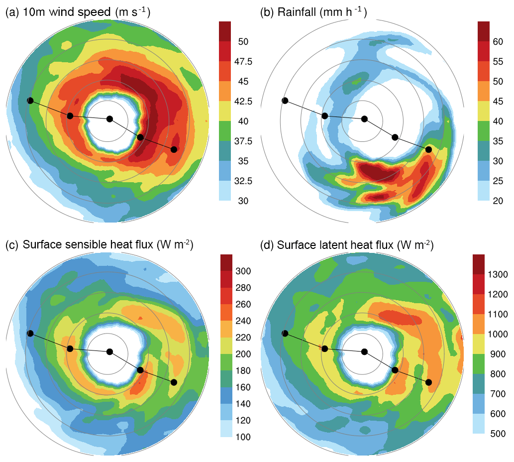
Figure 5Horizontal distributions for (a) wind speed (m s−1) at 10 m height, (b) total rainfall (mm h−1), (c) surface sensible heat flux (W m−2), and (d) surface latent heat flux (W m−2) at forecast hour 71 h (valid at 22:00 UTC on 7 November) for the experiment F0 with 3 km resolution. All fields are taken from the transformed subset on cylindrical grids; see text for detail. At 71 h, the simulated typhoon centered at the nearest location to the best-track location at 18:00 UTC on 7 November 2013. Range rings are shown at radii of 20, 40, 60, 80, and 100 km. Black dot at the plane center denotes the simulated typhoon center at 71 h, whereas the two dots to the upper left and lower right of this central dot are the corresponding locations of the typhoon center in the next and previous 2 h. Solid lines connecting these dots denote the simulated typhoon track within the 5 h.
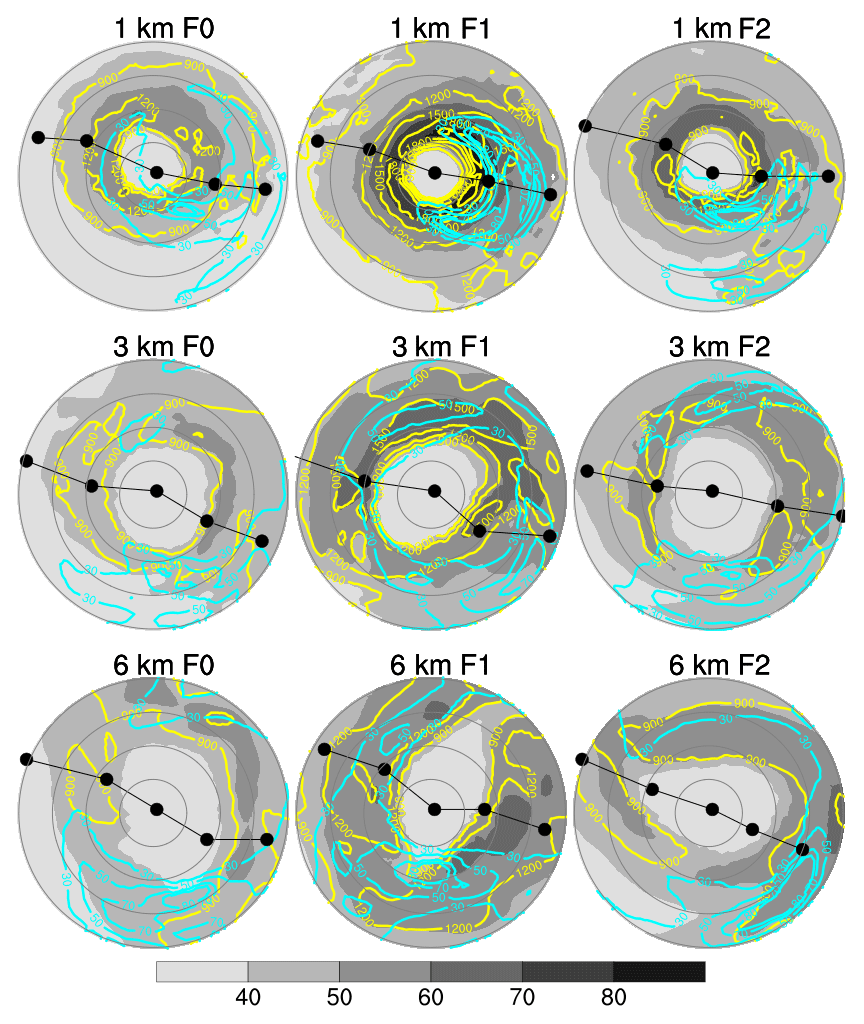
Figure 6Horizontal distributions for wind speed at 10 m height (shaded; m s−1), surface latent heat flux (yellow contours; W m−2), and total rainfall (cyan contours; mm h−1) at 71 h for all experiments. In all the experiments, the center location of the simulated typhoon at 71 h is at the nearest or the second nearest location to the best-track location at 18:00 UTC on 7 November 2013. The distributions for experiment F0 of 3 km resolution are the same as in Fig. 5 but slightly zoom in on a circle of radius 80 km; range rings are shown at radii of 20, 40, 60, and 80 km. Other symbols are shown as in Fig. 5.
We have examined these surface fields over the period from 12:00 UTC on 7 November to 00:00 UTC on 8 November and found similar features to those in Fig. 6, indicating that this period can be seen as the mature stage of the simulated typhoon. Overall, the horizontal distributions of the wind speed at 10 m height and total rainfall reveal a region of higher wind speed on the right (northern) side of the track and a region of intense rainfall to the left side of the rear side of the track. This result agrees with the study of Shimada et al. (2018) for Typhoon Haiyan. Based on the radar reflectivity measured several hours before the first landfall of Haiyan, they found that the region of the larger maximum wind speed was located on the right side of the track, and the region of stronger retrieved rainfall was located on the downshear-left side. During their analysis period (approximately 2.5 h immediately before Haiyan's first landfall), the 850–200 hPa vertical wind shear was north-northeasterly at about 4 m s−1. Therefore, the downshear-left side is approximately the left-rear side of the track. They found a slight southward vertical tilt (approximately 1 km from 1 to 7 km altitude) of the center of Haiyan, almost the same as the direction of the vertical tilt. We also found similar vertical wind shear of approximately 5 m s−1 at a northeasterly direction, as well as a small vertical tilt (about 1 grid box) of the storm center, during the 12 h period starting at 12:00 UTC on 7 November 2013 (data not shown). Accordingly, our simulations are in reasonable agreement with observations of Haiyan studied by Shimada et al. (2018).
The next step is to examine the azimuthal averages of the radius distribution for surface fields as well as the vertical structure of the simulated typhoon. For the radius distributions shown in Figs. 7, 8, 10, and 11, the track lines over a 3 h window (the two segments centered at that particular hour, as shown in Fig. 5) were used to identify the semicircles on both sides. Because a small deflection of the track tendency is generally found in the 3 h window, the areas of the right (northern) and left (southern) semicircles are not necessarily the same.
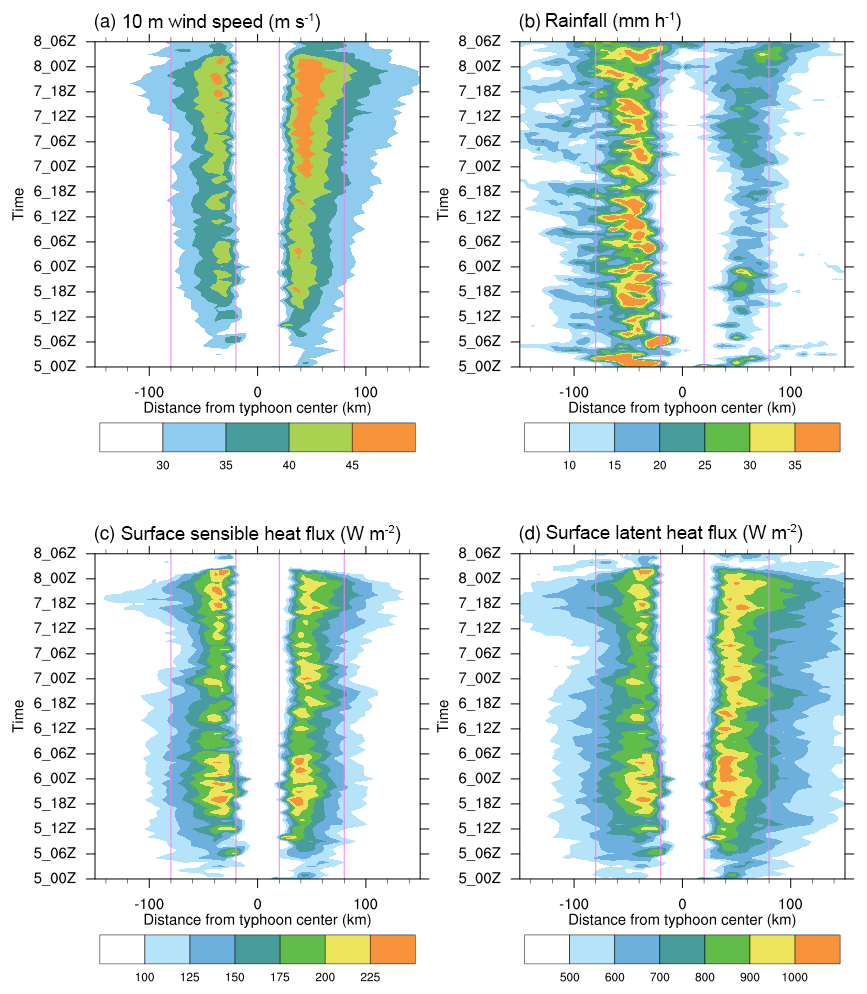
Figure 7Radius–time cross sections of (a) 10 m wind speed (m s−1), (b) rainfall (mm h−1), (c) surface sensible heat flux (W m−2), and (d) surface latent heat flux (W m−2) for the control experiment (3kmF0). The positive and negative distances from the typhoon center represent the azimuthal averages of the right (northern) and left (southern) semicircles, respectively, along the typhoon track. For each hourly output, the corresponding track in 3 h centered at that particular hour is used to identify the semicircles on both sides.
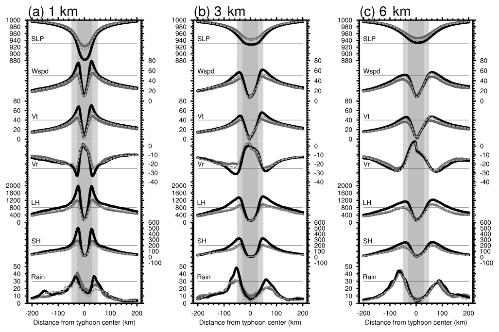
Figure 8The radial variations of surface fields for experiments 1 km (a), 3 km (b), and 6 km (c). The surface fields shown are (from top to bottom) sea level pressure (SLP; hPa), wind speed and tangential and radial winds at 10 m (Wspd, Vt, and Vr; m s−1), surface latent and sensible heat fluxes (LH and SH; W m−2), and total rainfall (Rain; mm h−1). Positive values of Vr indicate inflow. Gray, black, and gray-dashed curves represent flux options F0, F1, and F2, respectively. Horizontal gray lines are selected reference lines for each field. All fields are time averaged between 18:00 UTC on 7 November 2013 and 00:00 UTC on 8 November 2013. Positive and negative distances represent the right (northern) and left (southern) semicircles as in Fig. 7. Vertical light-gray and gray shaded bars denote the radial sectors bounded by radii of 50 and 30 km, respectively.
Figure 7 provides Hovmöller diagrams of the 10 m winds, total rainfall rate, and surface enthalpy (latent and sensible heat) fluxes for 3kmF0. Most noteworthy is the asymmetric structure found in the wind and rainfall fields. The stronger winds over the right (northern) side occurred in association with a larger rainfall rate over the left (southern) side of the typhoon center throughout the integration period. The asymmetric structure can also be found in the surface latent heat flux, whereas it is less evident in the surface sensible heat flux. Similar asymmetric patterns are found in all other simulations (data not shown). Figure 8 illustrates the composite of radial distributions of the selected surface fields for the mature stage, namely between 18:00 UTC on 7 November 2013 and 00:00 UTC on 8 November 2013, for the sensitivity experiments F0, F1, and F2. The patterns of F2 experiments are generally somewhat in between those of F0 and F1, with their wind field (enthalpy flux) patterns following those of F1 (F0) more closely. This is expected because F1 and F2 use an identical momentum transfer coefficient and F0 and F2 possess a similar behavior to the enthalpy transfer coefficients in terms of their magnitudes and wind-dependent variations.
We begin with the composite of 3 km resolution (Fig. 8b). During the mature stage, the radial patterns of mean sea level pressure (SLP) and 10 m winds reveal the typical structure of a tropical cyclone. The difference between the radii of maximum 10 m winds (RMWs) of 3kmF0 and 3kmF1 is insignificant. The tangential wind components dominate the 10 m wind fields. In both experiments, the radii of the maximum radial wind component are slightly larger than those of their respective tangential winds. In the context of azimuthal averages, the radial distributions of surface enthalpy fluxes are fundamentally constrained by the 10 m wind speed intensity. The aforementioned asymmetric pattern is again evident in the rainfall distribution and even in the wind fields. The 3kmF1 experiment yields a deeper storm central pressure and stronger wind speeds and enthalpy fluxes than the 3kmF0 experiment does. The 3kmF2 experiment produces similar patterns to the 3kmF0 experiment. The majority of these increments occur around the eyewall (in terms of the maximum winds). Increasing the grid spacing to 6 km yields a composite radial structure highly similar to the 3 km group, thus indicating the relationship among these near-surface fields (Fig. 8c). The major difference between the groups (6 and 3 km) is the size of the inner core with respect to the eyewall radius (measured in RMWs) and the sharpness of peaks in the near-surface fields. This is consistent with the aforementioned horizontal distributions of these surface fields shown in Fig. 6. As grid spacing decreases, RMWs decrease and the peak sharpness in winds and enthalpy fluxes increase. A much more marked decrease in RMWs and increase in peak sharpness are found in the 1 km resolution group than in the other groups (Fig. 8a). The SLPs, wind fields, and enthalpy fluxes in the 1 km group have narrow but sharp peaks, along with larger peak values compared with the other resolution groups. The asymmetric pattern of the wind fields is less evident but still can be seen. The 1kmF1 experiment yields a much stronger storm than the 1kmF0 experiment. The asymmetry of the rainfall pattern, however, decreases by using F1. At this point, whether the reduction of grid spacing or the use of more realistic flux formulas leads to a more symmetric (and thus more intense) tropical cyclone remains unclear.
In brief, both the increased resolution and more reasonable flux formulas enhance storm strength. Storm size (in terms of RMWs) is apparently sensitive to the changes in grid spacing but less sensitive to the choice of flux options. A reduction of storm size with smaller grid spacing has been noted by numerous studies (e.g., Davis et al., 2008; Fierro et al., 2009; Gentry and Lackmann, 2010; Kanada and Wada, 2016). As the strength of a storm increases, the eyewall contracts, indicating a higher efficiency of storm intensification with smaller grid spacing. In our work, the effect of different flux formulas on Typhoon Haiyan simulation is revealed by the changes in storm central pressure and the intensity of maximum winds and enthalpy fluxes around the eyewall. This implies that the underlying mechanisms (i.e., surface flux exchange processes) of various flux options account for storm intensity, whereas the reduction of grid spacing leads to more intense storm structures providing more conducive conditions for enhancing a positive flux effect.
Figure 9 shows the statistics for data points collected within a circle of radius 100 km during a sampling period of 7 h. From the percentages of binned wind speeds, the major pattern of the differences in flux options is revealed by a rightward shift of the curves in the order of F0, F2, and F1. For each resolution group, a reduction of the higher percentages of moderate to high wind speeds and the emergence of higher wind speeds are observed by comparing F2/F1 with F0. This feature is more evident in the distributions of 1 and 3 km resolution groups, in particular for the pattern shift of F1. This is to say that experiments with F1 can produce extremely high wind speeds (exceeds approximately 55 m s−1) as the resolution increases to 3 km as well as 1 km. For the 6 km resolution, less grid points (<5 %) with a wind speed of approximately 55 m s−1 are found even with flux option F1. This can also explain the comparable maximum wind speeds found in the F1 experiments with 3 and 6 km resolution (see Fig. 4c). The comparable storm intensities, in terms of minimum central pressure, found in 3 and 6 km resolutions (see Fig. 4b) are indeed in association with different near-surface wind speed distribution (also see Fig. 6). In 3 km as well as 1 km resolution, more extended and organized areas of extremely high wind speeds are found, whereas for 6 km resolution, broader areas of high wind speeds with a small amount of extremely high wind speed patches are found. The previous analyses indicate that the typhoon intensity is mainly controlled by the model resolution. The near-surface wind speed is an influential factor for the calculation of bulk transfer coefficients. Considering the low frequency of occurrences for extremely high wind speeds, the positive effect of the more reasonable surface option (F1) cannot be enhanced efficiently with a relatively large grid spacing of 6 km.
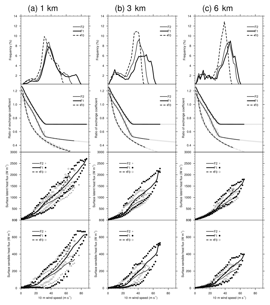
Figure 9The top panels are the percentage of samples in 2 m s−1 bins for wind speeds. These wind speed samples were collected inside a circle of radius 100 km with respect to the typhoon center at each output hour during a sampling period from 18:00 UTC on 7 November 2013 to 00:00 UTC on 8 November 2013. Over this sampling period of 7 h, only points over ocean are collected. The percentages were the number of data points in each wind speed bin divided by the total count during the sampling period. The upper middle, lower middle, and bottom panels show the binned averages and data ranges for the ratio of CK∕CD at 10 m height, latent heat flux, and sensible heat flux, respectively, in each 2 m s−1 wind speed bin. Here the values of CQ at 10 m height are used as CK. The binned averages are the mean values for the corresponding variable as collected in bins depending on the collocated wind speed and are displayed as solid or dashed curves. Within each wind speed bin, the respective data range for each variable is bounded by the minimum and maximum values from all binned samples during the period of 7 h. The data ranges are denoted as vertical bars (CK∕CD) and symbols (fluxes). Gray curves in the panels of CK∕CD are the same as in Fig. 2d, superimposed for reference.
Altogether, the wind speed statistics presented here suggest that more detailed structures over the full wind speed spectrum can only be resolved as the model resolution increases to up to 3 km or higher. This is consistent with the findings of Davis et al. (2008) and Gentry and Lackmann (2010) that a resolution of approximately 3 km or higher is required for significant improvement of intensity simulation of intense hurricanes (Hurricane Katrina in their case). With a lower resolution, 6 km in our case, we speculate that the momentum energy is diluted over the nearby grid points such that limited magnitude (higher but not extreme) of wind speeds would become evenly distributed over a broader area. This idea is specifically inspired by the studies of Bryan et al. (2003) and Miyamoto et al. (2013). We further discuss the energy distribution of these simulations in the next section.
The behaviors of CK∕CD show that the patterns almost strictly follow their respective curves as predicted by the calculation of the neutral condition using the pseudo-wind data (see Fig. 2d). The spread of data, as represented by the range, is rather small and is approximately 10 %–12 % of the magnitude of their respective binned averages. However, the resulting latent heat and sensible heat fluxes present a much larger spread of data on the wind speed bins. For lower wind speeds (and thus smaller mean values of fluxes), the range of data is approximately 90 % (150 %) of the magnitude of the binned mean. For high to extremely high wind speeds (and thus large mean values of fluxes), the range of data comes close to or less than 50 % (90 %) of the magnitude of the binned mean. A further inspection of the data reveals that the spread in binned data arises from the discrepancy in stability conditions near the ocean surface. This is expected as seen in Eqs. (A2) and (A3). For moderate to high wind speeds, given a value of latent heat or sensible heat flux, the corresponding wind speed ranges are considerably large. Therefore, the structure of near-surface moist-air enthalpy is also important for typhoon development. Furthermore, F1 can produce the largest latent and sensible heat fluxes between the three flux options, and the magnitude of the interoption differences increases as the resolution increases. This is obviously because of the larger percentage of extremely high wind speeds that F1 can achieve. Although the extremely high wind speeds comprise a small percentage of the eyewall circulation of a mature cyclone, they have a crucial role in enhancing surface fluxes that supply enthalpy to the eyewall.
As the resolution increases, the vertical distribution of tangential winds reveals a significant increase in the vertical extent of stronger wind speed, a reduction of the outward slope of the maximum wind axis, and thus a contraction of the eyewall (Fig. 10). With the change from F0 to F1, tangential wind speeds increase, with an outward and upward expansion of the region of stronger wind speed. No apparent changes are noted in the vertical slope and radius of the eyewall owing to the change in flux options. Both the composite inflow and outflow weaken as the resolution increases but enhance as the flux option changes from F0 to F1. Here, the maximum value of inflow (outflow) is 28.3 (−38.8) m s−1 in 1kmF0 but it is 33.6 (−44.5) m s−1 in 1kmF1. Moreover, the maximum cores of tangential winds descend and the depth of inflow decreases as the resolution increases. Overall, the patterns of F2 are somewhat between those of F0 and F1. In addition, we can see that the upper-level radial inflows are evident in the 1 km resolution group. The upper-level radial inflows are apparently weaker in the 3 km resolution group and are hardly found in the 6 km resolution group. The upper-level radial inflow above the upper outflow layer is related to the development of upper-level warming in the eye; this is addressed in Fig. 12.
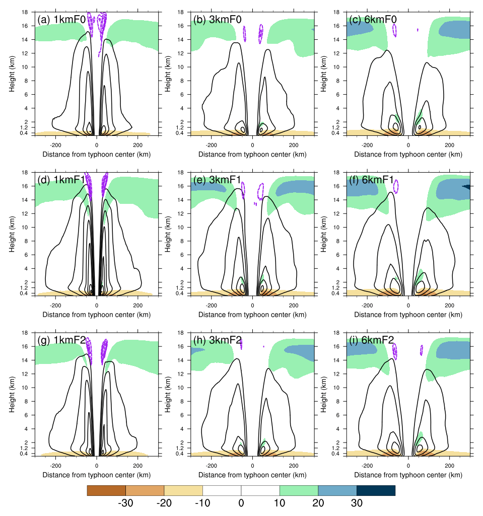
Figure 10Radius–height cross sections of tangential wind (contours; m s−1) superposed on radial wind (color shaded; m s−1) for experiments (a) 1kmF0, (b) 3kmF0, (c) 6kmF0, (d) 1kmF1, (e) 3kmF1, (f) 6kmF1, (g) 1kmF2, (h) 3kmF2, and (i) 6kmF2. The tangential winds are contoured every 10 m s−1 starting from 30 m s−1. Positive values of radial wind indicate inflow. The upper-level radial inflows (purple dashed contours; m s−1) are also superimposed and are contoured every 0.5 m s−1 starting from −0.5 m s−1. All fields are time averaged between 18:00 UTC on 7 November 2013 and 00:00 UTC on 8 November 2013. Positive and negative distances represent the right (northern) and left (southern) semicircles as in Fig. 7.
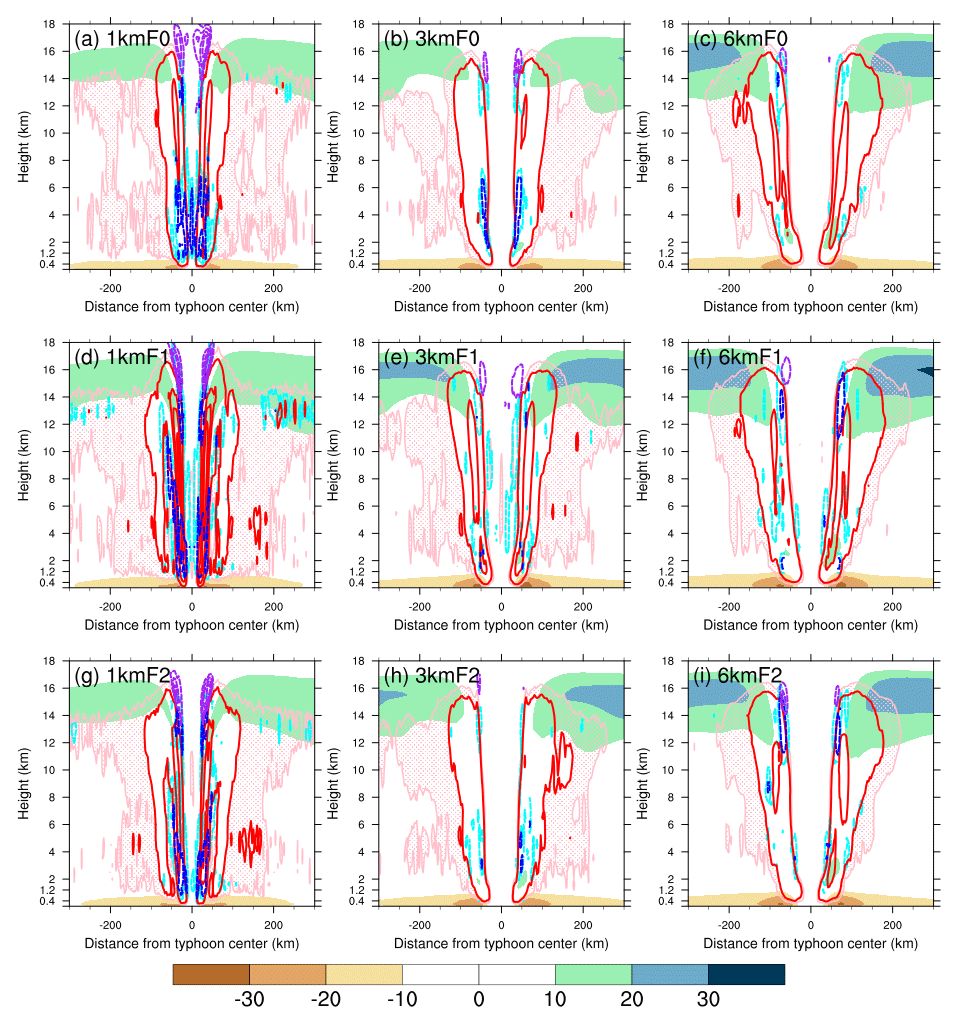
Figure 11The same as Fig. 10 but for vertical velocity (contours; m s−1) and radial wind (color shaded; m s−1). Positive (upward) and negative (downward) velocities are indicated by red and blue contours, respectively, and are plotted every 1 m s−1 starting from wind speeds of 0.5 m s−1. In addition, pink hatched areas denote an upward velocity of 0.3–0.5 m s−1; cyan contours denote a downward velocity of −0.3 m s−1.

Figure 12Time–height cross sections of upper-level radial inflow (contours; m s−1) superposed on the temperature anomaly (color shaded; K) for experiments (a) 1kmF0, (b) 3kmF0, (c) 6kmF0, (d) 1kmF1, (e) 3kmF1, (f) 6kmF1, (g) 1kmF2, (h) 3kmF2, and (i) 6kmF2. The upper-level radial inflows are contoured every 0.5 m s−1 starting from −0.5 m s−1. The temperature anomaly is defined with respect to a composite of domain-averaged temperature profiles at the model initial time of the sensitivity experiments (00:00 UTC on 5 November 2013); the composite of domain-averaged temperature profiles is derived as the mean of eight domain-averaged temperature profiles obtained from all the experiments. The time–height cross section of the temperature anomaly is the area-averaged temperature profile inside a ring of radius 21 km with respect to the typhoon center at each output hour minus the composite of domain-averaged temperature profiles. The upper-level radial inflows are the area-averaged radial winds inside a ring of radius 200 km with respect to the typhoon center at each output hour; only the radial winds above 9 km height are used for calculation.
The contraction of the eyewall with reduction of grid spacing is also revealed by a more upright eyewall updraft (Fig. 11). We start with the major eyewall updrafts and downdrafts as denoted by red and blue contours, respectively, in Fig. 11. The reduction of grid spacing also results in stronger updrafts and downdrafts, where the enhanced eyewall downdrafts may be a cause of the decrease in the depth of inflow. The convections outside of the eyewall (weaker upward velocity denoted by the pink hatched area) are apparent in the 1 km resolution group. For this resolution group, the outside convection in F1 is stronger than that in F0. The outside convection is a result of the azimuthally averaged upward velocity of the outer rainband. In the 3 km resolution group, the outside convections are weaker but still apparently shown. No outside convection can be clearly distinguished from the eyewall in the 6 km resolution group. As the resolution decreases, the model may not be able to resolve intense updraft cores in the eyewall as well as the outer rainband near the eyewall. The larger grid spacing can only resolve a broader area of weaker updraft instead. We further discuss this in the next section. Stronger inflow and outflow as well as broader eyewall updraft are found at the 6 km resolution, suggesting that secondary circulation is stronger at lower resolutions, similar to the finding of Fierro et al. (2009). We further examined the horizontal flow patterns near the altitudes of the upper outflow layer, both on model native grids and cylindrical grids, and confirmed that the upper-level flow patterns in the 6 km resolution group are more radially outward than the rotational component. As the resolution increases, the upper-level flow pattern becomes more rotational, and the radially outward component is suppressed. Because of such discrepancy in the upper-level flow pattern, the azimuthally averaged upper outflows (upper-level radial winds) in the 6 km resolution group are the strongest between the resolution groups.
The time evolution of the core temperature is represented by the temperature anomaly with respect to a reference mean temperature (Fig. 12). Here we term the positive temperature anomaly as warming. The distinct difference found among the resolution groups is the development of the upper-level warming layer within the eye. For the 1 km resolution group, the apparent upper-level warming layer appears above approximately 10 km within a deep warming column in the eye. The upper-level warming layers occur earlier in the experiments F1 and F2 (Fig. 12a, d, g). The warming layer in experiment 1kmF1 is the most intense among all the others. The timings of the upper-layer warming are associated with their respective upper-level radial inflows. The upper-level warming layer has long been recognized by observational studies (e.g., Hawkins and Imbembo, 1976) and numerical simulations (e.g., Zhang and Chen, 2012; Chen and Zhang, 2013; Wang and Wang, 2014). In recent years, the formation of the upper-level warming layer has been related to the rapid intensification of tropical cyclones (e.g., Zhang and Chen, 2012; Chen and Zhang, 2013; Wang and Wang, 2014). This upper-level warming layer, under hydrostatic balance and considering the enhanced effect due to the upper-level dryer and thinner conditions of air, can produce a much greater effect on the surface pressure falls than the lower-level warming (e.g., Zhang and Chen, 2012). Regarding the formation as well as the maintenance of the upper-level warming layer, Zhang and Chen (2012) emphasized the contribution from the high-potential-temperature air detrained from the lower stratosphere, whereas Chen and Zhang (2013) introduced the contribution from the air detrained from the convective bursts (anomalous intense updrafts) in the eyewall. Both studies revealed the importance of the upper-level radial inflow in the warm air detrainment onto the eye region. Wang and Wang (2014) reported that, in an environment with decreasing vertical wind shear, air detrained from the lower stratosphere as well as from the convective bursts could result from the development of convective bursts within the inner-core region.
From experiment F0 to F1, the upper-level warming layer enhances significantly (Fig. 12 a, d). Although both F0 and F1 with 1 km resolution can produce extremely intense updraft cores, the experiment F1 provides a larger energy source (through surface enthalpy fluxes) to the simulated typhoon than experiment F0 does. Therefore, the significantly enhanced upper-level warming layer found in the experiment 1kmF1 could result from the warm detrainment from the intense updrafts (may be seen as convective burst) in the eyewall. The pattern of the experiment F2 is again somewhat between those of F0 and F1. A similar development of the upper-level warming layer can also be found in the 3 km resolution group, but apparently weaker than that in the 1 km group. However, the development of upper-level radial inflow appears to precede the main warming for nearly 24–36 h. This may be partly attributed to the weaker contraction of the eyewall in the 3 km resolution group. The weaker upper-level radial inflow is perhaps another reason for this inconsistency in the time evolution. The 6 km resolution group does not present comparable development of this upper-level warming layer as in the 3 km group, again indicating that a resolution of 6 km is inadequate to resolve the details of structure and development of a strong typhoon like Haiyan (2013).
When the resolution increases, a more intense convection core can be resolved, leading to a rapid pressure decrease near the typhoon and a pressure gradient increase in the area. This change in the pressure field is presumably due to the enhanced diabatic heating near the typhoon eyewall. The larger pressure gradient force would reduce the RMW according to the gradient wind balance equation. The reduced RMW would then accompany an area of diabatic heating closer to the typhoon center. This contraction of the eyewall keeps decreasing the central pressure of the typhoon, yielding positive feedback for typhoon development. The enhancement of these processes is mainly related to the model grid spacings. Near-surface wind speed affects the calculation of bulk transfer coefficients. The positive effect of the more reasonable surface option (F1) cannot be enhanced efficiently unless an extremely large wind speed is generated through the reduction of grid spacing.
Several studies have reported that the reduction of grid spacing yielded a deeper, stronger, and more upright and contracted eyewall (e.g., Fierro et al., 2009; Gentry and Lackmann, 2010; Kanada and Wada, 2016). We also demonstrated that the size of updraft cores in the eyewall shrank and the region of downdraft increases as the resolution is increased. Furthermore, both updraft and downdraft become more intense with the reduction of grid spacing. These features have also been recognized in many studies (e.g., Fierro et al., 2009; Gentry and Lackmann, 2010; Gopalakrishnan et al., 2011; Kanada et al., 2012). In addition, large vertical transport of heat and moisture can result in stronger storms given that the model resolution is sufficiently high (e.g., Gopalakrishnan et al., 2011; Kanada et al., 2012).
We used contoured frequency by altitude diagrams (CFADs; Yuter and Houze, 1995) to examine the variability of convective cores over the region shown in Fig. 3 (the blue box). The CFADs is a statistical method for summarizing the vertical distributions of meteorological fields. A CFAD is constructed by collecting frequency distributions of a particular variable at evenly spaced altitudes within an area, compiling them into a two-dimensional (data bin and altitude) dataset, and portraying the data on a single contour plot. The ordinate in the plot represents the altitude variation, and the abscissa represents the frequency bin. For each altitude on a CFAD, the frequencies should add up to 100 %. For a given CFAD, each point depicts the frequency of occurrence of the data in that bin at a specific altitude. Accordingly, the CFADs ignore horizontal variability and provide a bulk statistical measure for comparing the vertical structure of evolving fields of cumulonimbus clouds or any convective systems. Here, we take Fig. 13a as an example. On this CFAD, there are higher percentages (e.g., bounded by 20 % of data per decibel relative to Z per kilometer, or % dBZ−1 km−1) found in the higher reflectivity bins at lower altitudes and found in the lower reflectivity bins at higher altitudes. The former can indicate convective cells or precipitations, whereas the latter can indicate snow or stratiform precipitation. Therefore, considering a set of CFADs for an evolving cumulonimbus clouds, say from the initiation to the mature stage, the maximum percentage at each altitude would change from vertically oriented to negatively tilted toward lower reflectivity values. More detailed interpretations of the use of CFADs can be found in the work by Yuter and Houze (1995).
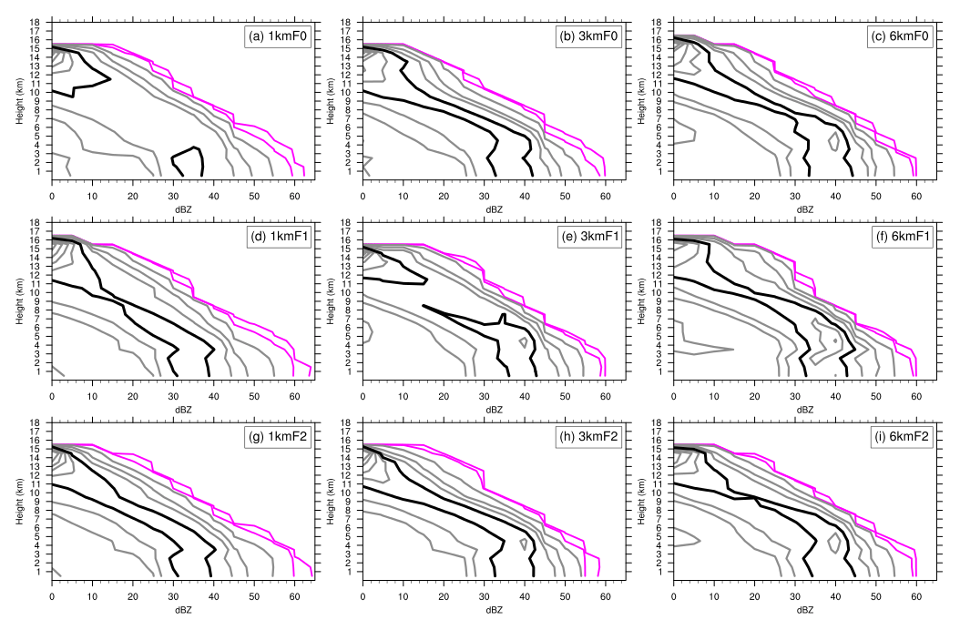
Figure 13The CFADs of simulated reflectivity for experiments (a) 1kmF0, (b) 3kmF0, (c) 6kmF0, (d) 1kmF1, (e) 3kmF1, (f) 6kmF1, (g) 1kmF2, (h) 3kmF2, and (i) 6kmF2. The sampling time for model output is taken as the simulated typhoon centered at its nearest location to the best-track location at 18:00 UTC on 7 November 2013 and for the following 2 h. The simulated reflectivity was taken from all grid points with updraft (positive vertical velocity) within the calculation domain for CFADs (see blue box in Fig. 3 for the corresponding area) in the model native grids. For reflectivity CFADs, the bin size is 5 dBZ and the plot is contoured at 0.01 %, 0.1 %, 1 %, 5 %, 10 %, 20 %, 30 %, 40 %, 50 %, and 60 % of data per decibel relative to Z per kilometer (% dBZ−1 km−1), with the 20 % dBZ−1 km−1 contour highlighted in black and the lowest two contours displayed in magenta.
CFADs of simulated reflectivity were conducted separately for updrafts and downdrafts (Figs. 13 and 14). In general, the CFADs of reflectivity derived from both updrafts and downdrafts present similar patterns. In these plots, a region bounded by a specific value, say 20 % dBZ−1 km−1, signifies that 80 % of the sampled data points are within this region. Taking the region bounded by the value of 20 % dBZ−1 km−1 as a reference, these plots reveal that approximately 80 % of the sampled data points in all the simulations present an increase in reflectivity with height above approximately 4 km; at heights lower than 4 km, reflectivity demonstrates little change. Similar patterns can be found in studies of CFADs of reflectivity for strong TCs in numerical simulations (Fierro et al., 2009) and for Florida cumulonimbi revealed by observational radar data (Yuter and Houze, 1995). Most noteworthy about our CFADs of reflectivity for both updrafts and downdrafts is the shrinking region bounded by a contour of 20 % dBZ−1 km−1 as the resolution increases. This indicates that at higher resolutions the range of reflectivity magnitudes presents a relatively broader distribution, which implies an increased occurrence of higher reflectivity. A descending of the core region of higher frequencies (as bounded by a contour of 20 % dBZ−1 km−1) is found in the CFADs of the downdraft compared with those of the updraft. According to the findings of Yuter and Houze (1995), this implies that the larger reflectivity at lower levels may be associated with the downdraft and thus can be interpreted as heavy precipitation, whereas higher reflectivity at approximately 4–5 km is mostly associated with updraft and, thus, may be seen as a convective cell. However, interpretations are different for reflectivity associated with updraft and downdraft here.

We further conducted CFADs of vertical motions to address this issue (Fig. 15). Most vertical velocities, carried by approximately 95 % of the data points as indicated by the region within the 1 % of data per meter per second per kilometer (% m−1 s km−1) contour, are apparently less than 5 m s−1 in all simulations. A similar pattern of CFADs of vertical velocity, revealing that most common values of vertical velocity are substantially low, can be found in numerical simulations for TCs (Fierro et al., 2009; Gentry and Lackmann, 2010; Wang and Wang 2014) and observational data for cumulonimbi (Yuter and Houze, 1995). Furthermore, the region of upward motion is larger than that of downward motion in general. A similar asymmetry of the distributions of upward and downward motion was evident in simulations in previous studies (Fierro et al., 2009; Gentry and Lackmann, 2010; Wang and Wang, 2014). In Fig. 15, the most significant differences in the CFADs of vertical velocity are revealed by the lower frequencies, namely the values of 1 % m−1 s km−1 and 0.1 % m−1 s km−1. As the resolution increases here, both upward and downward motion present an expansion of the distribution of the frequency of 1 % m−1 s km−1. However, the extents of the changes in upward and downward motions with resolution are different. In all simulations, the changes in the downward motion with an increased resolution are more significant than those in the upward motion. Therefore, the region (occurrence) of the downward motion increases as the resolution increases. The results also indicate the presence of less downdrafts in lower-resolution simulations (i.e., 3 and 6 km), and the degradation of available data points can result in large biases in the CFADs of reflectivity in association with the downdraft.
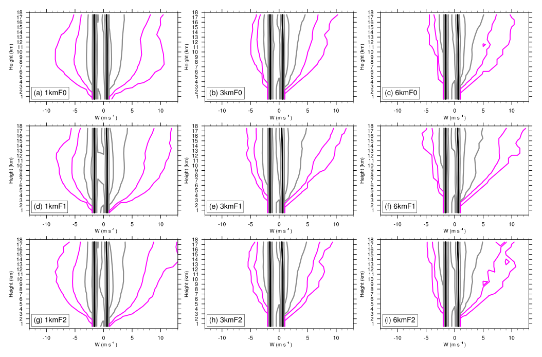
Figure 15The same as Fig. 14 but for CFADs of simulated vertical velocity. The velocity bin size is 1 m s−1 and the plot is contoured at 0.01 %, 0.1 %, 1 %, 5 %, 10 %, 20 %, 30 %, 40 %, 50 %, and 60 % of data per meter per second per kilometer (% m−1 s km−1), with the 20 % m−1 s km−1 contour highlighted in black and the lowest two contours displayed in magenta.
Finally, the 1 km simulations produce stronger updrafts and downdrafts than the 3 and 6 km simulations. Therefore, the higher reflectivity (indicated by the 0.1 % dBZ−1 km−1 contour) in 1 km simulations may be associated with much more intense updrafts compared with those in the 6 km simulations. This is consistent with the discrepancy between the secondary circulations of different resolutions in the previous section, where 6 km simulations presented relatively wider and weaker updrafts among the different resolutions. As previously mentioned, the CFADs of reflectivity in the 6 km simulations presented a relatively concentrated range of reflectivity magnitudes compared with the 1 km simulations, implying that the convective cells associated with the eyewalls may be broader in spatial scale. This is confirmed by an examination of horizontal distributions of the reflectivity of the 6 km resolution of simulations (data not shown). This can be interpreted as follows. As the resolution is insufficient to resolve the typical cumulonimbus size (∼10 km), a number of convective cells (e.g., cumulonimbus clouds) would be interpreted as a broader and perhaps stronger convective plume as discussed by Bryan et al. (2003) and Miyamoto et al. (2013). Bryan et al. (2003) attributed this broader convective plume to the diffusion due to subgrid-scale processes. In short, the intense reflectivity (convective) cores of the 1 km simulations are driven by extreme updrafts occurring within a rather small fraction of the CFAD's computational domain, whereas the 6 km simulations are driven by relatively weaker updrafts spread over a much broader spatial distribution.
In general, this resolution dependence of the spatial scale of updrafts may be attributed to the model effective resolution, namely the minimum scale resolved by the discretized model, as discussed by Skamarock (2004). By locating where the simulated energy slope drops below the expected slope, Skamarock (2004) found that the effective resolution of the WRF model at a grid spacing of 4–22 km is generally nearly 7-fold that of the model grid spacing (DX) and thus indicated that only information at scales greater than approximately 7 DX in energy spectra represents a physical solution for the WRF model. To examine the effective model resolution in our experiments, we adopted the algorithm of spectral computation introduced by Denis et al. (2002) for the calculation of kinetic energy (KE) spectra. Denis et al. (2002) introduced a two-dimensional discrete cosine transform to convert the limited domain of grid point atmospheric fields into spectral space. In this study, the spectral decompositions of velocities (u, v, and w) were first computed for each hourly model output and for each height level, and the KE spectra were then calculated from these velocity spectra. Finally, the KE spectra were averaged over selected periods and layers for Fig. 16. Because the results of different flux options are similar, only the experiments with F0 and F1 were plotted in Fig. 16. In all simulations, for the KE spectra derived from the horizontal velocity components, we find a model effective resolution of approximately 7 DX where the values of the KE spectra drop significantly, as indicated by Skamarock (2004). Although the vertical velocity spectra exhibit a flatter slope than the horizontal KE spectra, they also present apparent energy drops at wavelengths of approximately 6–7 DX. Our vertical velocity spectra show a pattern (i.e., the slopes) that is somewhat different from that of Bryan et al. (2003) with respect to the absence of peak values around the respective model effective resolutions. Bryan et al. (2003) conducted simulations with horizontal resolutions much higher than 1 km: 500, 250, and 125 m. With their extremely high resolutions, more intense convections could be resolved. They indicated that a model resolution of 1 km remains insufficient for explicitly resolving convective clouds. Here, we speculate that insufficient intense convection cores in our simulations may result in the absence of peak values around the respective model effective resolutions.

Figure 16Mean KE spectra for horizontal wind (a, b) and vertical velocity (c, d) for all simulations as computed over the boundary layer (a, c; between 1 and 2 km) and free troposphere (b, d; between about 3 and 8 km) for the mature stage. The mature stage is indicated by the average between 18:00 UTC on 7 November 2013 and 00:00 UTC on 8 November 2013. The gray lines correspond to the expected slopes for the large scale (−3 slope) and mesoscale to smaller scales ( slope) of the atmospheric kinetic energy spectrum. The wavelength and wavenumber are given on the lower and upper x axes, respectively. The purple triangles in each panel, from left to right, denote the locations of 7 DX for the simulations of resolutions 6, 3, and 1 km, respectively. The domain of the spectral decomposition is shown in Fig. 3.
Finally, the slope of the physical portion of the spectra (for the horizontal and vertical components, respectively) remains essentially unchanged as the model resolution is varied. In general, the higher the resolution, the further the downscale extent is, the smaller the scales represented are, and the smaller the model effective resolutions reached are. The aforementioned descriptions remain true for all flux options and averaging layers in our work. The key point is that the effective resolution is determined by grid spacing, not the flux options. We noted some subtle differences between the F0 and F1 experiments at smaller wavelengths at nearly 2 DX in the KE spectra but in only a few hours of the entire simulation period. In short, although the use of more reasonable flux formulas can increase simulated storm intensity to some extent, the positive effect of the flux formulas cannot be efficiently enhanced unless the grid spacing is appropriately reduced to yield intense and contracted eyewall structure.
This study investigated the effects of resolution and surface flux formulas on typhoon intensity and structure simulations through the case study of Super Typhoon Haiyan (2013). The effect could be separated between horizontal resolution and air–sea flux parameterization through the inner-core structure and spectral analyses. Specifically, we found significantly increased sensitivity of TC intensity simulations to surface flux parameterizations when model resolution approached the convective scale (∼1 km).
Three sets of surface flux formulas in the WRF model were tested using grid spacings of 1, 3, and 6 km. Increased resolution and more reasonable flux parameterization could both improve typhoon intensity simulation to a certain extent, but their effects on storm structures differed. A combination of decreasing momentum transfer coefficient and increasing enthalpy transfer coefficients tends to yield a stronger storm. The storm size (in terms of the radius of maximum winds) is apparently sensitive to the changes in grid spacing. The choice of flux formulas had little effect on storm size. Sufficiently high resolution was more conducive to the positive effect of flux formulas on simulated typhoon intensity.
Reducing the grid spacing to 1 km yielded a deeper, stronger, and more upright and contracted eyewall. Stronger inflow and outflow as well as relatively wider and weaker eyewall updraft were found in the lower resolutions, indicating a stronger secondary circulation. As strength increased, the eyewall contracted, indicating higher efficiency of storm intensification in smaller grid spacing. This contraction of eyewall is associated with an upper-level warming layer, which signifies an intense development of the simulated typhoon. The upper-level warming process can be attributed to the air detrained from the intense updraft cores in the eyewall, which can only be resolved by higher resolutions, such as 1 or 3 km.
The analysis of the CFADs revealed that the size of updraft cores in the eyewall shrinks and the region of downdraft increases, and both updraft and downdraft become more intense as the resolution increases. Therefore, the intense reflectivity (convective) cores of the higher-resolution simulations are driven by more intense updrafts within a rather small fraction of the spatial area, whereas lower-resolution simulations are driven by relatively weaker updrafts spread over a much broader spatial distribution. This resolution dependence of the spatial scale of updrafts is attributable to the model effective resolution based on the analysis of KE spectra. The effective resolution is determined by grid spacing, not the flux options. The analyses indicate that typhoon intensity is mainly controlled by the model resolution. Higher frequency of occurrences for extremely high wind speeds can be found in experiments with higher resolution. The near-surface wind speed is an influential factor for the calculation of bulk transfer coefficients. Although the use of more reasonable flux formulas can increase the simulated storm intensity to some extent, the positive effect of surface flux formulas cannot be efficiently enhanced unless the grid spacing is properly reduced to yield intense and contracted eyewall structure.
Although both updraft and downdraft cores within the eyewall can be partially resolved at 1 km grid spacing, model convergence does not emerge here (e.g., Bryan et al., 2003; Gentry and Lackmann, 2010; Miyamoto et al., 2013). The conducive effect for grid spacing well below 1 km to the contribution of flux parameterization needs to be further explored. Finally, the typhoon intensity in the experiment 1kmF1 is apparently overestimated. Green and Zhang (2013) suggested that the overestimation of their simulated TC intensity, compared with the observed best track, may be partially attributed to the neglect of ocean feedback in the model. This is also true in our case. Other components of the numerical model such as boundary layer mixing and the inclusion of wind wave coupling as well as ocean coupling are related to air–sea flux estimates, which is important for ocean feedback (e.g., Davis et al., 2008; Chen et al., 2007, 2010; Zhao et al., 2017). This is beyond the scope of this paper; however, further relevant research and additional simulation comparisons to other storms for generalizing our results are warranted.
The National Centers for Environmental Prediction Global Forecast System (GFS) operational global analysis dataset can be downloaded from the website https://www.ncdc.noaa.gov/data-access/model-data/model-datasets/global-forcast-system-gfs/ (last access: 20 July 2019; Environmental Modeling Center 2003, 2016). The RTG-SST dataset is available for download at ftp://polar.ncep.noaa.gov/pub/history/sst/ (last access: 20 July 2019; Gemmill et al., 2007). The WMO subset of the IBTrACS (IBTrACS-WMO, v03r09) can be accessed at ftp://eclipse.ncdc.noaa.gov/pub/ibtracs/v03r09/wmo/ (last access: 20 July 2019; Knapp et al., 2010). Appendix B provides the information of the observational estimates of surface flux.
(a) Fluxes in the atmospheric surface layer
In the surface layer, the vertical fluxes of horizontal momentum τ, sensible heat H, and latent heat LH near the surface are generally parameterized using bulk flux formulations:
where ρ is the air density; cp the specific heat capacity of air at constant pressure; Lv the latent heat of vaporization; u∗ the friction velocity, a velocity scale for the turbulent flow; θ∗ and q∗ the scaling parameters for potential temperature θ and specific humidity q, respectively; and CD, CH, and CD the dimensionless bulk transfer coefficients for momentum, sensible, and latent heat, respectively. The vertical differences in horizontal velocity, temperature, and specific humidity are enclosed in the parentheses in their respective bulk formulas, where the subscripts a and s denote the variable at a reference height and on the ground or water surface, respectively. Moreover, 10 m is frequently assumed as the reference height. The three bulk transfer coefficients should all correspond to the same reference height above the surface. Because the wind speed just on the ground surface is zero and the surface current over water may be set to zero for the sake of simplicity, the bulk formula for the vertical flux of the horizontal momentum can be reduced to ; thereafter, we omit the subscript a for brevity.
(b) Surface layer scheme in WRF
In WRF, the scaling parameters, bulk transfer coefficients, and all surface fluxes (momentum, sensible heat, and latent heat) are parameterized in a surface layer scheme. There are eight surface layer schemes available in the WRF-ARW, and seven of them are constructed based on the Monin–Obukhov similarity theory with somewhat different formulations, including those of the roughness lengths, bulk transfer coefficients, and the nondimensional stability functions defined for wind and potential temperature profiles. Among these available schemes, the surface layer scheme based on MM5 parameterization (Grell et al., 1994) has been widely used for a broad range of atmospheric research. In this study, we used the revised version of the MM5 surface layer scheme that has been implemented in the WRF model before version 3.2 (Jiménez et al., 2012). Considering that some details of the scheme can change over time, we compared the corresponding routines in WRF-ARW to the formulations in Jiménez et al. (2012) and found some discrepancies. During the time of writing this article, we referred to the WRF routines wherever there is a discrepancy found. Below, we briefly describe the most relevant features of the revised MM5 scheme for our work. Because our focus is on the TC intensity over the ocean, we only document the bulk transfer coefficients over the water surface.
(c) Flux parameterization used in this study
Based on the Monin–Obukhov flux–profile relationship, the scaling parameters u∗ and θ∗ are given as follows:
where κ is the von Karman constant; L is the Obukhov length; z is a specific height level; and z0 and zh are the roughness lengths for momentum and sensible heat, respectively. All roughness lengths are in meters. The Obukhov length L can be calculated from the relation
where g is the gravitational acceleration. The Monin–Obukhov stability functions for momentum (ψm) and heat (ψh) are calculated according to variant stability regimes defined in terms of the bulk Richardson number. The details of the stability functions can be found in Jiménez et al. (2012). The scaling parameter, as well as the stability function for moisture, is assumed to be the same as that for the sensible heat.
The bulk transfer coefficients for momentum and sensible heat are given as follows:
The bulk transfer coefficient for latent heat over water surface is given as follows:
where zq is the roughness length for latent heat. Jiménez et al. (2012) expressed the stability parameter as in their formulas of CH and CQ (see their Eqs. 21 and 22). In this version of the revised MM5 scheme, and are used for CH and CQ, respectively. Furthermore, the first term enclosed in the second bracket on the right side of the CQ formula is mainly valid for land surface as presented in Jiménez et al. (2012; see their Eq. 22). In our Eq. (A9), the corresponding term is expressed as for water surface according to the WRF routines.
According to the formulations of CD, CH, and CQ, the behaviors of these bulk transfer coefficients are strongly dependent on the momentum and scalar (heat and moisture) roughness lengths (see Eqs. A7, A8, and A9). The contribution of momentum roughness length z0 is perhaps more significant than the rest of two. On the right side of the CD formula, the three terms inside the bracket in the denominator are expressed in terms of z0. Here, we term the whole expression with brackets in the denominator in Eq. (A7) as a drag-dependent effect. A comparison of these formulas indicates that the expressions inside the first brackets on the right side of the CH and CQ formulas are both identical to the expression of the drag-dependent effect in Eq. (A7). In this context, CH and CQ shall vary with wind speed due to the drag-dependent effect even with an invariant scalar roughness length.
Table B1 provides brief information of the observational estimates shown in Fig. 2. For low-wind-speed conditions (wind speed roughly less than 5 m s−1), Vickers et al. (2013) indicated a decrease in CD with wind speed, in agreement with that observed in COARE 3.0 (Fairall et al., 2003; their Fig. 5), whereas Geernaert et al. (1987) and Large and Pond (1981) suggested a nearly constant (no trend) CD. For moderate-wind conditions (approximate range of 5–20 m s−1), Large and Pond (1981) and Vickers et al. (2013) indicated that the momentum transfer coefficient CD monotonically increases with wind speed (see Fig. 2a). An upward trend of CD has also been reported in Geernaert et al. (1987) and French et al. (2007), although the spread of their respective data is large. This is because shown in Fig. 2 are their data points rather than binned averages or fitted curves. Three sets of available estimates (Jarosz et al., 2007; Powell et al., 2003; Richter et al., 2016) revealed that the upward trend in CD would cease under high-wind conditions (approximate range of 25–55 m s−1), where a leveling-off or even a downward trend would occur instead. According to these observational estimates, the turning points of the wind-speed-dependent CD variations were varied and found within a range of 30 to 40 m s−1. Under the much stronger wind conditions (exceeding 55 m s−1), the behavior of CD again differs considerably from the relatively lower range of wind speeds. Bell et al. (2012) and Richter et al. (2016) suggested a rebound of CD values with wind speeds up to approximately 70 m s−1. However, there are also larger spreads of the CD values found.
There are fewer observational estimates of the heat and moisture transfer coefficient reported in literature, compared with the momentum transfer coefficient. Practically, the transfer coefficient for moist-air enthalpy surface flux (CK) was estimated in a number of studies (e.g., Zhang et al., 2008; Bell et al., 2012; Richter et al., 2016). A similar expression to Eqs. (A2) and (A3) can be derived for the moist-air-specific enthalpy flux, where the specific enthalpy is given as (Emanuel, 1995). Most studies suggested that the bulk transfer coefficients for scalar fields (i.e., sensible heat and moisture as well as enthalpy) are nearly independent of wind speed, with their respective mean values being 0.7 to (e.g., Geernaert, 1987; Smith, 1988; Drennan et al., 2007; Zhang et al., 2008; Bell et al., 2012; Richter et al., 2016). However, Fairall et al. (2003) reported a steady increase in CQ with wind speed based on the COARE dataset. Within the range of uncertainty, it is plausible to assume CQ=CK (e.g., Richter et al., 2016) or even (e.g., Emanuel, 1995; Zhang et al., 2008).
Table B1Summary of the previous studies for the observational estimates used in Fig. 2. The first column identifies the studies collected for the data extraction and the source (equation, figure, or table) in the corresponding literature. The second column gives the approximate range of the wind speed over which the bulk parameters were estimated; these are not the binned ranges in some of the literature. The third column describes the method of flux estimation and the observational data source (field experiments) used in these studies. ADCP: acoustic Doppler current profiler; CBLAST: Coupled Boundary Layer Air-Sea Transfer; GPS: Global Positioning System.
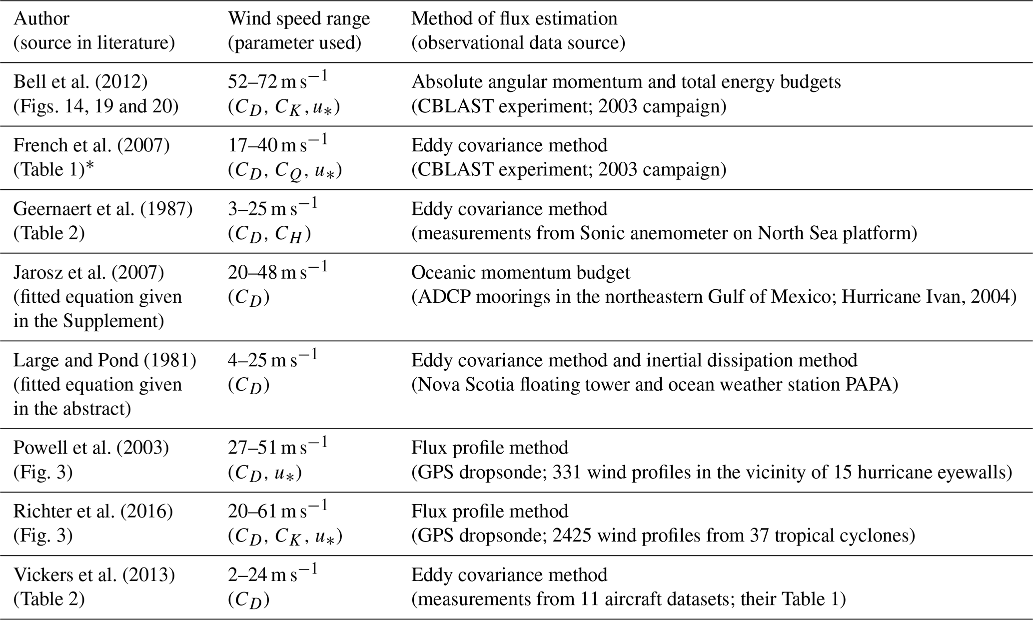
* The values of CQ were obtained from Table 1 of French et al. (2007), whereas the corresponding data analyses were reported by Drennan et al. (2007).
The supplement related to this article is available online at: https://doi.org/10.5194/nhess-19-1509-2019-supplement.
MTK designed the experiments and analyzed and prepared the manuscript with contributions from all co-authors. WMC, YFS, SCL, and EY performed the simulations and processed and analyzed the model output. TRW, YLT, and CYL joined the discussions of the study. All authors contributed to the preparation of this paper.
The authors declare that they have no conflict of interest.
We thank the two anonymous reviewers for their constructive comments and suggestions. An earlier version of the manuscript was edited by Wallace Academic Editing.
This research has been supported by the Ministry of Science and Technology, Taiwan (grant nos. 105-2111-M-001-003 and 106-2111-M-001-009).
This paper was edited by Ricardo Trigo and reviewed by two anonymous referees.
Atkinson, G. D. and Holliday, C. R.: Tropical cyclone minimum sea level pressure/maximum sustained wind relationship for the western North Pacific, Mon. Weather Rev., 105, 421–427, 1977.
Bao, J.-W., Gopalakrishnan, S. G., Michelson, S. A., Marks, F. D., and Montgomery, M. T.: Impact of physics representations in the HWRFX model on simulated hurricane structure and wind–pressure relationships, Mon. Weather Rev., 140, 3278–3299, https://doi.org/10.1175/MWR-D-11-00332.1, 2012.
Bell, M. M., Montgomery, M. T., and Emanuel, K. A.: Air–sea enthalpy and momentum exchange at major hurricane wind speeds observed during CBLAST, J. Atmos. Sci., 69, 3197–3222, https://doi.org/10.1175/JAS-D-11-0276.1, 2012.
Bender, M. A., Knutson, T. R., Tuleya, R. E., Sirutis, J. J., Vecchi, G. A., Garner, S. T., and Held, I. M.: Modeled impact of anthropogenic warming on the frequency of intense Atlantic hurricanes, Science, 327, 454–458, https://doi.org/10.1126/science.1180568, 2010.
Braun, S. A. and Tao, W.-K.: Sensitivity of high-resolution simulations of Hurricane Bob (1991) to planetary boundary layer parameterizations, Mon. Weather Rev., 128, 3941–3961, 2000.
Brutsaert, W.: A theory for local evaporation (or heat transfer) from rough and smooth surfaces at ground level, Water Resour. Res., 11, 543–550, 1975a.
Brutsaert, W.: The Roughness Length for Water Vapor, Sensible Heat, and other Scalars, J. Atmos. Sci., 32, 2028–2031, 1975b.
Brutsaert, W.: Heat and mass transfer to and from surfaces with dense vegetation or similar permeable roughness, Bound.-Layer Meteor., 16, 365–388, 1979.
Bryan, G. H., Wyngaard, J. C., and Fritsch, J. M.: Resolution requirements for the simulation of deep moist convection, Mon. Weather Rev., 131, 2394–2416, 2003.
Charnock, H.: Wind stress on a water surface, Q. J. Roy. Meteor. Soc., 81, 639–640, 1955.
Chen, H. and Zhang, D.-L.: On the rapid intensification of Hurricane Wilma (2005). Part II: Convective bursts and the upper-level warm core, J. Atmos. Sci., 70, 146–162, https://doi.org/10.1175/JAS-D-12-062.1, 2013.
Chen, S., Campbell, T. J., Jin, H., Gabersek, S., Hodur, R. M., and Martin, P.: Effect of Two-Way Air–Sea Coupling in High and Low Wind Speed Regimes, Mon. Weather Rev., 130, 3579–3602, https://doi.org/10.1175/2009MWR3119.1, 2010.
Chen, S. S., Price, J. F., Zhao, W., Donelan, M. A., and Walsh, E. J.: The CBLAST-Hurricane program and the next-generation fully coupled atmosphere-wave-ocean models for hurricane research and prediction, B. Am. Meteorol. Soc., 88, 311–317, https://doi.org/10.1175/BAMS-88-3-311, 2007.
Coronel, R., Sawada, M., and Iwasaki, T.: Impacts of Surface Drag Coefficient and Planetary Boundary Layer Schemes on the Structure and Energetics of Typhoon Megi (2010) during Intensification, J. Meteor. Soc. Japan. Ser. II, 94, 55–73, https://doi.org/10.2151/jmsj.2016-004, 2016.
Davis C., Wang, W., Chen, S. S., Chen, Y., Corbosiero, K., DeMaria, M., Dudhia, J., Holland, G., Klemp, J., Michalakes, J., Reeves, H., Rotunno, R., Snyder, C., and Xiao, Q.: Prediction of landfalling hurricanes with the advanced hurricane WRF model, Mon. Weather Rev., 136, 1990–2005, https://doi.org/10.1175/2007MWR2085.1, 2008.
Denis, B., Cote, J., and Laprise, R.: Spectral decomposition of two dimensional atmospheric fields on limited-area domains using the discrete cosine transform (DCT), Mon. Weather Rev., 130, 1812–1829, 2002.
Donelan, M. A., Haus, B. K., Reul, N., Plant, W. J., Stiassnie, M., Graber, H. C., Brown, O. B., and Saltzman, E. S.: On the limiting aerodynamic roughness of the ocean in very strong winds, Geophys. Res. Lett., 31, L18306, https://doi.org/10.1029/2004GL019460, 2004.
Drennan, W. M., Zhang, J. A., French, J. R., McCormick, C., and Black, P. G.: Turbulent fluxes in the hurricane boundary layer. Part II: Latent heat flux, J. Atmos. Sci., 64, 1103–1115, 2007.
Emanuel, K. A.: An air–sea interaction theory for tropical cyclones. Part I: Steady-state maintenance, J. Atmos. Sci., 43, 585–604, 1986.
Emanuel, K. A.: Sensitivity of tropical cyclones to surface exchange coefficients and a revised steady-state model incorporating eye dynamics, J. Atmos. Sci., 52, 3969–3976, 1995.
Environmental Modeling Center: The GFS atmospheric model, NCEP Office Note 442, 14 pp., available at: http://www.emc.ncep.noaa.gov/officenotes/newernotes/on442.pdf (last access: 24 July 2019), data available at: https://www.ncdc.noaa.gov/data-access/model-data/model-datasets/global-forcast-system-gfs/ (last access: 20 July 2019), 2003.
Environmental Modeling Center: The Global Forecast System (GFS) – Global Spectral Model (GSM), available at: https://www.emc.ncep.noaa.gov/GFS/doc.php (last access: 24 July 2019), data available at: https://www.ncdc.noaa.gov/data-access/model-data/model-datasets/global-forcast-system-gfs/ (last access: 20 July 2019), 2016.
Fairall, C. W., Bradley, E. F., Hare, J. E., Grachev, A. A., and Edson, J. B.: Bulk parameterization of air–sea fluxes: Updates and verification for the COARE algorithm, J. Climate, 16, 571–591, 2003.
Fierro, A. O., Rogers, R. F., Marks, F. D., and Nolan, D. S.: The impact of horizontal grid spacing on the microphysical and kinematic structures of strong tropical cyclones simulated with the WRF-ARW model, Mon. Weather Rev., 137, 3717–3743, https://doi.org/10.1175/2009MWR2946.1, 2009.
French, J. R., Drennan, W. M., Zhang, J. A., and Black, P. G.: Turbulent fluxes in the hurricane boundary layer. Part I: Momentum flux, J. Atmos. Sci., 64, 1089–1102, https://doi.org/10.1175/JAS3887.1, 2007.
Geernaert, G. L., Larsen, S. E., and Hansen, F.: Measurements of wind stress, heat flux, and turbulence intensity during storm conditions over the North Sea, J. Geophys. Res., 92, 13127–13139, 1987.
Gemmill, W., Katz, B., and Li, X.: Daily real-time, global sea surface temperature – high-resolution analysis: RTG_SST_HR. NOAA/NCEP. NOAA/NWS/NCEP/MMAB Office Note Nr. 260, 39 pp., available at: https://polar.ncep.noaa.gov/mmab/papers/tn260/ (last access: 19 July 2019), data available at: ftp://polar.ncep.noaa.gov/pub/history/sst/ (last access: 20 July 2019), 2007.
Gentry, M. S. and Lackmann, G. M.: Sensitivity of simulated tropical cyclone structure and intensity to horizontal resolution, Mon. Weather Rev., 138, 688–704, https://doi.org/10.1175/2009MWR2976.1, 2010.
Gopalakrishnan, S. G., Marks Jr., F., Zhang, X., Bao, J.-W., Yeh, K.-S., and Atlas, R.: The experimental HWRF system: A study on the influence of horizontal resolution on the structure and intensity changes in tropical cyclones using an idealized framework, Mon. Weather Rev., 139, 1762–1784, do:10.1175/2010MWR3535.1, 2011.
Green, B. W. and Zhang, F.: Impacts of air–sea flux parameterizations on the intensity and structure of tropical cyclones, Mon. Weather Rev., 141, 2308–2324, https://doi.org/10.1175/MWR-D-12-00274.1, 2013.
Grell, G. A., Dudhia, J., and Stauffer, D. R.: A description of the fifth-generation Penn State/NCAR Mesoscale Model (MM5), NCAR Tech. Note NCAR TN-398-1-STR, 117 pp., 1994.
Hawkins, H. F. and Imbembo, S. M.: The structure of a small, intense hurricane—Inez 1966, Mon. Weather Rev., 104, 418–442, https://doi.org/10.1175/1520-0493(1976)104<0418:TSOASI>2.0.CO;2, 1976.
Hill, K. A. and Lackmann, G. M.: Analysis of Idealized Tropical Cyclone Simulations Using the Weather Research and Forecasting Model: Sensitivity to Turbulence Parameterization and Grid Spacing, Mon. Weather Rev., 137, 745–765, https://doi.org/10.1175/2008MWR2220.1, 2009.
Hong, S.-Y., Dudhia, J., and Chen, S.-H.: A revised approach to ice microphysical processes for the bulk parameterization of clouds and precipitation, Mon. Weather Rev., 132, 103–120, 2004.
Hong, S.-Y., Noh, Y., and Dudhia, J.: A new vertical diffusion package with an explicit treatment of entrainment processe, Mon. Weather Rev., 134, 2318–2341, https://doi.org/10.1175/MWR3199.1, 2006.
Iacono, M. J., Delamere, J. S., Mlawer, E. J., Shephard, M. W., Clough, S. A., and Collins, W. D.: Radiative forcing by long–lived greenhouse gases: Calculations with the AER radiative transfer models, J. Geophys. Res., 113, D13103, https://doi.org/10.1029/2008JD009944, 2008.
Jarosz, E., Mitchell, D. A., Wang, D. W., and Teague, W. J.: Bottom-up determination of air–sea momentum exchange under a major tropical cyclone, Science, 315, 1707–1709, https://doi.org/10.1126/science.1136466, 2007.
Jiménez, P. A., Dudhia, J., González-Rouco, J. F., Navarro, J., Montávez, J. P., and García-Bustamante, E.: A revised scheme for the WRF surface layer formulation, Mon. Weather Rev., 140, 898–918, https://doi.org/10.1175/MWR-D-11-00056.1, 2012.
Kain, J.: The Kain–Fritsch convective parameterization: An update, J. Appl. Meteor. Climatol., 43, 170–181, 2004.
Kain, J. S. and Fritsch, J. M.: A one–dimensional entraining/detraining plume model and its application in convective parameterization, J. Atmos. Sci., 47, 2784–2802, 1990.
Kanada, S. and Wada, A.: Sensitivity to horizontal resolution of the simulated intensifying rate and inner-core structure of Typhoon Ida, an extremely intense typhoon, J. Meteor. Soc. Japan, 94A, 181–190, https://doi.org/10.2151/jmsj.2015-037, 2016.
Kanada, S., Wada, A., Nakano, M., and Kato, T.: Effect of planetary boundary layer schemes on the development of intense tropical cyclones using a cloud-resolving model, J. Geophys. Res., 117, D03107, https://doi.org/10.1029/2011JD016582, 2012.
Knaff, J. A. and Zehr, R. M.: Reexamination of tropical cyclone wind–pressure relationships, Weather Forecast., 22, 71–88, https://doi.org/10.1175/WAF965.1, 2007.
Knapp, K. R., Kruk, M. C., Levinson, D. H., Diamond, H. J., and Neumann, C. J.: The International Best Track Archive for Climate Stewardship (IBTrACS): Unifying tropical cyclone best track data, B. Am. Meteorol. Soc., 91, 363–76, https://doi.org/10.1175/2009BAMS2755.1, (data available at: ftp://eclipse.ncdc.noaa.gov/pub/ibtracs/v03r09/wmo/ (last access: 20 July 2019), 2010.
Knapp, K. R., Knaff, J. A., Sampson, C. R., Riggio, G. M., and Schnapp, A. D.: A pressure-based analysis of the historical western North Pacific tropical cyclone intensity record, Mon. Weather Rev., 141, 2611–-2631, https://doi.org/10.1175/MWR-D-12-00323.1, 2013.
Koba, H., Osano, S., Hagiwara, T., Akashi, S., and Kikuchi, T.: Relationship between the CI-number and central pressure and maximum wind speed in typhoons, Geophy. Mag., 44, 15–25, 1991 (in English).
Kueh, M.-T.: Multiformity of the tropical cyclone wind–pressure relationship in the western North Pacific: Discrepancies among four best-track archives, Environ. Res. Lett., 7, 024015, https://doi.org/10.1088/1748-9326/7/2/024015, 2012.
Lander, M., Guard, C., and Camargo, S.: Super Typhoon Haiyan, in: State of the Climate in 2013, B. Am. Meteorol. Soc., 95, S112–S114, 2014.
Large, W. G. and Pond, S.: Open ocean momentum flux measurements in moderate to strong winds, J. Phys. Oceanogr., 11, 324–336, 1981.
Large, W. G. and Pond, S.: Sensible and latent heat flux measurements over the ocean, J. Phys. Oceanogr., 12, 464–482, 1982.
Li, F., Song, J., and Li, X.: A preliminary evaluation of the necessity of using a cumulus parameterization scheme in high-resolution simulations of Typhoon Haiyan (2013), Nat. Hazards, 92, 647–671, https://doi.org/10.1007/s11069-018-3218-y, 2018.
Lin, I.-I., Pun, I.-F., and Lien, C.-C.: “Category-6” super typhoon Haiyan in global warming hiatus: Contribution from subsurface ocean warming, Geophys. Res. Lett., 41, 8547–8553, https://doi.org/10.1002/2014GL061281, 2014.
Ma, L.-M. and Tan, Z.-M.: Improving the behavior of the cumulus parameterization for tropical cyclone prediction: Convection trigger, Atmos. Res., 92, 190–211, https://doi.org/10.1016/j.atmosres.2008.09.022, 2009.
Miyamoto, Y., Kajikawa, Y., Yoshida, R., Yamaura, T., Yashiro, H., and Tomita, H.: Deep moist atmospheric convection in a subkilometer global simulation, Geophys. Res. Lett., 40, 4922–4926, https://doi.org/10.1002/grl.50944, 2013.
Nolan, D. S., Stern, D. P., and Zhang, J. A.: Evaluation of planetary boundary layer parameterizations in tropical cyclones by comparison of in situ observations and high-resolution simulations of Hurricane Isabel (2003). Part II: Inner-core boundary layer and eyewall structure, Mon. Weather Rev., 137, 3675–3698, https://doi.org/10.1175/2009MWR2786.1, 2009.
On, N., Kim, H. M., and Kim, S.: Effects of Resolution, Cumulus Parameterization Scheme, and Probability Forecasting on Precipitation Forecasts in a High-Resolution Limited-Area Ensemble Prediction System, Asia-Pac. J. Atmos. Sci., 54, 623–637, https://doi.org/10.1007/s13143-018-0081-4, 2018.
Powell, M. D., Vickery, P. J., and Reinhold, T. A.: Reduced drag coefficient for high wind speeds in tropical cyclones, Nature, 24, 395–419, https://doi.org/10.1038/nature01481, 2003.
Richter, D. H., Bohac, R., and Stern, D. P.: An assessment of the flux profile method for determining air-sea momentum and enthalpy fluxes from dropsonde data in tropical cyclones, J. Atmos. Sci., 73, 2665–2682, https://doi.org/10.1175/JAS-D-15-0331.1, 2016.
Schiermeier, Q.: Most powerful hurricanes on the rise, Nature, https://doi.org/10.1038/news.2010.24, 2010.
Schiermeier, Q.: Did climate change cause Typhoon Haiyan?, Nature, https://doi.org/10.1038/nature.2013.14139, 2013.
Shimada, U., Kubota, H., Yamada, H., Cayanan, E. O., and Hilario, F. D.: Intensity and Inner-Core Structure of Typhoon Haiyan (2013) near Landfall: Doppler Radar Analysis, Mon. Weather Rev., 146, 583–597, https://doi.org/10.1175/MWR-D-17-0120.1, 2018.
Skamarock, W. C.: Evaluating mesoscale NWP models using kinetic energy spectra, Mon. Weather Rev., 132, 3019–3032, https://doi.org/10.1175/MWR2830.1, 2004.
Skamarock, W. C., Klemp, J. B., Dudhia, J., Gill, D. O., Barker, D. M., Duda, M. G., Huang, X.-Y., Wang, W., and Powers, J. G.: A description of the advanced research WRF version 3, NCAR Tech. Note NCAR/TN-475 C STR, 113 pp., 2008.
Smith, S. D.: Coefficients for sea surface wind stress, heat flux, and wind profiles as a function of wind speed and temperature, J. Geophys. Res., 93, 15467–15472, 1988.
Stauffer, D. R. and Seaman, N. L.: Multiscale 4-dimensional data assimilation, J. Appl. Meteor. Climatol., 33, 416–434, 1994.
Tewari, M., Chen, F., Wang, W., Dudhia, J., LeMone, M. A., Mitchell, K, Gayno, M. E. G., Wegiel, J., and Cuenca, R. H.: Implementation and verification of the unified NOAH land surface model in the WRF model, 20th Conference on Weather Analysis and Forecasting/16th Conference on Numerical Weather Prediction, American Meteorological Society, Seattle, WA, US, available at: https://ams.confex.com/ams/84Annual/techprogram/paper_69061.htm (last access: 19 July 2019), 2004.
Vickers, D., Mahrt, L., and Andreas, E. L.: Estimates of the 10 m neutral sea surface drag coefficient from aircraft eddy-covariance measurements, J. Phys. Oceanogr., 43, 301–310, https://doi.org/10.1175/JPO-D-12-0101.1, 2013.
Wang, H. and Wang, Y.: A numerical study of Typhoon Megi (2010). Part I: Rapid intensification, Mon. Weather Rev., 142, 29–48, https://doi.org/10.1175/MWR-D-13-00070.1, 2014.
Wu, J.: Wind stress coefficients over sea surface from breeze to hurricane, J. Geophys. Res., 87, 9704–9706, 1982.
Yu, X. and Lee, T.-Y.: Role of convective parameterization in simulations of heavy precipitation systems at grey-zone resolutions – case studies, Asia-Pac. J. Atmos. Sci., 47, 99–112, https://doi.org/10.1007/s13143-011-0001-3, 2011.
Yuter, S. E. and Houze, R. A.: Three-dimensional kinematic and microphysical evolution of Florida cumulonimbus. Part II: Frequency distributions of vertical velocity, reflectivity, and differential reflectivity, Mon. Weather Rev., 123, 1941–1963, 1995.
Zhang, D.-L. and Chen, H.: Importance of the upper-level warm core in the rapid intensification of a tropical cyclone, Geophys. Res. Lett., 39, L02806, https://doi.org/10.1029/2011GL050578, 2012.
Zhang, J. A., Black, P. G., French, J. R., and Drennan, W. M.: First direct measurements of enthalpy flux in the hurricane boundary layer: The CBLAST results, Geophys. Res. Lett., 35, L14813, https://doi.org/10.1029/2008GL034374, 2008.
Zhao, B., Qiao, F., Cavaleri, L., Wang, G., Bertotti, L., and Liu, L.: Sensitivity of typhoon modeling to surface waves and rainfall, J. Geophys. Res, 122, 1702–1723, 10.1002/2016JC012262, 2017.
Zweers, N. C., Makin, V. K., de Vries, J. W., and Burgers, G.: A sea drag relation for hurricane wind speeds, Geophys. Res. Lett., 37, L21811, https://doi.org/10.1029/2010GL045002, 2010.
- Abstract
- Introduction
- Flux parameterization and experimental designs
- Temporal evolutions of track and intensity
- Storm structure at the mature stage
- Statistical and energy spectral analyses
- Conclusions
- Data availability
- Appendix A
- Appendix B
- Author contributions
- Competing interests
- Acknowledgements
- Financial support
- Review statement
- References
- Supplement