3.1 Agreement between mean sea level pressure composites of observed and simulated events

Initially we discuss whether the synoptic patterns that are associated with large SLAs in the COSMO-ERA hindcast are similar to those occurring when large SLAs are observed. Necessarily, this comparison is limited to the four stations where observed time series are available.

In general, the ranking of SLAs in the observed and simulated time series differs substantially. Consequently, the list of the 100 largest observed (OBS) and the 100 largest simulated (MOD) events share only a fraction of events (Table 1). The small number of common events is explained by the grouping of the largest SLAs in a relatively narrow range of values, so that small differences in their magnitude may correspond to large differences in their rank. Therefore, inaccuracies in the HYPSE model and the driving meteorological fields imply substantial differences in ranking between observed and simulated SLAs.

Table 1Observed and modelled sea level anomalies. For each location the table reports the fraction of events that are common to the lists of observed and simulation events and the spatial correlation between the corresponding SLP composites.

Download Print Version | Download XLSX

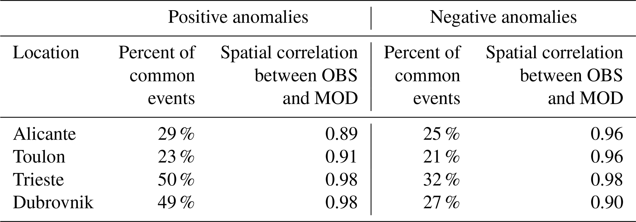
Figure 2 shows MSLP composites corresponding to large positive SLAs. Each map results from the average of the 6-hourly ERA-Interim MSLP fields that are closest to the time of the 100 largest peak of independent SLAs, considering the OBS (left column) and MOD lists (right column). In both columns the MSLP composites show the presence of cyclones. Trieste and Dubrovnik exhibit similar synoptic patterns, have a large number of events common to the MOD and OBS lists (50 % and 49 % in the Table 1) and have the highest value of spatial correlation (0.98) between the corresponding MSLP composites. Slightly lower values of correlation, 0.89 and 0.91, and a smaller number of common events, 29 % and 23 %, occur at Alicante and Toulon, respectively. These correlation values are computed between the MOD and OBS MSLP composite including all grid points within a distance of 20 grid steps from the station. Autocorrelation within a MSLP field is high and the estimate of the actual degrees of freedom would be required for assessing the significance of these correlation values. Performed tests show that significance remains above the 95 % confidence level even if a degree of freedom as low as 20 is assumed.

Figure 3 shows MSLP composites corresponding to large observed and modelled negative SLAs. For negative SLAs values of spatial correlation between MOD and OBS composites are also large (never lower than 0.90). The number of events common to the two lists is lower for negative than for positive SLA, correspondingly suggesting larger errors in the hindcast than for positive SLAs. Note that the composites of Alicante and Trieste report the presence of a cyclone over the Mediterranean Sea in association with negative SLAs as well.

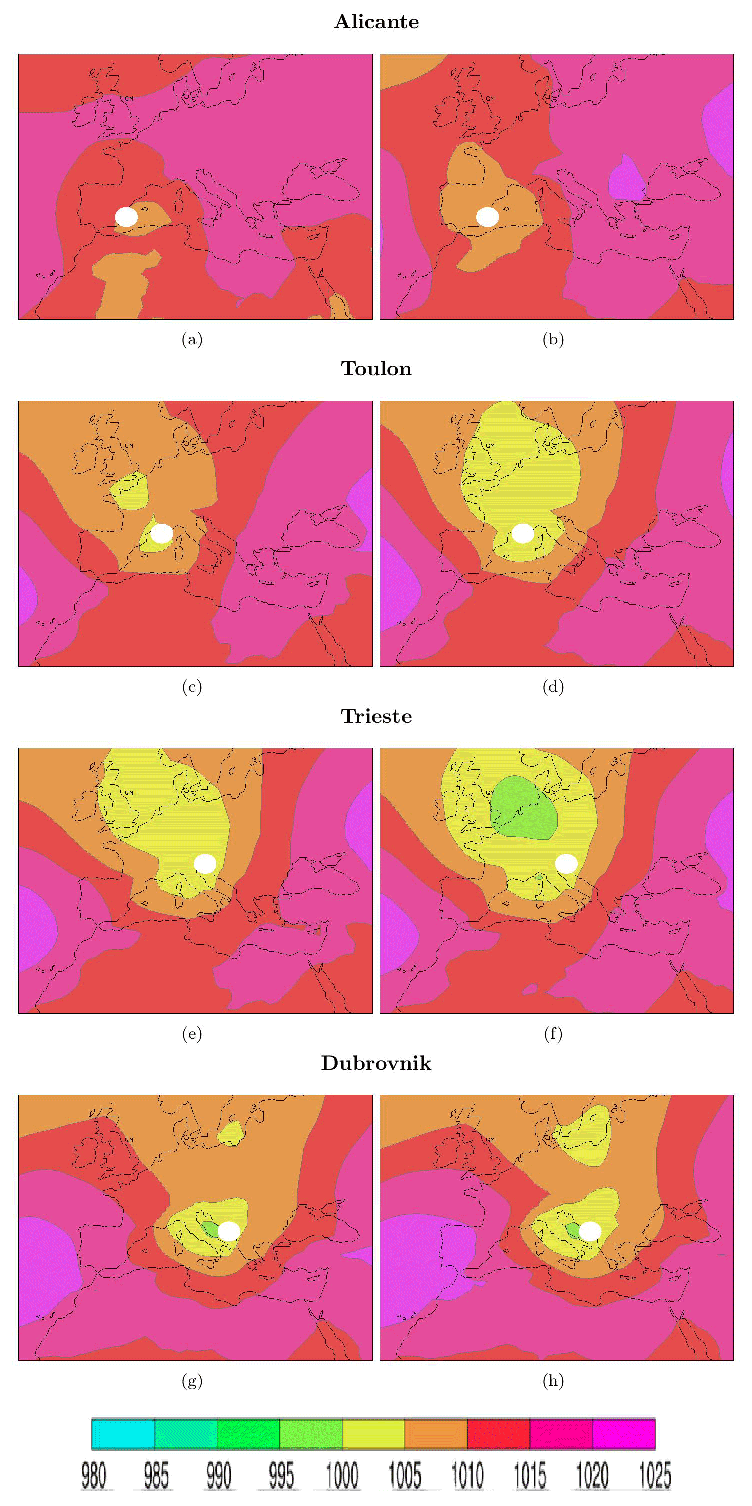
Figure 2Composite of ERA-Interim SLP fields (values in hPa) associated with large positive sea level anomalies in Alicante (a, b), Toulon (c, d), Trieste (e, f) and Dubrovnik (g, h), denoted with white circles in the maps. The right and left column show composites based on the COSMO-ERA hindcast (MOD) and in the observed time series (OBS), respectively. Each composite is based on a total number of 100 events, obtained by selecting the largest events in the 1979–2001 period.

In general, cyclones are deeper and better defined in the MOD composites than in the OBS composites. Actually, if SLAs are extracted from the model hindcast, the model simulation ensures a strong consistency between the MSLP fields (contributing to the MOD composites) and SLAs. If SLAs are extracted from observed time series, the corresponding MSLP (contributing to the OBS composite) might incorrectly reproduce the real position and the intensity of the cyclones because of errors in the ERA-Interim reanalysis and in the COSMO-ERA hindcast.

The similarity between the two columns of Figs. 2 and 3 show that the MSLP pattern associated with large positive SLAs in the model simulation is accurate and realistic, in spite of inaccuracies in the simulated maxima of individual events. Consequently, we conclude that the MSLP composites based on simulated events realistically reproduce the atmospheric patterns leading to large SLAs.

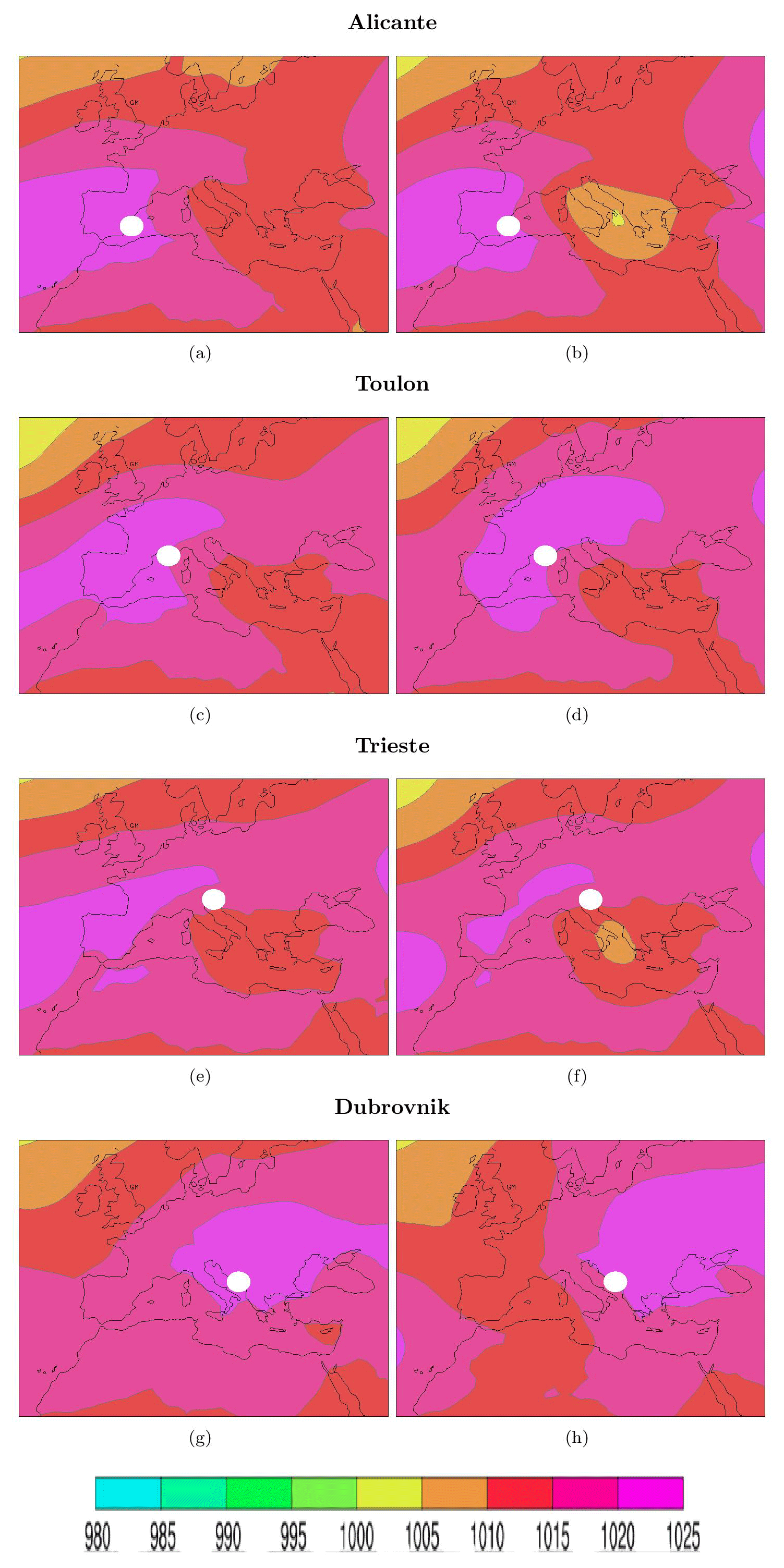
Figure 3The same as Fig. 2 but for large negative anomalies.

3.2 Evolution of the MSLP field during the development of large sea level anomalies

Figures 4 and 5, based on the 100 largest positive and negative SLA, respectively, show the ERA-Interim MSLP composites 48 h before (left column), 24 h before (middle column) and at the time (right column) of the SLA maxima. Each line of Figs. 4 and 5 separately considers one of the nine coastal stations. Figure 4, which considers positive SLAs, shows the presence of a cyclone, which is consequently a permanent feature in the atmospheric circulation leading to large positive SLAs. Figure 5, which considers negative SLAs, also shows the presence of a cyclone in the basin for most stations, except for Dubrovnik, Thessaloniki and Tripoli.

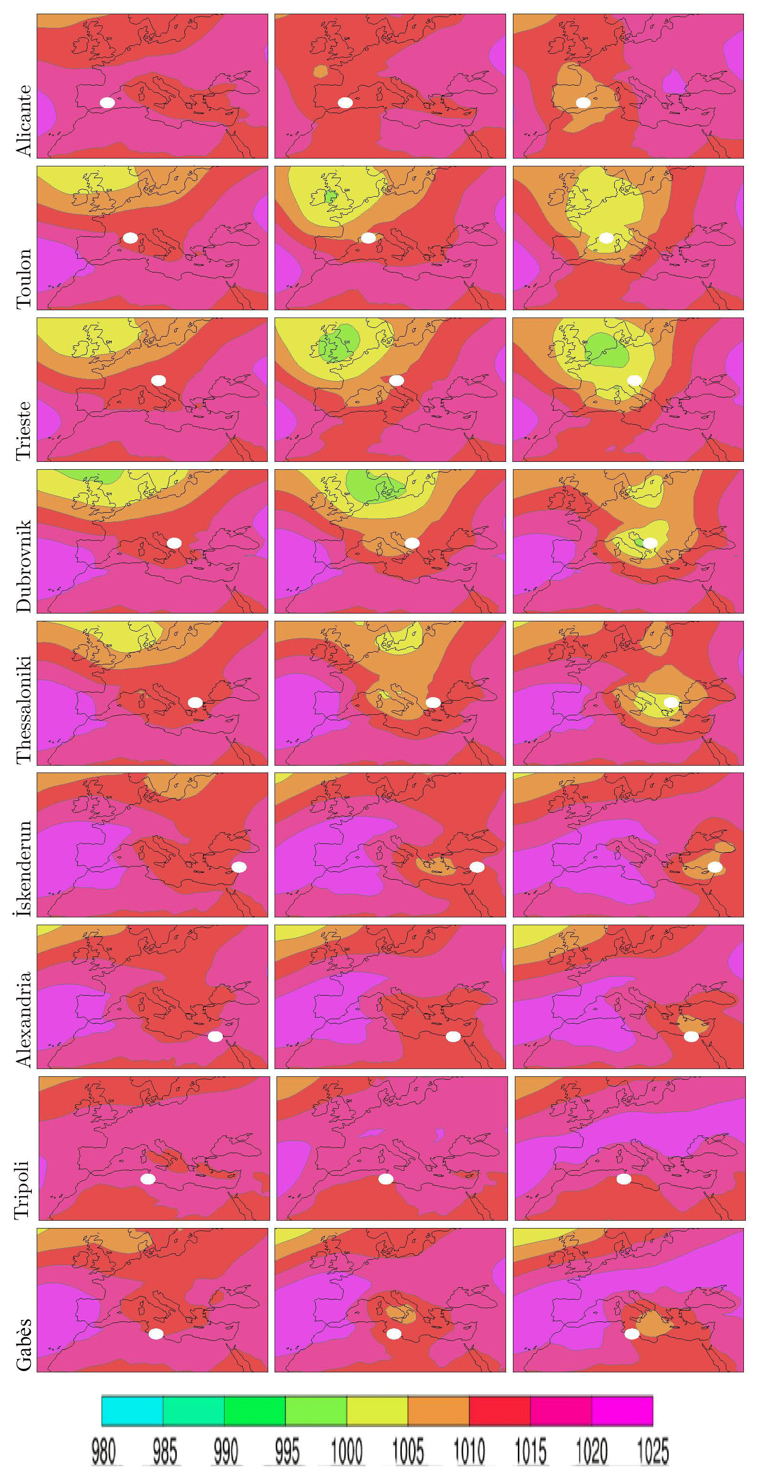
Figure 4Composites of ERA-Interim MSLP fields (in hPa) associated with the values of large positive sea level anomalies 48 h before (left column), 24 h before (middle column) and at the peak (right column) of the event in Alicante, Toulon, Trieste, Dubrovnik, Thessaloniki, İskenderun, Alexandria, Tripoli and Gabès, denoted with white circles in the maps.

Locations along the northern coastline (Toulon, Trieste, Dubrovnik, Thessaloniki) for positive SLAs and, to a lesser extent, along the southern coastline for negative SLAs (İskenderun, Alexandria, Gabès) evidence a western Mediterranean cyclogenesis triggered by the passage of a deep MSLP minimum over central Europe. In the latter three cases the presence of a cyclone in the western MR is associated with a eastward pressure gradient and high pressure over the eastern MR. Cyclones producing positive SLAs in the Levantine basin (at İskenderun, Alexandria and Tripoli) move along the southeastern part of the Mediterranean storm track (see Fig. 1 of Lionello et al., 2016) after having been generated in the northwestern part of the basin. The evolution of a cyclone moving along the northwestern Mediterranean storm track is also evident for negative SLAs in the northwestern MR (Alicante, Toulon, Trieste). For these three stations, the presence of a cyclone in the eastern MR is associated with a westward pressure gradient and a high pressure in the western MR. For negative SLAs at İskenderun and Alexandria in the eastern MR the cyclone centres remain in the western MR, not far from cyclogenetic areas close to the Iberian peninsula, with a eastward pressure gradient associated with a high pressure in the eastern MR. Composites of negative SLAs at Dubrovnik, Tripoli and Thessaloniki show a persistent high pressure over a large part of the basin during the event without the presence of a cyclone inside the MR. For negative SLAs in Gabès (and to a lower extent in Trieste) the position of the cyclone is such to produce a strong offshore wind blowing over shallow water areas.

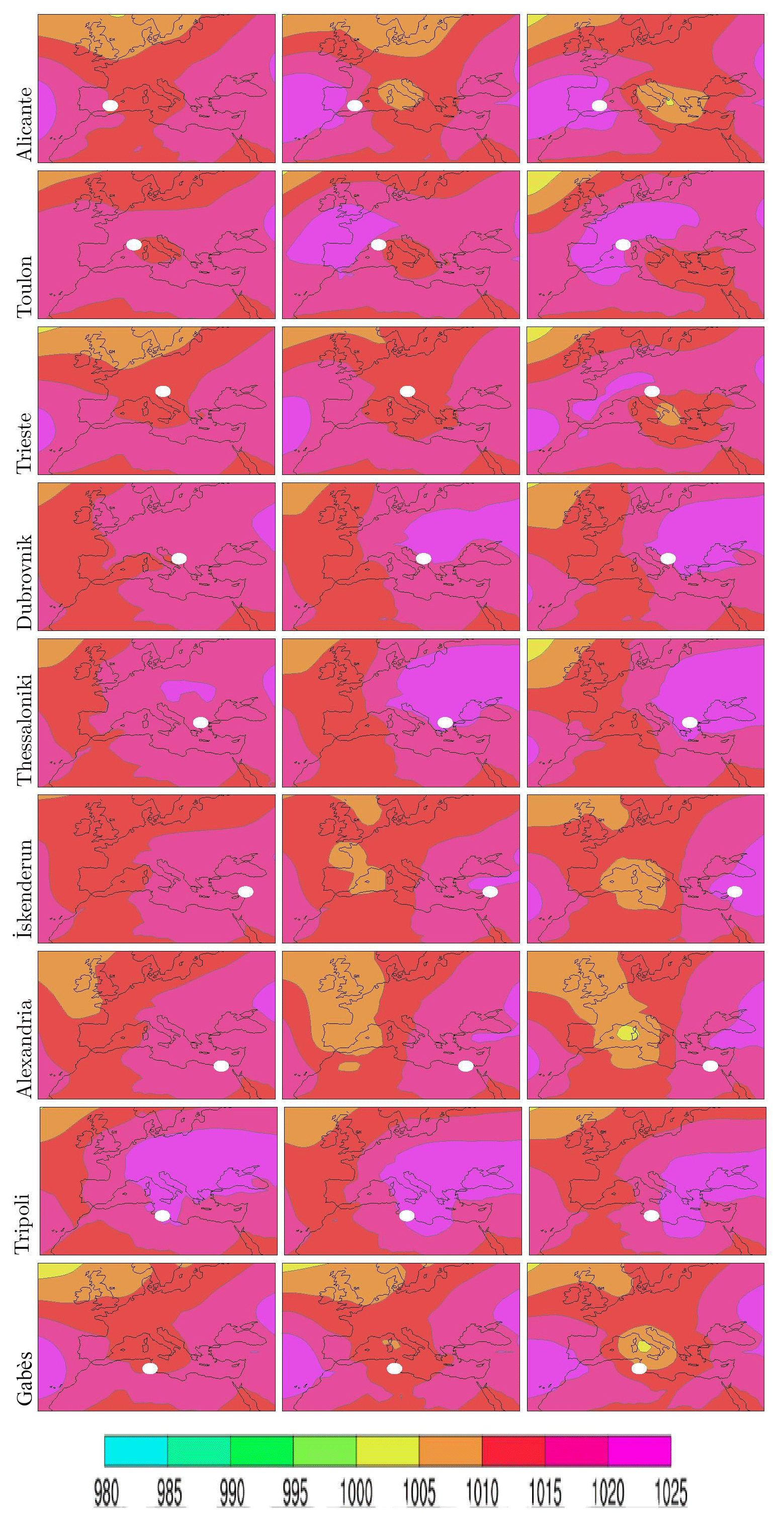
Figure 5The same as Fig. 4 but for large negative sea level anomalies.

3.3 Cyclone tracks associated with large sea level anomalies

To assess the link between the presence of a cyclone and large SLAs, the procedure adopted by Reale and Lionello (2013) for associating cyclones and precipitation extremes has been adapted to storm surges and applied to the ERA-Interim MSLP fields. The procedure consists of a sequence of steps: a MSLP minimum is searched within a radius of 20^∘ from the considered coastal station in the 6-hourly field, whose time is closest to the time of maximum amplitude of each positive and negative SLA event. If only one minimum is found the corresponding cyclone is associated with the event. If more than one minimum is present inside the search radius, the closest minimum is selected. When no minimum is found the event is not assigned to any cyclone.

Figure 6 shows the density tracks of cyclones associated with large positive SLAs and the positions of the cyclone centres at the peak of the events (blue squares). Density is computed splitting the domain in cells of 1.5^∘ size and counting the cyclone centres located within each cell as each cyclone moves along its track. The units used are probability per square kilometre. Each panel refers to a different coastal location (red square). It is evident that cyclone tracks initiate in the well-known cyclogenetic areas located inside and around the Mediterranean Sea (North Africa, south of the Atlas Mountains, Gulf of Genoa, Adriatic Sea, Cyprus area, Black Sea area) and in the northeastern Atlantic (H.M.S.O., 1962; Alpert et al., 1990; Trigo et al., 1999, 2002; Maheras et al., 2001; Lionello et al., 2002, 2016; Garcies and Homar, 2011; Nissen et al., 2010; Campins et al., 2011; Reale and Lionello, 2013). The prevalent motion of the cyclone centre is southeastwards along the Mediterranean branch of the Mediterranean storm track. The importance of Atlantic cyclones decreases as the coastal station location moves eastwards while the importance of cyclogenesis over the Mediterranean Sea simultaneously increases, shifting towards the Levantine basin for the most southeastern stations (İskenderun and Alexandria). Cyclones that originated over North Africa are particularly relevant for Tripoli and Gabès and join the Mediterranean storm track in the eastern Mediterranean. In most cases, cyclone centres at the time of the SLAs are located so that the associated flow is directed towards the coast. In fact, the wind contributes a fraction of SLA in all locations but it is the dominant factor only in locations that are characterised by a long shallow water fetch, i.e. mainly Trieste and Gabès (Conte and Lionello, 2013), producing, depending on its direction with respect to the shore, a set-up or set-down effect.

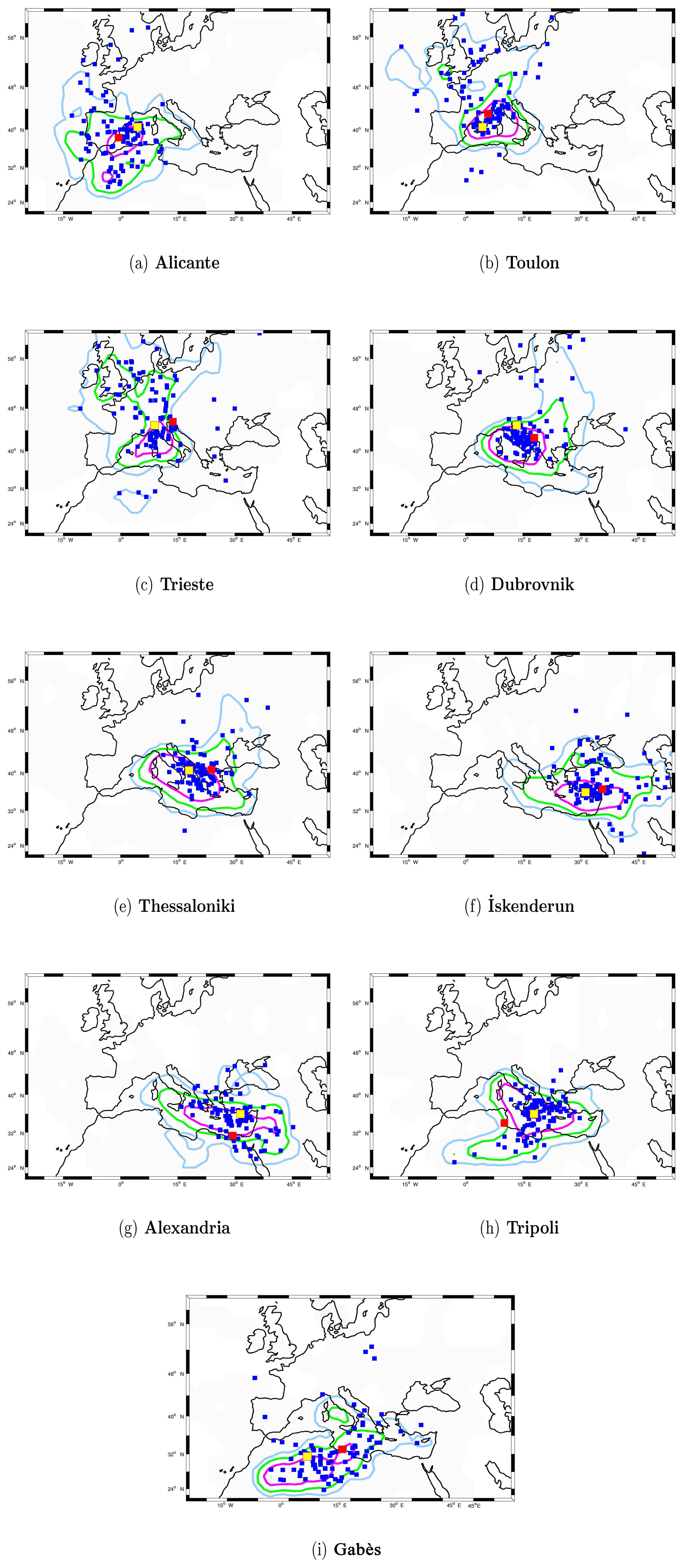
Figure 6Track density of cyclones producing large sea level anomalies at Alicante (a), Toulon (b), Trieste (c), Dubrovnik (d), Thessaloniki (e), İskenderun (f), Alexandria (g), Tripoli (h) and Gabès (i) (locations are denoted with a red square). Blue squares show the position of the cyclone centres at the peak of the sea level anomaly. The yellow squares denote the reference position used in Table 2 and Sect. 3.4. A smoothing radius of 5^∘ is applied to the original data resolution (1.5^∘). Contour lines are drawn at the $\mathrm{25}\times {\mathrm{10}}^{-\mathrm{7}}$ (blue line), $\mathrm{0.5}\times {\mathrm{10}}^{-\mathrm{7}}$ (green line) and 1$\times {\mathrm{10}}^{-\mathrm{7}}$ (magenta line) levels. The units used are probability per square kilometre.

Figure 7 shows the track density and cyclone positions for negative SLAs and relevant differences with respect to positive SLAs. In some stations (Toulon, Trieste, Tripoli and Gabès) the cyclones centres are concentrated in positions that determine a wind blowing offshore at the time of the negative SLAs (wind set-down), while in other stations the cyclone centres are broadly distributed with several accumulation areas. Note that, at the time of the negative SLA event for Trieste and Gabès, the cyclones are close to the station, while in other cases (such as Toulon, Alicante, Tripoli, Dubrovnik and Thessaloniki) they are positioned over the part of the Mediterranean basin opposite of where the event occurs. In the two former stations, the negative SLA is caused by the wind set-down. In the latter stations, the location of the cyclone is consistent with the prevalence of high-pressure conditions in the location where negative SLAs occur, which is related to the cyclone centre through a strong MSLP gradient across the basin (see also Sect. 3.5).

Figure 7The same as Fig. 6, except referring to large negative sea level anomalies and to Table 3.

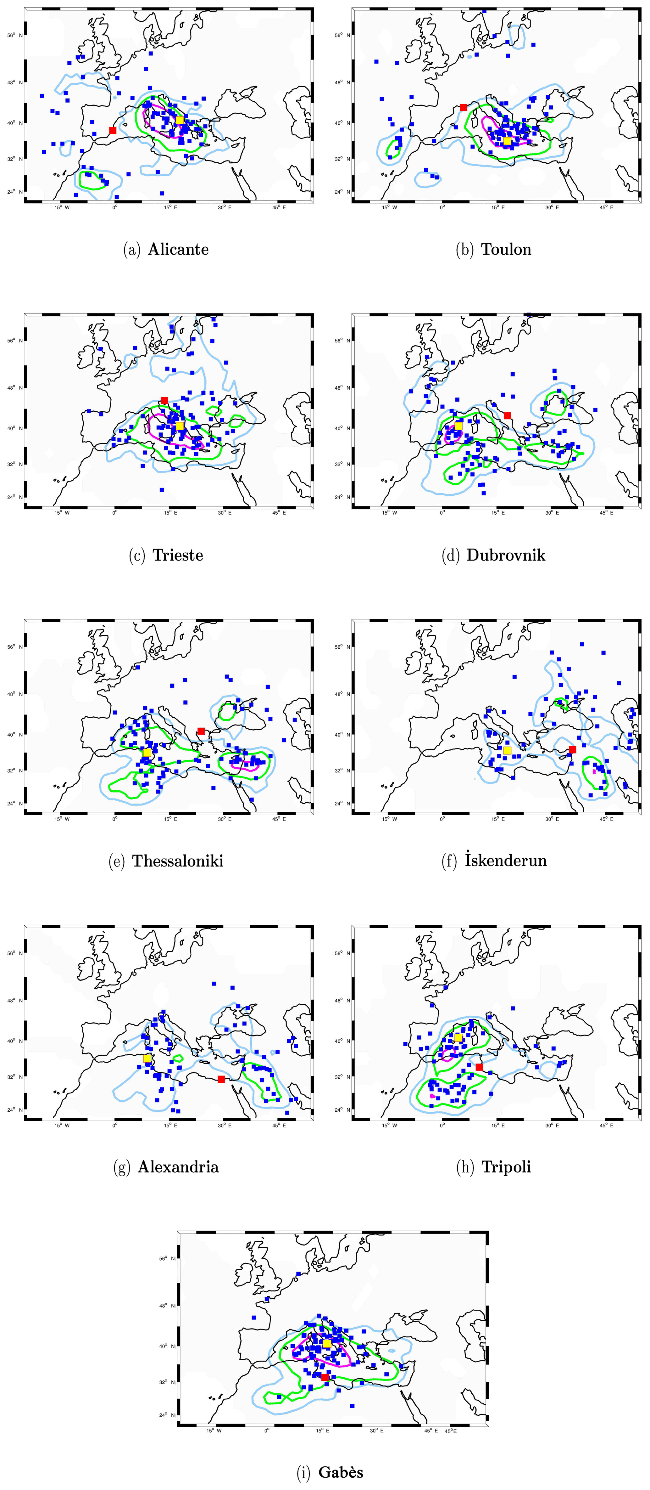
Cyclone track densities in Figs. 6 and 7 evidence the Mediterranean storm track, along which most cyclones move after having been originated inside the Mediterranean. Differences are visible in the signature of cyclones entering the Mediterranean Sea from North Africa (northeastern Atlantic) that are the stronger (weaker) in Fig. 6 than in Fig.7. Comparing Fig. 6 and 7 we infer that the same cyclone can eventually be associated with positive and negative SLAs in different parts of basin. For example, the tracks of cyclones associated with negative SLAs in Alicante, Toulon and Trieste are similar to those associated with positive SLAs in Thessaloniki, showing that the same cyclone, when moving along the main branch of the Mediterranean storm track, can produce negative SLAs at the former stations and positive at the latter.

Figure 8The same as Fig. 6, except referring to large negative sea level anomalies, the presence of anticyclones and Table 4.

3.4 Statistics of cyclone centre positions during large sea level anomalies

In this subsection we investigate to which extent the positions of the cyclone centres at the time of the positive and negative SLAs (Figs. 6 and 7) are statistically linked to the events themselves. This is analysed by computing the probability (relative frequency) that a cyclone is present within a 10^∘ radius from the reference position, which is denoted with the yellow square, and comparing it to the background “climatological” probability. The latter is estimated by searching for cyclone centres in a sequence of MSLP fields extracted with a time step of 10 d (to avoid correlations among successive fields). If the difference between the two values is significant (the t test of the mean with a significant level of 95 % has been used), then the presence of the SLA is statistically linked to the position of the cyclone in an area surrounding the reference position. The reference position is the centre of the 5^∘ wide latitude–longitude cell, where the density of cyclone centres (blue squares in Figs. 6 and 7) has a maximum. This procedure is repeated for each station. For negative SLAs at İskenderun, where this criterion would locate the reference at the eastern boundary of the map, the second largest maximum (in the middle of the Ionian Sea) has been used.

Further, for each cyclone associated with positive and negative SLAs the cyclogenesis point (where its trajectory starts) has been identified and attributed to four areas: Atlantic (Atl), North Africa (Afr), western Mediterranean (WM), eastern Mediterranean (EM) and Asia–Europe (AsEu), according to the main cyclogenetic areas that are suggested by the existing literature (e.g. Lionello et al., 2016 and Fig. 1).

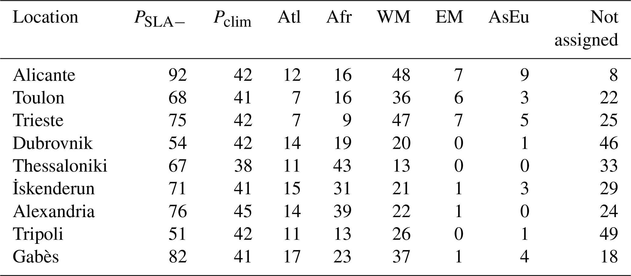
Table 2 compares the probability that a cyclone is around the reference position for positive SLA (column P_SLA+) with the climatological probability (column P_clim). Each line denotes a different station. At all stations, differences are statistically significant at the 95 % level. Results show that for all stations the probability of finding a cyclone around the reference position in coincidence with a positive SLA is higher than the climatological mean.

Further, Table 2 reports the relative frequency of cyclogenesis in the four different areas. The most important cyclogenesis areas is the WM for all stations, except for İskenderun and Alexandria, where it is the EM, and Tripoli, where it is Afr. Afr is also an important cyclogenetic area for Gabès (and it also plays an important role for Alexandria and İskenderun). Atl is only an important source of cyclones for stations located in the western Mediterranean (Alicante, Toulon, Trieste). The tracking algorithm failed to find a cyclone within a 10^∘ radius from the reference position with comparatively large frequency in Gabès (37 %), Toulon (29 %), Alicante (28 %) and Trieste (25 %).

The link with cyclones is statistically significant for all stations for large negative SLAs as well (Table 3). However, the percentage of “not assigned” events is generally higher than for positive SLAs and it is particularly large for Dubrovnik and Tripoli, where almost 50 % of large negative SLAs occurred when no cyclone was present within a 10^∘ radius from the reference position. This is actually consistent with the MSLP composites in Fig. 3.

The cyclogenesis areas that have been identified for positive SLA are confirmed but for negative SLAs their relative importance is different (Table 3). With respect to positive SLAs, the frequency of Atl cyclogenesis is more important for negative SLAs in the eastern Mediterranean than in the western Mediterranean. Considering large negative SLAs, the WM keeps a leading role, being the main overall source and individual sources for most stations (Alicante, Toulon, Trieste, Dubrovnik, Tripoli and Gabès), while very few cyclones are generated in the Ë and Afr is the main cyclogenesis area for Alexandria and İskenderun.

Table 2Statistics of cyclones producing the 100 largest positive sea level anomalies in each considered station. The first two columns, labelled “P_SLA+” and “P_clim”, report the probability (%) of finding a cyclone within a 10^∘ search radius from the reference point (denoted with a yellow square in Fig. 6) at the time of the event and the corresponding climatological mean value, respectively. Differences between the P_SLA+ and P_clim values are statistically significant at the 95 % level. The following columns (labelled Atl, Afr, WM, EM, AsEu) report the probability (%) that the cyclogenesis of the cyclone associated with the event occurred in the areas shown in Fig. 1. The last column reports the number of events in the period 1979–2001 that were not assigned to any cyclone.

Download Print Version | Download XLSX

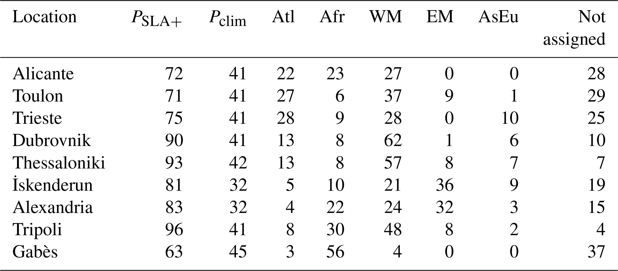
Figure 8 shows the centres of anticyclones at the time of negative SLAs. It is made following the same procedure that was used for Fig. 7, which refers to cyclones. It reveals the location of centres of anticyclones in the areas where the right column of Fig. 5 shows high-pressure systems. Anticyclones are actually concentrated around the stations, with the exception of Gabès and, to a lesser degree, Trieste, where the wind effect is much larger than the inverse barometer effect and anticyclones play a minor role. Therefore, negative SLAs are linked to the presence of a high pressure around the station. This is necessarily true for most stations because of the inverse barometer effect. However (see Table 4), the probability to find an anticyclone at a distance lower than 10^∘ from the reference position³ at the time of negative SLAs is significantly larger than the climatological value only for three stations (Toulon, Thessaloniki, İskenderun). On the contrary, in Gabès, the absence of an anticyclone is linked to negative SLAs (and this is justified by the dominant role of the wind at this station). The link with the presence of a cyclone in the part of the basin opposite to the station (Table 3) is stronger than what is shown in Table 4 for anticyclones.

Table 3Same as Table 2 except it refers to negative sea level anomalies.

Download Print Version | Download XLSX

3.5 The link of the SLA values with cyclone positions and intensities

Here we investigate the SLAs at the nine considered stations as function of the position of cyclones inside the MR. Each panel in Fig. 9 considers a different coastal station and shows the mean SLA at the selected station as function of the position of the cyclone centre. Each panel has been obtained dividing the MR in 1.5${}^{\circ }\times \mathrm{1.5}$ latitude–longitude cells, selecting the time when a cyclone centre is within each cell, extracting from the time series the corresponding SLA values at the considered station, computing their average and attributing it to the cell. Note that these average SLAs result from cyclones of different intensities and structures, with some of them eventually being very shallow.

Table 4The same as Table 2 except that it refers to negative sea level anomalies; the presence of anticyclones and the columns with information on the genesis of the anticyclones are not reported. The columns, labelled “$P_{\mathrm{SLA}-}^{\mathrm{A}}$” and “$P_{\mathrm{clim}}^{\mathrm{A}}$”, report the probability (%) of finding an anticyclone within a 10^∘ search radius from the reference point (denoted with a yellow square in Fig. 8) at the time of the event, the corresponding climatological mean value and of failing in detecting the presence of an anticyclone, in this order. Bold values denote differences between $P_{\mathrm{SLA}-}^{\mathrm{A}}$ and $P_{\mathrm{clim}}^{\mathrm{A}}$ that are statistically significant at the 95 % level.

Download Print Version | Download XLSX

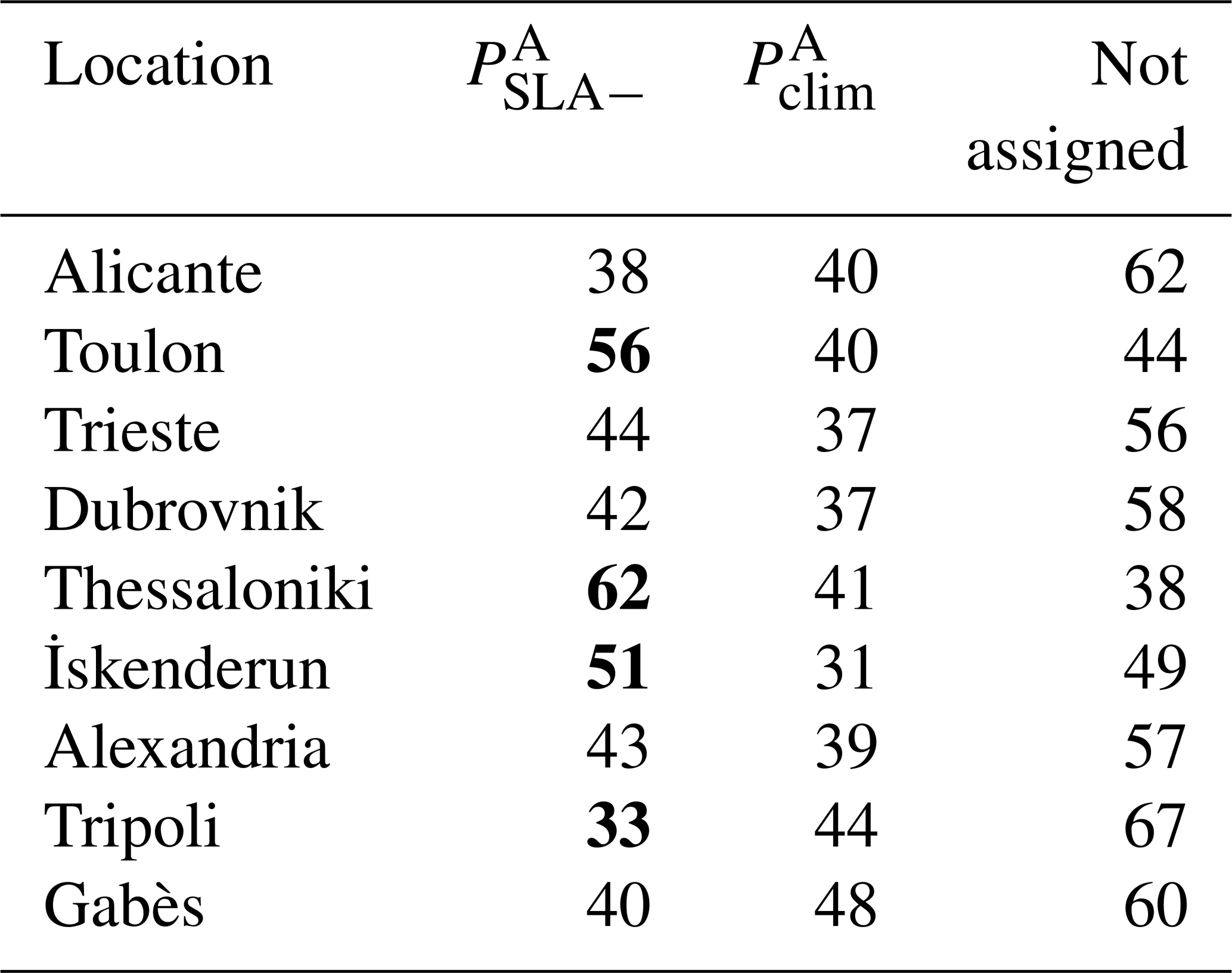
Figure 9 allows us to distinguish between local and remote effects associated with the passage of cyclones. The inverse barometer effect caused by the low-pressure values around the centre of the cyclones is shown by the positives SLA values in the area surrounding the stations (which is particularly intense in Trieste, Dubrovnik and Thessaloniki). The wind set-up is shown by positive (negative) values in the areas where the cyclone centre would cause a wind, pushing water masses toward (away from) the coastal station. In general, the shift of the areas with positive or negative values with respect to the station is evidence of the importance of the wind set-up component, which is large in the presence of a shallow water fetch. The role of the wind set-up is particularly evident in Gabès (Fig. 9i), where cyclones located above North Africa (west of the Strait of Sicily) produce positive (negative) SLAs, and the inverse barometer effect is negligible in comparison. The situation in Tripoli is analogous to Gabès.

In almost all panels of Fig. 9 significant negative values are present in areas of the basin relatively far away from the stations, at a distance that is too large to be a direct action of the wind and low pressure of cyclones on the sea level. Two examples are the westernmost (Alicante) and easternmost stations (and Alexandria), where negative SLAs are associated with a cyclone above the central Mediterranean. In these cases, the presence of a cyclone is associated with a pressure gradient across the basin (see Fig. 10), producing a redistribution of mass and a temporary decrease in sea level in areas far away from the cyclone centre. However, in Fig. 9, positive features are larger than negative features, meaning that the association between SLAs and cyclone positions is larger for positive than for negative events.

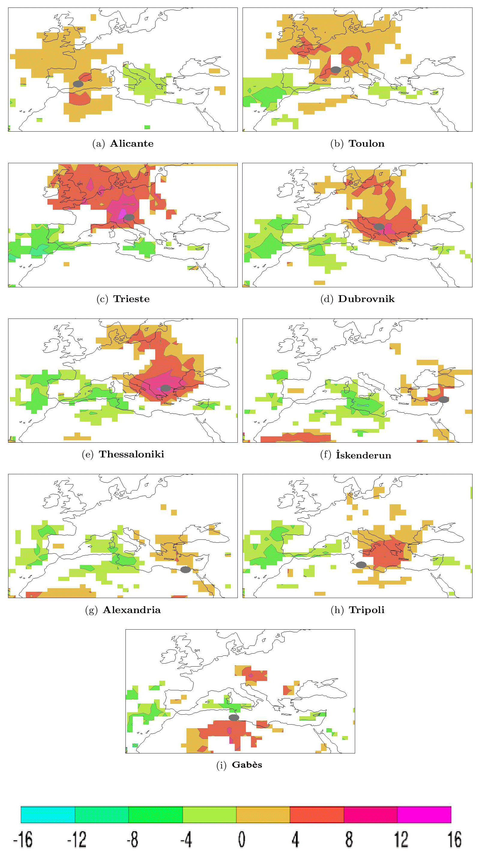
Figure 9Mean SLA (cm) at the coastal station as a function of cyclone positions. Each panel considers a different coastal station: Alicante (a), Toulon (b), Trieste (c), Dubrovnik (d), Thessaloniki (e), İskenderun (f), Alexandria (g), Tripoli (h), Gabès (i). Only values reaching the 90 % significance level are shown.

The link between MSLP anomaly at the coastal station and position of the cyclone is shown in Fig. 10. This figure has been obtained following exactly the same procedure as Fig. 9, except it plots the difference in MSLP between the station and the cyclone centre (and not the SLA). The small values around the position of each coastal station are the obvious consequence of the cyclone centre being close to the station. The positive values, between 10 and 15 hPa in the areas of the basin opposite to the station evidence that when the cyclone centre is located in such areas, the pressure at the station is high and the inverse barometer effect contributes to negative sea level anomalies.This happens at Alicante, Toulon, Thessaloniki and Trieste when a cyclone is located in areas where the density of cyclone centre in Fig. 7 is large. This explains, on the basis of the inverse barometer effect, the link between negative SLAs and the presence of a cyclone at a distance that is too large for its direct action on the sea level at the considered station, though other factors are involved (see Sect. 3.6).

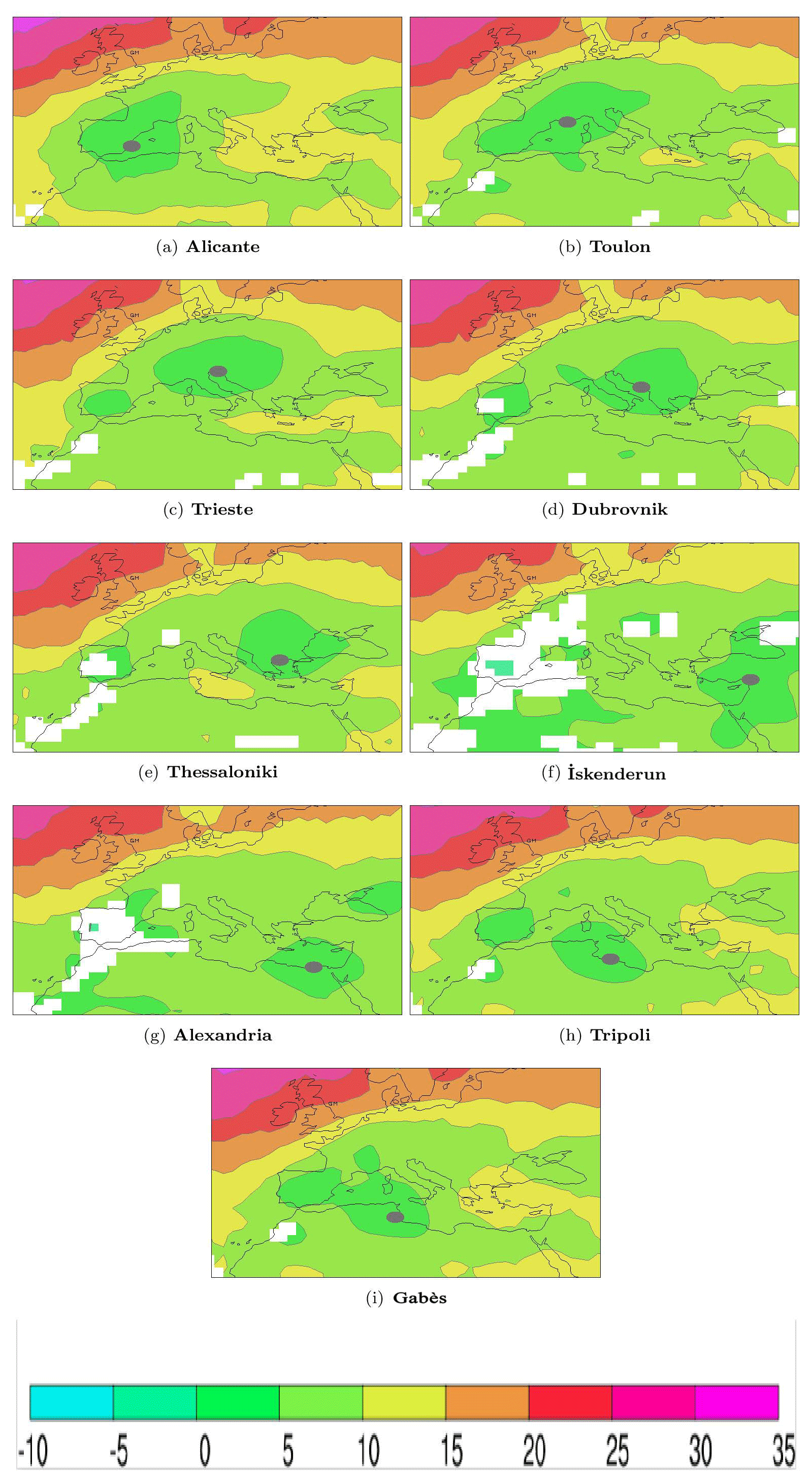
Figure 10Difference between MSLP (hPa) at the coastal station and cyclone pressure minimum as function of cyclone position. Each panel considers a different coastal station: Alicante (a), Toulon (b), Trieste (c), Dubrovnik (d), Thessaloniki (e), İskenderun (f), Alexandria (g), Tripoli (h), Gabès (i). Only values reaching the 90 % significance level are shown.

The dependence of the SLA value on the cyclone MSLP central minimum is analysed by computing the linear regression coefficient between the SLAs and the values of the MSLP minima. Each panel of Fig. 11 considers a different coastal station and adopts a procedure similar in part to Fig. 9. The whole MR has been divided in 1.5${}^{\circ }\times \mathrm{1.5}$^∘ latitude–longitude cells. When a cyclone centre is within a cell, the paired MSLP minimum and corresponding SLA anomaly at the coastal station is selected. For each cell the regression coefficient of SLA values with respect to MSLP minima has been estimated and plotted in Fig. 11 as a function of the cyclone centre position. Therefore, each panel of Fig. 11 is meant to show the sensitivity of the SLA at the considered station on the cyclone central MSLP minimum as a function of the cyclone position. Only values above the 90 % confidence level are shown. Since SLA increases for decreasing value of pressure minima, in Fig. 11 the orange–red colours denote negative regression coefficient values (this is meant to facilitate the comparison with Fig. 9).

The inverse barometer effect would produce a value of −1 cm hPa⁻¹ when a cyclone centre is exactly above the station. However, the regression coefficients not only directly reflect the inverse barometer effect (which is a local relation) but also the contribution of wind or other dynamics to the SLAs. When the cyclone centre is located away from the station the contribution of the inverse barometer effect decreases because of the decreasing amplitude of the MSLP anomaly with the distance from the cyclone centre. On the contrary, the importance of the contribution due to the wind set-up might increase if the position of the cyclone centre establishes an atmospheric circulation, accumulating water masses against the coastal station (or subtracting them from it). Trieste (Fig. 11) clearly shows that the dependence of the positive SLA on the intensity of the cyclones is largest when their centres are located in the gulf of Genoa, in the position such that the associated wind blowing along the Adriatic Sea will accumulate water on its northern shore.

In fact, the regression coefficients link MSLP minima and SLA values in locations that are separated by several hundreds of kilometres. The largest statistically significant values of regression coefficients have been found at a distance of approximately 700 km from the station for Trieste (−2.2 cm hPa⁻¹), Gabès (−1.7 cm hPa⁻¹), Thessaloniki (−1.6 cm hPa⁻¹) and İskenderun (−1.5 cm hPa⁻¹). Values at other stations are smaller in module (less than −1.2 cm hPa⁻¹). However, these regression coefficients cannot be used for estimating extreme SLAs, when the impact of the atmospheric forcing is amplified by peculiarity of the atmospheric pattern.

Figure 11 provides statistical evidence of a teleconnection⁴ linking negative SLAs to cyclones with centres that are located thousands of kilometres from the station. The yellow areas far away from the stations in Fig. 10 show that a cyclone positioned in those areas is linked to negative SLAs at these two stations. Therefore, this figure clearly shows the connection between intensity of cyclones in the opposite part of the basin and negative anomalies at İskenderun and Alexandria.

The patterns in Figs. 9 and 11 are consistent with the geographical distribution of cyclone centres in Figs. 6 and 7. The correspondence is not exact but this should be expected. In fact, Figs. 6 and 7 include only the largest SLA events while Fig. 9 represents the mean SLA response to all cyclones that crossed the MR during the hindcast.

Figure 11Linear regression coefficient (cm hPa−1) of SLAs at the coastal stations versus MSLP cyclone minima as function of the cyclone centre position. Each panel considers a different coastal station: Alicante (a), Toulon (b), Trieste (c), Dubrovnik (d), Thessaloniki (e), İskenderun (f), Alexandria (g), Tripoli (h), Gabès (i). Only values significant at the 90 % confidence level are shown.

3.6 Dynamics of sea level anomalies in the Mediterranean Sea

Figures 12 and 13 show the features of the SLAs over the whole Mediterranean Sea. Each panel is a composite of the fields corresponding to the 100 largest SLA maxima at each of the nine coastal stations considered in this study. Figures 12 and 13 consider positive and negative SLAs, respectively. The four columns show the total SLA (first column, cm), the contribution due to the inverse barometer effect (second column, %) and the residual (third column, %), meaning the difference between the first and the second column, which represents the part of SLA that is not explained by the inverse barometer effect. The fourth column shows the composites of the wind fields at the time of the SLAs largest amplitude. The maps displaying the inverse barometer and residual contributions show normalised values, obtained by dividing by the SLA maximum (minimum) of the total positive (negative) corresponding SLA map (in other words, the units used are percentages of overall maxima and minima). The inverse barometer contribution is built using the 6-hourly MSLP of the COSMO-ERA dataset closest to the time when the SLA has the largest magnitude at the coastal station.

The presence of a cyclone at the time of the positive SLA event is shown by the shape of the SLA associated with the inverse barometer effect, which mimics the contour lines around a cyclone centre. In the case of positive SLA (Fig. 12), the distance between the station and the maximum of the inverse barometer effect (central column) is an indication of the importance of the wind (particularly large for Gabès), which is made evident by a local and large SLA in the area around the station in the maps of the residual (right column).

The presence of a cyclone is also evident in the composites of negative SLAs (Fig. 13, values are negative because they are normalised using the SLA minimum), with the exception of Dubrovnik. However, in these cases, the cyclone centres are located in the opposite part of the basin with respect to the position of the stations. Several different dynamics are suggested by these maps. At Tripoli, Alexandria, İskenderun and Thessaloniki the presence of a cyclone is associated with a pressure gradient across the basin such that the inverse barometer effect contributes substantially to the negative SLA in the position of the station. For Gabès and Trieste, where there is a long shallow fetch, the atmospheric circulation around the cyclone centre produces a set-down at the station, which is shown by the locally large contribution to the negative SLA in the area around the station in the maps of the residual (right column).

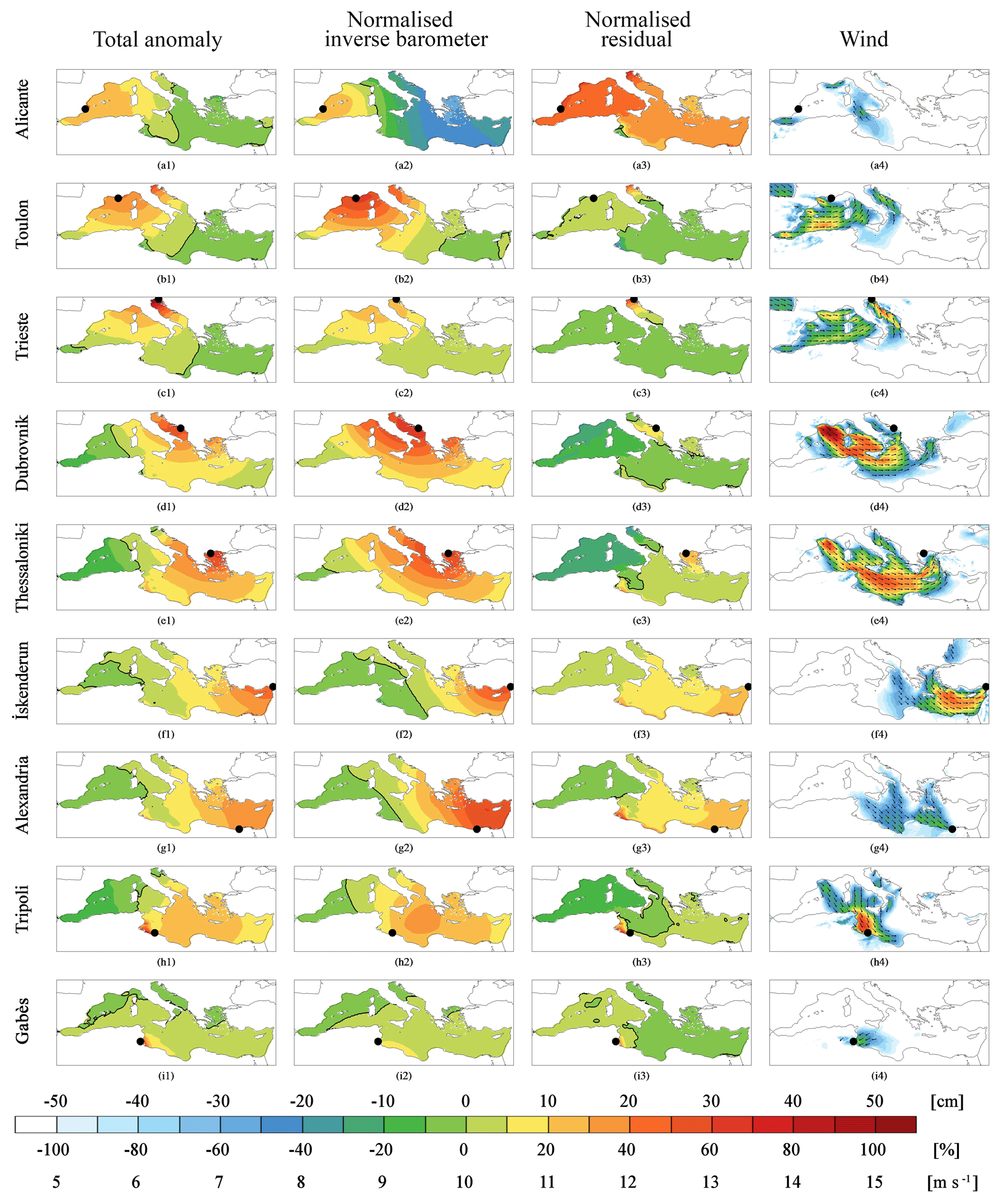
Figure 12Composites of sea level anomalies and wind fields at the time of positive SLAs at the nine stations considered in this study: Alicante, Toulon, Trieste, Dubrovnik, Thessaloniki, İskenderun, Alexandria, Tripoli, Gabès (from top to bottom in this order). The first column reports the total anomaly (cm, upper annotation along the colour bar), the second column reports the contribution due to the inverse barometer effect and the third column reports the residual. Values in the second and third column are normalised with the maxima of the total SLA in the first column (%, first line of annotation below the colour bar). The thick black line denotes the zero level contour. The fourth column shows the wind field (m s⁻¹, lowest annotation below the colour bar, values below 5 m s⁻¹ are masked). Arrows that show the wind direction are drawn every 1.25^∘ and only for values larger than 7.5 m s⁻¹.

Some stations show a large residual that, because of its extension, cannot be associated with the action of the wind and it reflects a contrast of level between the western and eastern parts of the Mediterranean Sea. In some cases, such as Alicante, Toulon, İskenderun and Tripoli, it produces a very substantial contribution to the magnitude of the SLA, particularly when it is negative. This contribution amplifies the contrast of sea level between the western and eastern part of the Mediterranean that is already produced by the difference of MSLP associated with the presence of a cyclone inside the basin. This suggests that, in the model simulations, during the synoptic system evolution, the SLA has no sufficient time to reach equilibrium with the MSLP field and the Gibraltar strait does not allow sufficient water flow to comply with the inverse barometer effect. In practice, during the development of both positive and negative SLAs at the coastal stations, the average SLA of the whole Mediterranean changes little, in spite of the forcing caused by the inverse barometer effect. Whether this is realistic or an artificial model feature remains to be investigated.

The action of the wind is evident in the fourth columns of Figs. 12 and 13, which show the composites of the wind fields at the time of the SLAs largest amplitude. In these maps, the presence of a strong wind blowing towards the coast (Fig. 12, positive SLAs) or offshore (Fig. 13, negative SLAs) is consistent with the large residuals at Trieste, Tripoli and Gabès. For positive SLAs the wind is also present in correspondence with the residuals (which are smaller than in the previous stations) at Alexandria, İskenderun and Thessaloniki.

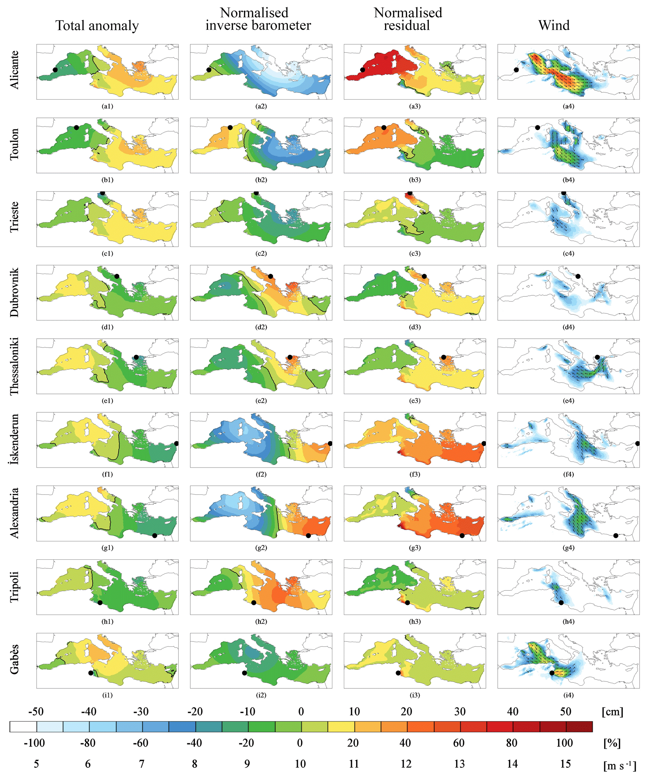
Figure 13The same as Fig. 12 except that negative sea level anomaly events are considered (in this case the minima of the SLA total in the first column are used for producing normalised values in the second and third column).