the Creative Commons Attribution 4.0 License.
the Creative Commons Attribution 4.0 License.
 | 05 Aug 2019
The effects of changing climate on estuarine water levels: a United States Pacific Northwest case study
Kai Parker
David Hill
Gabriel García-Medina
Jordan Beamer
Climate change impacts on extreme water levels (WLs) at two United States Pacific Northwest estuaries are investigated using a multicomponent process-based modeling framework. The integrated impact of climate change on estuarine forcing is considered using a series of sub-models that track changes to oceanic, atmospheric, and hydrologic controls on hydrodynamics. This modeling framework is run at decadal scales for historic (1979–1999) and future (2041–2070) periods with changes to extreme WLs quantified across the two study sites. It is found that there is spatial variability in extreme WLs at both study sites with all recurrence interval events increasing with further distance into the estuary. This spatial variability is found to increase for the 100-year event moving into the future. It is found that the full effect of sea level rise is mitigated by a decrease in forcing. Short-recurrence-interval events are less buffered and therefore more impacted by sea level rise than higher-return-interval events. Finally, results show that annual extremes at the study sites are defined by compound events with a variety of forcing contributing to high WLs.


Estuaries are important intersections of human and natural systems, serving as some of both the most resource-rich ecosystems on Earth and the most densely populated. Asked to meet many, at times conflicting, needs, estuaries require careful management. Unfortunately, coastal planning is limited by an insufficient understanding of how estuaries will respond to future conditions. In particular, extreme water levels (WLs) are of first-order importance, with flooding putting both lives and physical infrastructure at risk.
In the United States (US) Pacific Northwest (PNW), considerable progress has been made towards an understanding of hazard risk at open beaches as controlled by a combination of forcing drivers, including waves, tides, winds, and others (Barnard et al., 2014; Ruggiero, 2013; Serafin and Ruggiero, 2014). Flooding risk in PNW estuaries is less well understood, primarily due to the greater complexity of the estuarine environment. Research efforts have mostly focused on the Columbia River, which is societally important, but not necessarily characteristic of other PNW estuaries due to its large size and heavy damming and flow regulation (Jay et al., 2015, 2016; Lee et al., 2009). Estuarine hydrodynamics remain more complicated than open coastlines due to the additional driver of streamflow and a much more complicated topographical context (e.g., embayment and complex bathymetry) (Odigie and Warrick, 2018; Wahl et al., 2015). This makes estuaries difficult to simplify as they exhibit nonlinear water column response (Ding et al., 2013) with forcing contributions being difficult to uncouple (Wolf, 2009).
Consideration of future risk adds an additional challenge through a mismatch in timescales. Climate change signals are significant at scales of decades while individual extreme events occur at timescales of hours to days. This requires both high model temporal resolution and long model simulations. Long time series are additionally necessary for extreme value analysis and constraining event recurrence intervals (RIs). Balancing these needs with computational cost has remained a major obstacle and has led to a variety of modeling strategies. One approach takes advantage of the fact that extreme value analysis only requires information of the maxima events. Lin et al. (2012) use a unique approach based on multiple model complexities; an efficient model to determine which events will cause flooding and a more complex model to accurately quantify the dynamics of those events. As a second example, Orton et al. (2016) simply model the coastal responses to a large set of hurricane events. Both of these studies focus on the eastern US coastline where tropical cyclones are the principal driver of flooding events. Locations less dominated by tropical cyclones have a more diverse and balanced set of contributions to flooding (Parker, 2019). In these locations, extreme events can occur due to combinations of forcings which are not individually extreme, a phenomenon discussed in the literature as “compound events” (Gallien, et al., 2018; Leonard et al., 2014; Moftakhari et al., 2017b, 2019; Wahl et al., 2015). This makes it difficult to know a priori which events will result in maximum WLs.
Recent advances in computing power and parallel processing have opened up an alternative possibility of running continuous time series hydrodynamic models at climate change scales (decades to centuries). This allows examination of extremes without assuming which events will cause extremes. Additionally, a continuous time series analysis has other desirable properties. For example, an event-based approach limits analysis to only large RI events, eliminating information on higher-probability, lower-magnitude events. This is undesirable since so-called “nuisance flooding” can, over time, lead to a higher aggregate cost than extreme events, especially when considering sea level rise (SLR) (Moftakhari et al., 2015, 2017a). Additionally, a continuous time series approach also allows an integrated consideration of the coupled effect of the various changing controls on estuarine hydrodynamics. Many studies have focused on individual components of climate change (e.g., just SLR) but few have addressed their combined effects on estuarine flooding. This is problematic since there can be interactions among processes. As one example, SLR has been shown to nonlinearly modulate storm surge (Smith et al., 2010).
Studies that have attempted to holistically model estuarine flooding along the US west coast include Cloern et al. (2011), who studied century-scale change in San Francisco Bay. Their study used a hybrid approach, coupling process-based and statistical sub-models to evolve water column properties over time. The Coastal Storm Modeling System (CoSMoS) of Barnard et al. (2014) also used an interlinked model framework but with less focus on estuary WLs (although CoSMoS 2.0 improves upon this). Cheng et al. (2015a) performed a preliminary study of a single PNW estuary using a fully process-based model framework. The current study builds upon this effort by including additional physical processes, conducting a comparative study, and applying the results to the production of flood mapping products.
The objective of the present study is to further develop this research direction through applying a comprehensive process-based modeling framework to the problem of estuarine flooding under current and future conditions. A process-based approach allows direct modeling of climate-induced changes to all drivers (streamflow, wave forcing, etc.) of estuarine WLs. This study hypothesizes that considering integrated forcing on estuaries results in significant spatial variability in extreme WLs. This hypothesis is in contrast to the static “bathtub” approximation (i.e., the assumption of a horizontal water surface), which is commonly used despite having been shown to potentially result in significant errors (Gallien et al., 2014). Results from this study quantify this error as well as provide information on how it may be evolving as a result of climate change. Additionally, flood surface information will be combined with a high-resolution digital elevation model (DEM) to determine the extent of flooding and how it may be changing over time.
This paper is organized with the initial section providing a description of the two study sites (Sect. 2). The overall modeling framework is then introduced (Sect. 3) with a description of the individual sub-model components. This is followed by information on nonstationary RIs (Sect. 4). The paper then moves on to the results (Sect. 5) and closes with a discussion of findings (Sect. 6).
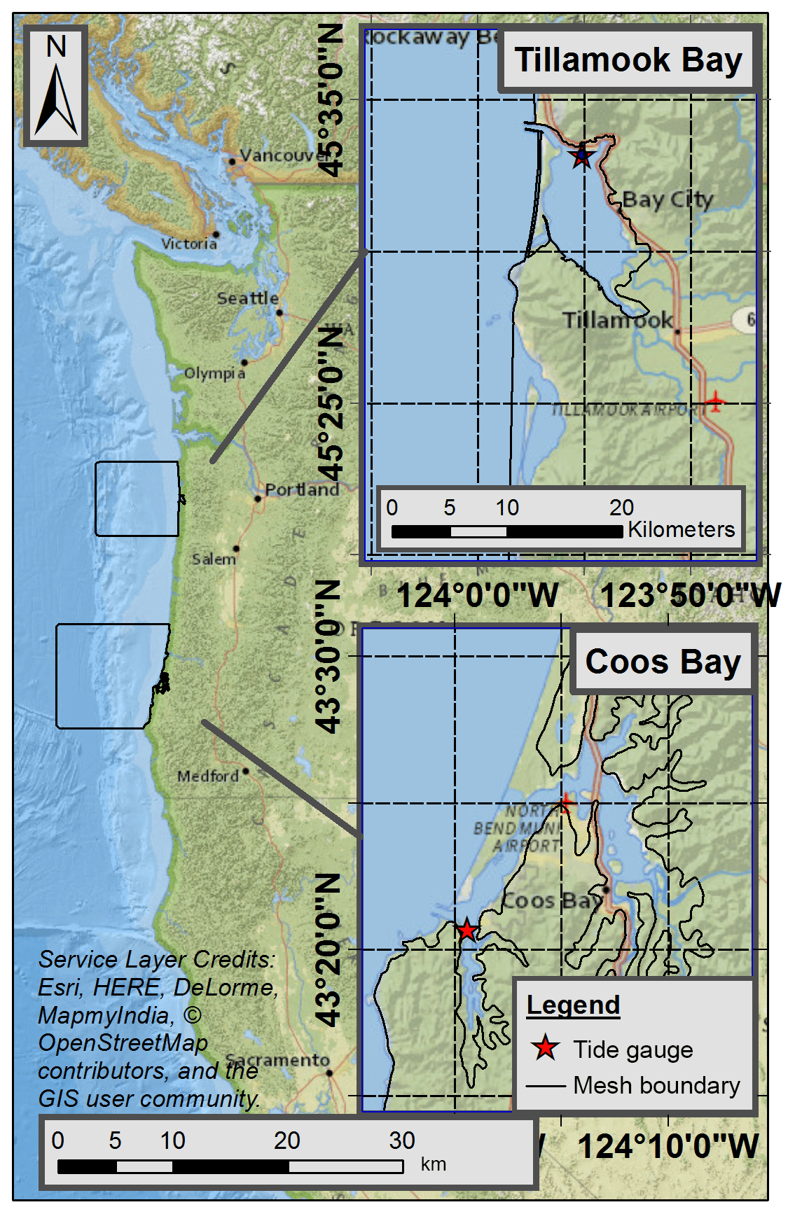
Figure 1Overview map (left) and detailed views (inset boxes) of Tillamook and Coos bays on the US Pacific Northwest coastline. Both insets are at the same scale (shown on Tillamook Bay inset). The tide gauge locations are shown as red stars and the mesh boundary is shown as a dark line in both the overview and detailed view boxes.
Table 1Coos and Tillamook estuarine characteristics (after Engle et al., 2007). Wind characteristics are at tide gauge locations. Wave characteristics are offshore at buoys 46002 and 46005. Streamflow values are from this study's hydrological analysis.
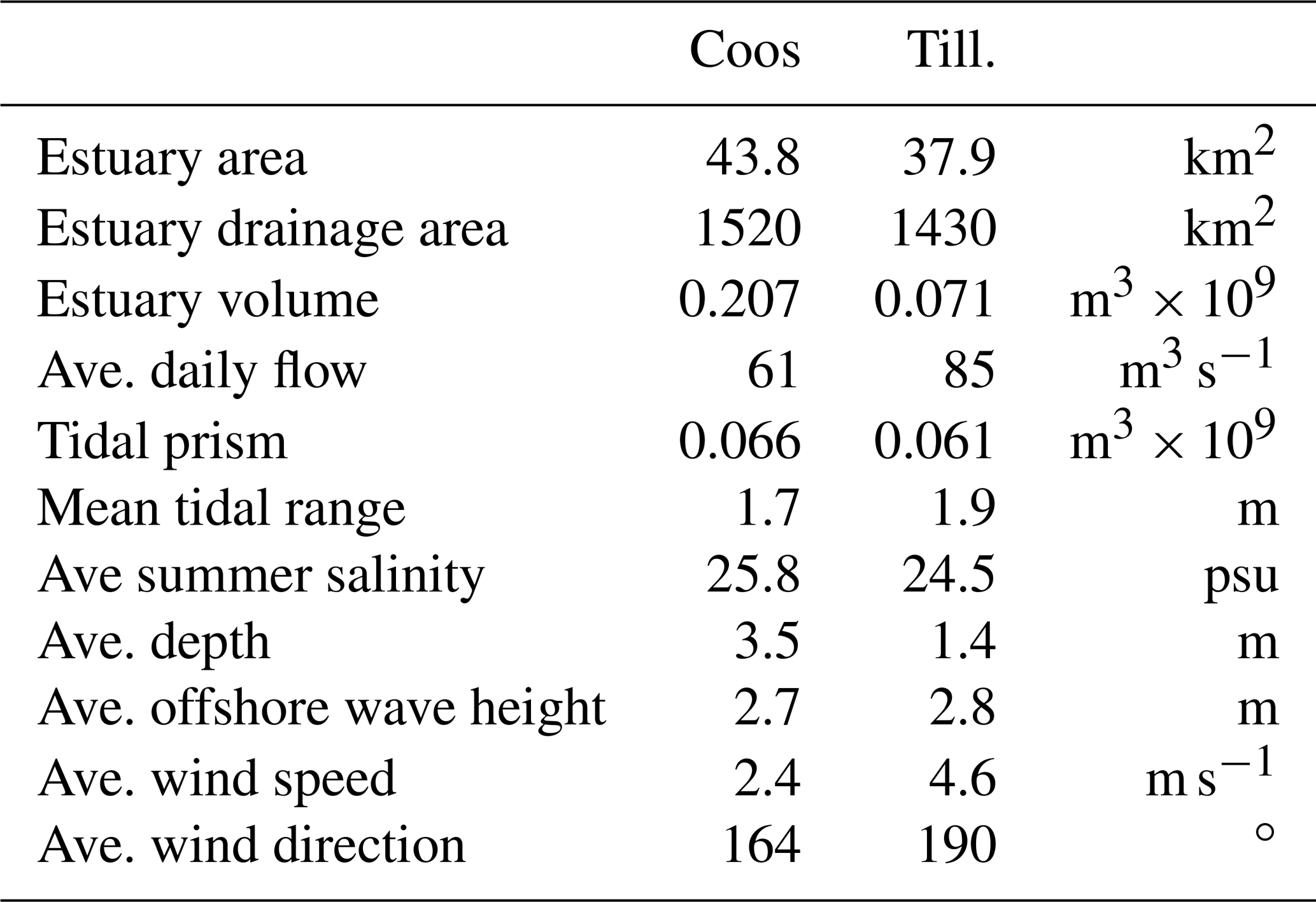
This study focuses on two US PNW estuaries, Coos and Tillamook bays (Fig. 1). These estuaries were selected for two reasons. First, each has an active watershed–estuary organization (Coos Watershed Association and Tillamook Estuaries Partnership), which allowed for data sharing and project collaboration. Secondly, the estuaries have similar forcing profiles (Table 1), which maintains some degree of comparability between the two locations. However, the estuaries have very different physical characteristics, which allows some exploration into the importance of local bay configuration.
In terms of physical layout, Coos has a unique hook shape while Tillamook has a more classical bay form with an enclosing sand spit defining the western edge (Fig. 1). Both estuaries have a jettied inlet and a channel maintained by the U.S. Army Corps of Engineers. Tillamook's entrance is maintained at 5.5 m deep and 60 m wide while Coos has a significantly larger deep-draft channel at 18 m deep and 210 m wide. Coos has a larger average depth and surface area, resulting in a greater estuary volume than Tillamook by around 130 million m3. Coos is also narrower with a deep channel along the majority of its length. Tillamook, however, has a channel only near the entrance with the bulk of its area being defined by broad shallow tidal flats.
In terms of forcing, the estuaries are quite similar, although Tillamook experiences slightly higher environmental forcing. Tillamook's tidal range is approximately 20 cm larger than Coos and mean wave, wind, and streamflow forcing are all modestly more intensive.
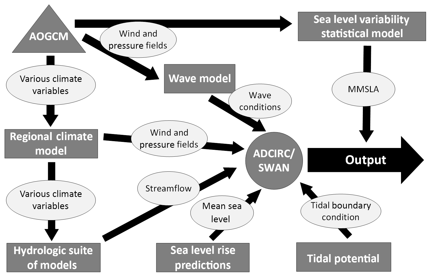
Figure 2Overview of the general modeling framework. The dark gray triangle labeled AOGCM in the top left corner is the “parent” model. Dark gray rectangles represent sub-models. Light gray ovals represent variables that are passed between modeling components.
This study utilizes a suite of models and data sources to determine the hydrodynamic response of the study sites to climatic forcing. The overall workflow is that an atmosphere–ocean global climate model (AOGCM) serves as the “parent” model providing forcing to a suite of “child” models. These in turn provide the forcing to a hydrodynamic model focused on the estuaries themselves. This modeling framework is conceptually illustrated in Fig. 2. In terms of final-stage output, this modeling chain produces continuous time series of WLs (and other variables) at chosen output points. Provided that a sufficiently long-term simulation is carried out, this spatially explicit information allows for the development of flooding inundation maps at a variety of RIs. The following sections describe each component of the model framework identified in Fig. 2.
As is common in climate change impact studies, this study uses paired simulations with hindcast and forecast boundary conditions. Two simulations were carried out; one for the period 1979–1999 (historic) and the other for the period 2041–2070 (future). The historic period is forced with model output rather than direct observations to control for biases in the AOGCM and modeling framework.
3.1 Climate model
This study uses model data from the North American Regional Climate Change Assessment Program (NARCCAP) (Mearns et al., 2009). NARCCAP provides an ensemble of AOGCMs paired with higher-resolution regional climate models (RCMs) focused on the North American continent. The project's future runs are forced by the Special Report on Emissions Scenarios (SRES) A2 emissions scenario, which represents one of the higher-emissions, anthropologically controlled climate scenarios for the IPCC Fourth Assessment Report (Nakicenovic et al., 2000). This scenario was chosen (by NARCCAP) as a conservative but plausible climate trajectory that is in line with current emissions and population patterns. There are other downscaled climate products available (e.g., MACA; Abatzoglou, 2013) that are based on more current IPCC Fifth Assessment scenarios; however, NARCCAP was the only climate product, at the start of this project, that provided the necessary offshore coverage with the higher-resolution RCM. Most other products were masked (and still are) so that data were only available on land surfaces while this project required information across the ocean as well. Spatial resolution for models within NARCCAP is 50 km for RCM variables and ranges from 1 to 4∘ latitude–longitude for the AOGCM models.
While the usage of NARCCAP data forces this project's reliance on an older climate scenario, this does not mean that results are out of alignment with current climate projections. Rather, the A2 SRES scenario is well within the variability of the new scenarios' framework of the IPCC Fifth Assessment. A direct comparison of IPCC Fourth and Fifth Assessment climate scenarios is impossible due to a conceptual change in how scenarios are handled (Nakicenovic et al., 2014; O'Neill et al., 2014). However, work by Van Vuuren and Carter (2014) has shown that the A2 SRES scenario approximately maps to the Representative Concentration Pathway (RCP) 8.5 and shared socio-economic pathway (SSP) 3 scenario. Since the publication of the IPCC Fourth Assessment, baseline emissions have been within the range presented within the SRES scenarios (IPCC, 2007) with emissions tracking closer to the higher range of scenarios (Allison et al., 2009). This supports the usage of the A2 scenario for near-term projections.
From the model pairings available in NARCCAP, the Community Climate System Model–Canadian Regional Climate Model (CCSM–CRCM) combination was chosen as providing the best agreement with local in situ meteorological data. The AOGCM component of this pairing was used for datasets requiring larger spatial coverage while the more finely resolved (both temporally and spatially) RCM was used for nearshore or terrestrial sub-models. When using RCM data, it was found that atmospheric parameters were biased so a univariate statistical bias correction (quantile mapping; Déqué, 2007) was performed. The “target” dataset used for the bias correction was the North American Regional Reanalysis (NARR) (Mesinger et al., 2006) dataset interpolated to the location of the CRCM grid nodes. AOGCM data were also found to be biased but were not bias corrected as there is no target dataset that spans the full global climate model extent. Instead this bias correction was handled within the relevant sub-model.
3.2 Wave model
A basin-scale WAVEWATCH III v3.14 (WW3) (Tolman, 2009) simulation was performed in order to characterize wave climate and provide offshore wave boundary conditions for the two hydrodynamic model domains. WW3 has seen significant success in the US PNW for reproducing wave conditions (e.g., Garcia-Medina et al., 2013) and is well suited to application at large scales (Hanson et al., 2009). The model was run with two nested grids based on the operational global and northeast Pacific models of the National Centers for Environmental Prediction (NCEP) with a resolution of 1∘ by 1.25∘ and 0.25∘ by 0.25∘, respectively. The model was configured with default options and the Tolman and Chalikov (1996) source term package.
Wind forcing for the WW3 model was provided by the CCSM global model. Wave model predictions were found to exhibit a significant bias in comparison to observed wave parameters in the study areas. This bias is likely a result of the low-resolution wind fields (Holthuijsen et al., 1996) or the AOGCM's inability to reproduce marine winds (Hemer et al., 2011). The transfer of bias from wind fields to wave model output has been similarly reproduced and discussed in other studies (Feng et al., 2006; Hemer et al., 2011). Sensitivity analysis showed that running the hydrodynamic model with overpredicted wave heights produced unrealistic flooding values and overwhelmed the influence of other signals contributing to extreme WLs. Therefore, a bivariate statistical bias correction technique (Piani and Haerter, 2012) was used that corrects both the marginal distribution of significant wave height (Hs) and peak wave period as well as maintains the correlation structure (Parker and Hill, 2017).
3.3 Hydrological model
Streamflow inputs were developed using a series of weather, snowmelt, and hydrological routing models. Specifically, the MicroMet–SnowModel–HydroFlow suite of spatially distributed models were used (Liston and Elder, 2006a, b; Liston and Mernild, 2012). Readers are directed to the source citations for full details of the models. In summary, this suite distributes relevant meteorological forcing variables, computes the surface energy balance to simulate snowpack evolution and melt, and then uses a simple linear reservoir-routing procedure to route the runoff from rainfall and snowmelt across the landscape to the coastline. This modeling suite allows for both high temporal and spatial resolution of hydrologic processes (for this study, 100 m grid cell size and a 3-hourly time step). Cheng et al. (2015a) successfully applied this modeling suite to the PNW and Beamer et al. (2017) to the US Gulf of Alaska watershed under climate change scenarios.
The models were calibrated and validated using the NARR dataset for meteorological forcing. Only the Tillamook Bay watershed contains active stream gauges. Therefore, the model was calibrated to observed streamflow at the available gauge locations, the Wilson, Trask, and Miami rivers. After calibration, validation against observed streamflow yielded high Nash–Sutcliffe efficiencies (NSEs; Nash and Sutcliffe, 1970) as well as coefficients of determination (R2), indicating that the hydrological model adequately captures the hydrology of the Tillamook watershed. Model calibration parameters derived at the Tillamook basin were then used for the Coos Bay basin. Both watersheds are similar hydrologically, defined by high winter flows driven by rainfall events and low summer baseflows during the dry season. Therefore, it is expected that similar calibration coefficients should apply to both study sites.
After calibration and validation of the hydrologic models with observed data, simulations were then performed using CRCM input. For consistency with other aspects of the model framework, CRCM variables were all bias corrected using quantile mapping (Déqué, 2007), with the NARR dataset as the target. A full description of the utilized bias correction procedure, both the bivariate method utilized for wave modeling and the univariate method used for other variables, is beyond the scope of this paper. Instead, the reader is directed to Parker and Hill (2017) for a more detailed description.
The gridded hydrologic model produces a daily time series of streamflow at every coastal pour point along the coastline. However, the majority of these locations have small contributing areas and thus produce very low flow values. Only the pour points with large contributing areas (watersheds) and streamflow rates were selected for inclusion in the hydrodynamic model. For Tillamook, data from the mouths of four rivers were included (the Kilchis, Wilson, Miami, and Trask), which were found to capture 95 % of the basin annual streamflow. For Coos, seven points were chosen for inclusion representing 90 % of the basin annual streamflow. The streamflow from these points was aggregated into three inputs into the hydrodynamic model at the location of the Coos River, Palouse Slough, and Noble Creek (Fig. 3).
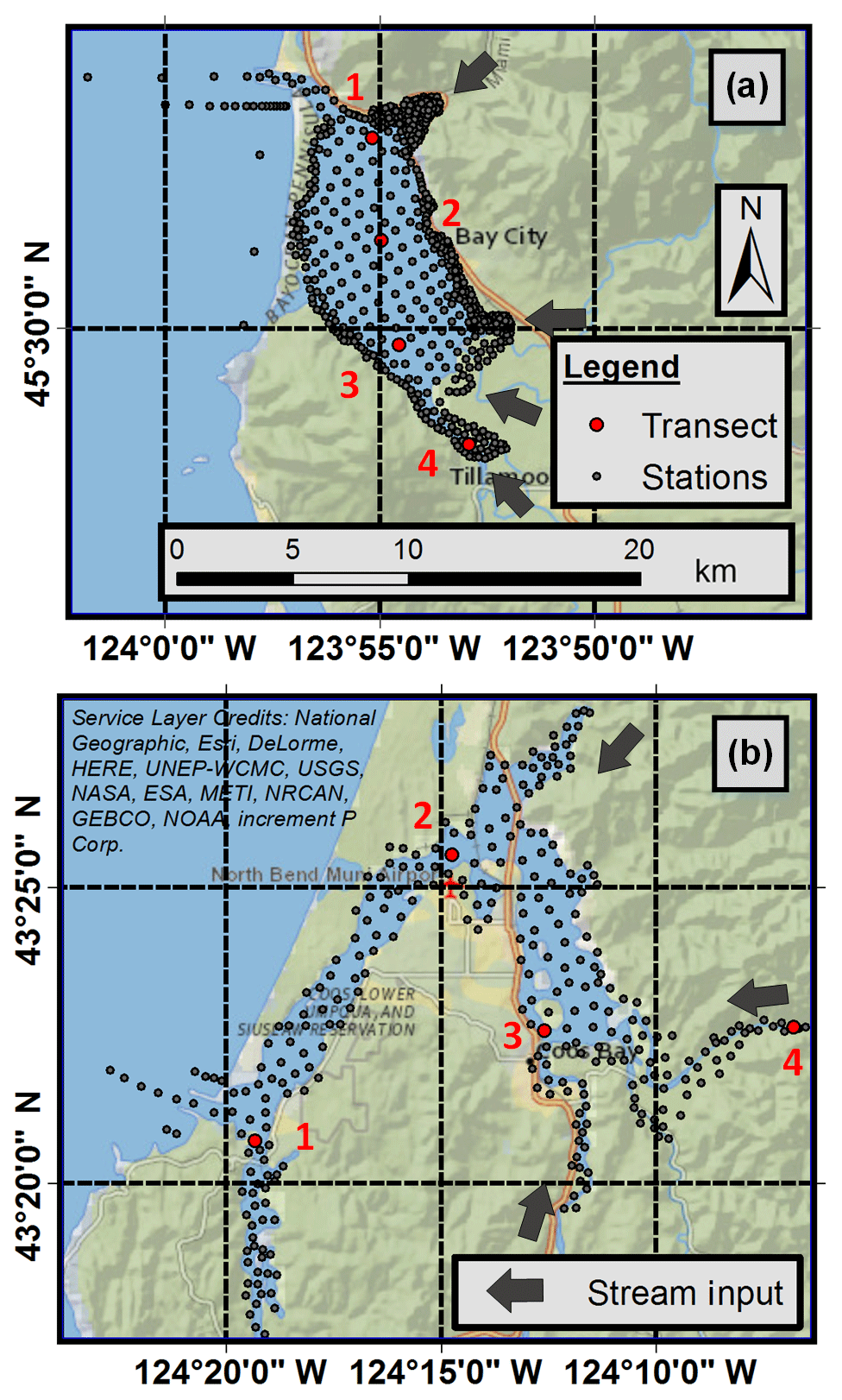
Figure 3Station output locations at the Tillamook and Coos bay study sites, (a) and (b), respectively. Gray arrows show hydrologic inputs into the model domain. Red points and numbers represent transect station locations (see Sect. 6.1). Both figures are at the same scale (a).
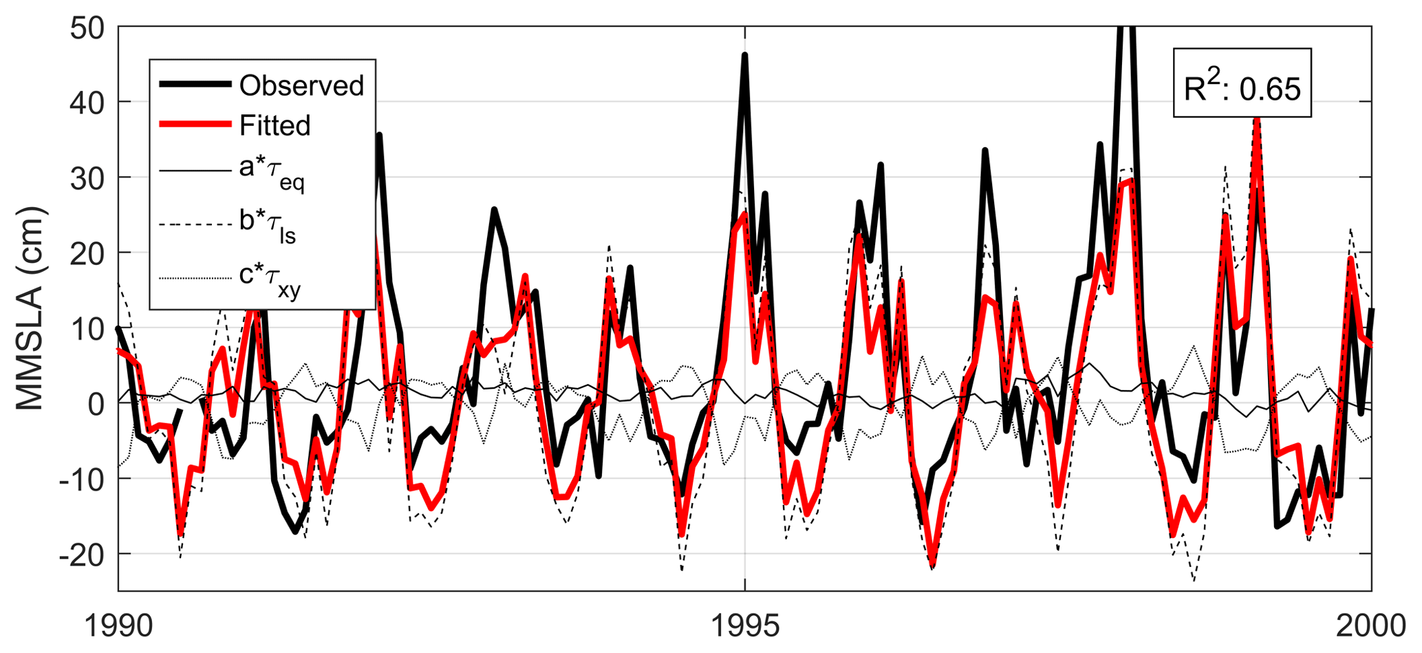
Figure 4MMSLA regression for the Tillamook study site in the style of Thompson et al. (2014). Fitted contributions to MMSLA from predictor variables τeq, τls, and τxy are shown as thin black lines (full, dotted, and dashed, respectively). The bold black line is the observed MMSLA signal while the bold red line is the total fitted MMSLA signal.
3.4 Monthly anomaly model
An important component of measured WLs along the west coast of the US comes from monthly mean sea level anomalies (MMSLAs). These low-frequency variations in WLs are caused by a wide variety of forcings ranging from local wind stress to large-scale climate patterns (such as El Niño) (Allan et al., 2002; Chelton and Davis, 1982). A comprehensive understanding of MMSLAs remains complex, as they integrate a large number of simultaneous processes operating over a wide range of spatial and temporal scales. However, there have been many attempts to model the leading-order terms found in MMSLA signals. This study follows the work of Thompson et al. (2014), who used statistical regression and a subset of wind stress metrics to successfully reproduce the bulk of MMSLA variability across the west coast. The utilized regression is given by
where η is monthly mean sea level, η0 is the regression y-intercept term, τeq is the equatorial wind stress, τls is the local alongshore wind stress, τxy is the wind stress curl, ϵ is the residual error, and (a, b, c) are regression coefficients. The reader is directed to the original source publication for additional information regarding the specifics of the wind stress coefficients as well as their scientific basis.
Figure 4 shows the result of this regression for the Tillamook study site (Coos is not shown). While this formulation does not capture all variability in MMSLA (R2≈0.6), it does qualitatively capture the MMSLA signal and is based entirely on variables that are readily available from the NARCCAP dataset. Furthermore, a statistical approach is attractive since directly modeling coastal MMSLAs would be very computationally expensive. The regression approach is found to somewhat underestimate extreme values of MMSLA, which may introduce a low bias in calculated extreme total water levels. This bias should be similar for both the historic and future periods, so its effect on changes between those periods should be minimal. MMSLAs are added to the hydrodynamic model time series as a post-processing step (see Fig. 2). Not including MMSLA within the hydrodynamic model may exclude some potential nonlinear interactions between MMSLAs, WLs, and other forcings.
3.5 Sea level rise
SLR was included in the modeling framework as a change to mean sea level (MSL) within the hydrodynamic model. Projections were taken from the National Resource Council (NRC) report (NRC, 2012), which developed local estimates for SLR along the US Pacific coast. These estimates include contributions from steric/dynamic ocean modifications, glaciers and ice caps, sea level fingerprint effects, and vertical land motion (e.g., isostatic adjustments). In calculating local SLR estimates, the NRC used a combination of IPCC Fourth Assessment projections (midrange scenario) and an extrapolation methodology for the cryosphere components. This produced values larger than either the IPCC Fourth or Fifth Assessments but still below some estimates for mean 2100 global SLR (Vermeer and Rahmstorf, 2009).
SLR data were taken from the nearest reported location to Coos and Tillamook Bay, Newport, Oregon, which is situated approximately between the two study sites. The NRC report provides projection values (and ranges) for 2030, 2050, and 2100. A cubic spline was fitted to these values to allow a smooth interpolation to intermediate years. Multi-decade model runs of the hydrodynamic model were broken into smaller 3-month periods and MSL was updated accordingly for each of these simulation blocks. This allowed for changes in MSL in a step-wise but nearly continuous fashion.
3.6 Local hydrodynamic/wave model
The coupled ADCIRC–SWAN (ADCSWAN) model (Dietrich et al., 2011b) was used for this study. ADCSWAN is highly configurable in terms of implemented physics and readers are directed to the source publication and model manuals for a full description of options and parameters. ADCIRC (Luettich and Westerink, 1992) solves the hydrodynamic portion of this pairing through the shallow-water equations. ADCIRC uses an unstructured horizontal grid, which allows for finer spatial resolution in regions of complex bathymetry. Bathymetry for the model grid was developed through blending Oregon Department of Geology and Mineral Industries (DOGAMI) lidar (DOGAMI, 2009) and a variety of National Oceanic and Atmospheric Administration DEMs (NOAA, 2018). Wetting and drying were enabled due to the significant intertidal areas present in both bays. Nonlinear bottom friction was used with a spatially variable friction factor set based on general land use classes (Dietrich et al., 2011a; Homer et al., 2015).
ADCIRC was run, for this study, in the 2-D depth-integrated (2DDI) mode. Previous research has shown that storm surge and tidal signals can be accurately resolved by 2-D barotropic models. Specifically, Resio and Westerink (2008) point out that 3-D effects are readily absorbed by model calibration coefficients. Additionally, a sensitivity study by Weaver and Luettich (2010) found that differences in predicted WLs between 3-D and 2-D models were on the order of 5 % over most of the domain. These modest differences suggest that a 2-D model can be an effective and efficient choice for studies of this type.
SWAN is a third-generation spectral model that solves the spectral action balance equation to compute the spectral evolution of wind waves. The unstructured format of SWAN (Zijlema, 2010) was utilized to allow tight coupling (on the same grid) with ADCIRC. SWAN was run in a nonstationary mode with offshore forcing provided by a temporally varying JONSWAP spectrum fitted to bulk wave parameters.
ADCSWAN was run with atmospheric forcing provided as gridded horizontal wind components and surface pressure, wave forcing using SWAN's nonstationary TPAR parametric spectrum file, hydrologic input as a normal flux into the domain, and tidal forcing at the ocean boundaries. Tidal forcing was defined as the eight locally dominant constituents (K1, O1, P1, Q1, M2, S2, N2, and K2) with location-dependent amplitudes and phases defined by the ENPAC tidal database (Mark et al., 2004) and the simulation time-dependent nodal factor and equilibrium argument defined by the T_tide harmonic analysis package (Pawlowicz et al., 2002). The ADCSWAN model was first validated at each study site using a tidal simulation compared against NOAA tide gauge predictions. Using a 1-month simulation, both the Tillamook and Coos grids were found to have R2 values greater than 0.97. The Tillamook model was additionally validated against the largest storm of record (the Great Coastal Gale of 2007; Crout et al. 2008) with good agreements to extreme WLs (Cheng et al., 2015b).
This study primarily considers extremes, which will be quantified in terms of RI events, since engineering design and community planning often rely on this concept. The traditional definition of an RI is built on an assumption of stationarity, or time invariance. This assumption makes the definition of a RI simultaneously the inverse of the probability that an event of a given magnitude will be exceeded in a given year and the expected recurrence period of that event. This definition breaks down under nonstationary conditions, which can be experienced due to climate change and/or SLR. Reconciling a nonstationary environment with traditional design methods based on stationary assumptions is an ongoing challenge. Proposed alternatives include effective design value (Katz et al., 2002), expected waiting time (Olsen et al., 1998; Salas and Obeysekera, 2014), expected number of events (Parey et al., 2007, 2010), design exceedance probability, and design life level (Rootzén, 2013). Each of these definitions represents a unique projection of the stationary case for nonstationary conditions. Problematically, the chosen metric can result in significantly different calculated RIs while most users simply interpret the result as comparable to the stationary case. This highlights the importance of rigorously defining utilized nonstationary RI formulation as well as considering if the utilized metric fits design conceptions.
Nonstationary extreme value analysis has recently seen a wide range of applications to coastal problems (Corbella and Stretch, 2012; Katz, 2013; Wahl and Chambers, 2016; Wahl et al., 2015). Nonstationarity is generally incorporated within the statistical model by using time-dependent parameters as either a linear or exponential function (Cheng et al., 2014; Ruggiero et al., 2010), a cyclical trigonometric function (Méndez et al., 2008; Mínguez et al., 2010), or a more complicated function of covariates (Méndez et al., 2007; Weisse et al., 2014). Even for stationary extreme value analysis there is a range of commonly used statistical models with a corresponding uncertainty as a result of the chosen methodology (Wahl et al., 2017). Across the wide variety of applications of nonstationary extreme value analysis, no consensus definition of nonstationary RIs or a best-practice methodology has emerged.
This study approaches nonstationary RIs using the effective design value interpretation (Katz et al., 2002). This defines a temporally varying RI (termed an effective RI, or design value, by Katz et al., 2002) which holds the probability of occurrence for an event constant through time. This preserves an intuitive definition of RIs as well as how nonstationarity impacts extremes. Effective RIs add an additional dimension of time (in comparison to standard RIs) so are commonly presented as a family of curves with time on the x axis, event magnitude on the y axis, and each curve representing a recurrence interval (e.g., 2-year event). Additionally, this means that the specification of an effective RI requires both a recurrence interval and a time of interest (e.g., a 100-year event for 2050).
The effective RI definition of nonstationarity is chosen for this study due to the unique format of the results. WL data are output from the modeling framework in reference to MSL. Therefore, the WL time series does not show any discontinuity or trend from changing sea level, a signal that would only be visible if viewing WLs relative to a nontidal datum. This results in an approximate stationarity, as a function of datum, and makes it possible to separate the calculation of RIs from the nonstationarity of the time series. In this context, calculating effective RIs reduces to calculating the stationary RIs and then adding SLR (the assumed nonstationary component) to these estimates.
The benefit to this approach is that it avoids the complications of fitting a nonstationary generalized extreme value (GEV) distribution and the corresponding loss of degrees of freedom from estimating the nonstationary trend from the data. Furthermore, most nonstationary GEV analyses are forced to use a priori simplistic functions due to limited degrees of freedom. This approach allows a more complicated trend that follows experienced SLR (approximately cubic for this study). The negative of the approach is the assumption/simplification that the resulting MSL time series is stationary. While this is a common statistical assumption, it does have consequences for the results and is discussed further in Sect. 6.4.3.
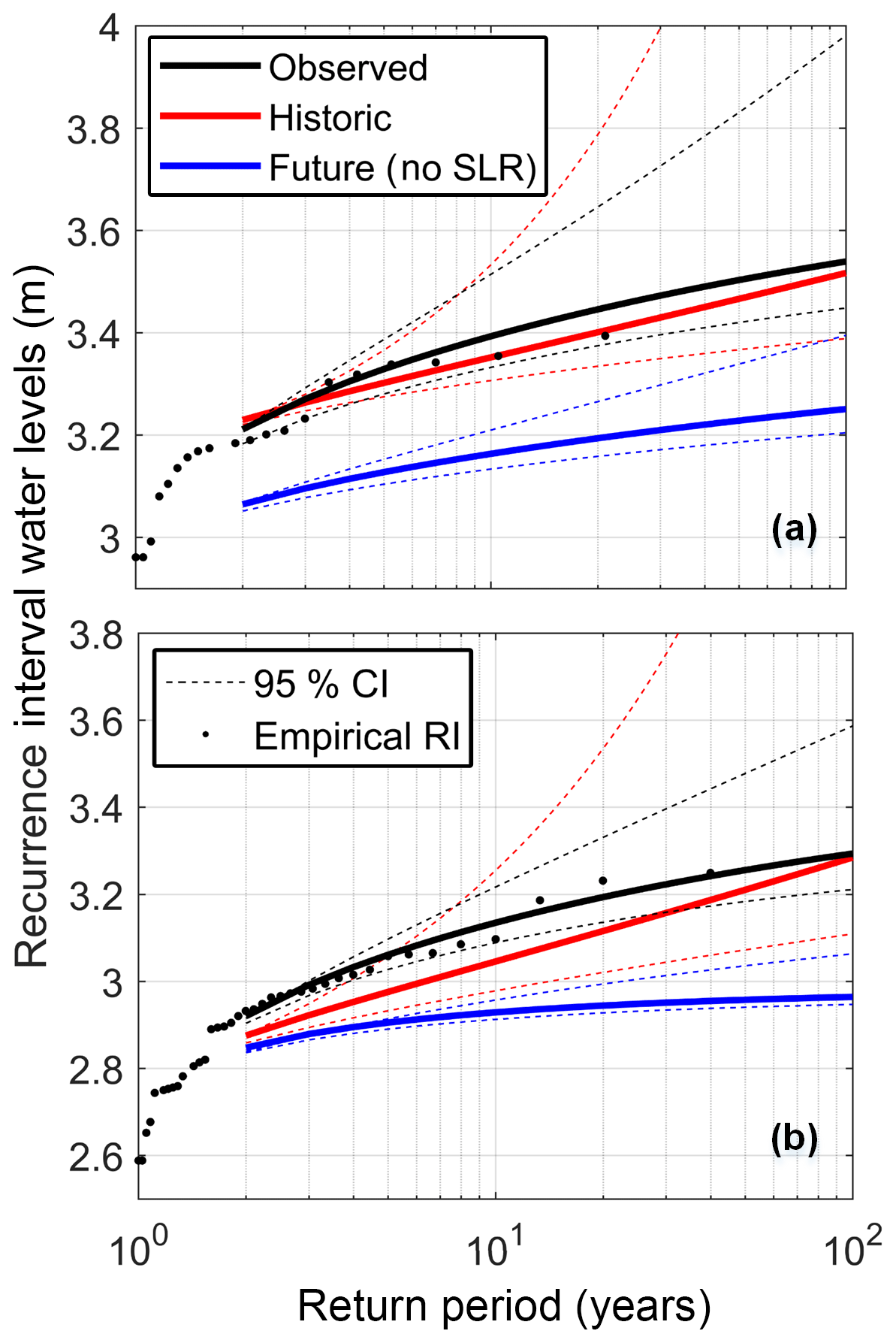
Figure 5RIs for the Tillamook and Coos bay tide gauges, (a) and (b), respectively. WLs are in the NAVD88 datum. Confidence intervals are only for statistical uncertainty in the GEV model and are calculated using a likelihood-based method (plotted as dotted lines). SLR has not been included for future RI curves.
Model output was saved at a subset of model nodes (stations) in order to keep output files manageable in size. Output stations were spaced evenly across the bay in order to capture spatial variability (Fig. 3). While ADCSWAN has the ability to write out numerous variables (including wave heights, periods, etc.), the focus of this study is on WLs so discussion here will be limited to that variable. The model was run in 3-month-long segments with a 2-week overlap to avoid discontinuities in dynamic processes. Smaller segments were necessary for integrating SLR as well as for model stability reasons. Output data from these segments were then recombined into continuous time series at each station.
Analysis was performed for both the historic and future periods. With an identical configuration (for all modeling components) to the historic period simulation, the only free variable is the AOGCM forcing under climate change. Therefore, a comparison shows how extreme events can be expected to change (in a relative manner) over time.
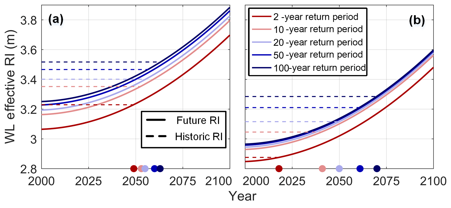
Figure 6Tillamook (a) and Coos bay (b) effective RI WLs for the historic (dashed line) and future (solid line) periods. Shorter return periods are represented as warm colors while longer return periods are plotted as cool colors. The location of intersection between the historic and future effective RI curves is plotted on the x axis as a dot with color corresponding to return period. The x- and y-axis scaling is the same in each subplot.
5.1 Recurrence intervals (tide gauge locations)
RIs were calculated using a GEV distribution fitted to annual block maxima events. Figure 5 shows this analysis for observed, modeled historic, and modeled future (without SLR included) time series at the Coos and Tillamook bay tide gauge locations (Fig. 1). The calculated historic period RI curve for Tillamook (Fig. 5a) exhibits good agreement with observations with a maximum offset of around 4 cm. The agreement is less favorable for Coos Bay (Fig. 5b), with a maximum offset of around 9 cm. For both locations, the largest difference between observed and modeled RIs is for medium (approximately 10 years) RI events. This is because both modeled RI curves exhibit a different curvature than the observed RI curves. A possible source in the low bias for modeled RIs may be the low bias observed in the MMSLA regression model.
It is important to note that Fig. 5 includes future RI values plotted with SLR not included. This plot shows a comparison of the future return intervals (assumed stationary with SLR removed) to the stationary historic period return intervals. Since nonstationary and stationary return intervals are not generally equivalent, this provides a manner of comparison. Using the effective design value interpretation, this can be thought of as future RIs but with the chosen design year being 2000. Practically this shows future RIs as a function of only changing forcing (no SLR). Both plots show the future RI curve as exhibiting smaller WLs than the historic RI curve, hinting at a reduction in extreme WL forcing into the future.
Figure 5 presents results in a classic RI curve format but they can additionally be viewed as effective RIs (as described in Sect. 4). Effective RIs were developed by calculating stationary RIs from the WL time series (relative to MSL) and then adding SLR (Fig. 6). Figure 6 contains both the future and historic effective RIs on the same plot to visualize how RIs change upon entering a nonstationary climate regime. Based off model assumptions, historic effective RIs are flat lines through time (as they include no nonstationary component). Figure 6 reiterates the same RI behavior as above with historic RIs being higher than future RIs for the current period (year 2000). Moving forward in time, this plot shows that SLR eventually overtakes this effect to result in a higher future flood. The point of overtake (where nonstationary RIs begin to predict a larger flood) is plotted in Fig. 6 as colored dots on the x axis. This intersection is significantly earlier for short RIs (within 20 years for a 2-year event) than for longer-RI events (over 60 years for a 100-year event). This result is shown for both estuaries but with Tillamook Bay having less spread in overtake time than Coos Bay.
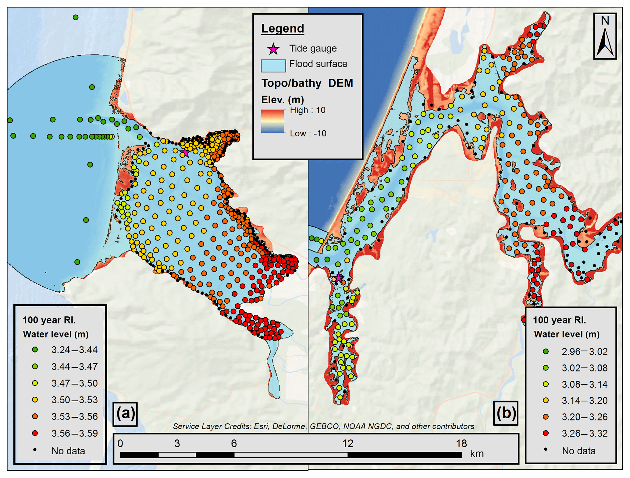
Figure 7Historic period 100-year flood surface results for Tillamook (a) and Coos (b) bays. Individual stations are plotted with color scale indicating the modeled 100-year-RI WL magnitude for the historic period. Note that the color scale is different between the two study sites. The calculated flood inundation surface is plotted as a blue transparent region.
5.2 Recurrence intervals (spatial variability)
Section 5.1 discusses RIs at a single location (the tide gauge), but a key feature of this study's methodology is the ability to explore spatial variability in RIs across the study sites. Figure 7 demonstrates this by plotting the 100-year-RI WL calculated for the historic period at each output station. Analysis was limited to stations that were wet over 75 % of the record length. This was implemented to limit uncertainty in GEV analysis due to insufficient record lengths at only periodically wet stations.
It is apparent in Fig. 7 that there is a significant gradient in extreme WLs across both study site estuaries. For Tillamook, WLs differ by approximately 25 cm and for Coos by around 35 cm. The gradient in WLs is oriented such that the minimum WL is located near the estuary entrance with extreme WL height increasing with further distance into the estuary. Of particular interest, this trend is the same for both study sites, suggesting that this pattern may be more generally applicable. While Fig. 7 only plots the 100-year event, this extreme WL differential is maintained across other RI periods.
The spatially variable WLs produced from this analysis provide the necessary information for building flood maps. This was accomplished by fitting a smooth surface to the scattered stations using spatial spline interpolation (ESRI, 2016). The 100-year-RI WL surface was then intersected with the estuary DEM with all locations below the extreme WL surface defined as “flooded”. This methodology makes the assumption of extrapolation at the edge of the surface where station output was not available. The calculated flood surface is shown in Fig. 7 as a light blue surface. Comparison of this surface to the US Federal Emergency Management Agency (FEMA) 100-year floodplain for Coos Bay (FEMA, 2014) (not shown) revealed that the produced flood inundation zones are different, but not greatly so. This is likely more attributable to Coos Bay's steep topography than to similarities in produced hazard levels. Planform flood area is highly influenced by terrain gradients and large variabilities in predicted hazards can manifest as only small changes to flood zone for steep shorelines. FEMA only produces flood map products, so a more quantitative comparison of extreme water levels was not possible.
5.3 Changes to recurrence interval spatial structure
Section 5.2 details the importance of considering spatial variability in extreme WLs but only considers the historic scenario. An important question remains as to how this spatial variability can be expected to change moving into the future. This is especially important as, while individual flooding estimates might be biased (for example by the inability of the MMSLA regression to produce extremes or by bias in the forcing AOGCMs), these biases should cancel when calculating change from the historic to future scenarios. Figure 8 explores this analysis by plotting the difference between future effective 100-year-RI WLs (calculated for the year 2050) and historic 100-year-RI WLs.
As a primer, if the RI difference plot (Fig. 8) showed no spatial variability, then the same pattern seen in Fig. 7 would be replicated in the future, with only a vertical offset. This would be an important result signifying that the spatial pattern of current extreme flooding events will remain unchanged into the future with only an estuary-wide SLR adjustment being required to update hazard assessments. Instead, Fig. 8 shows a spatial pattern that is qualitatively similar to that seen in the historic RI plots. Specifically, results show that the change in WLs increases with further distance into the estuary, a result that signals an increase in the spatial gradient of RIs as the study sites move into the future. Looking at other RI event periods (not shown), results show a gradual decrease in changes to spatial variability from around 10 to 20 cm for the 100-year-RI event to approximately no change for the 2-year-RI event. Note that the choice to plot effective return intervals for the year 2050 is arbitrary and does not affect the spatial pattern of differences (the critical information in this plot). A different design year would only change the overall magnitude, not the inter-point variability/pattern. Also included in Fig. 8 is the 100-year recurrence interval flood zone for the historic period and for the effective RI design year of 2100.
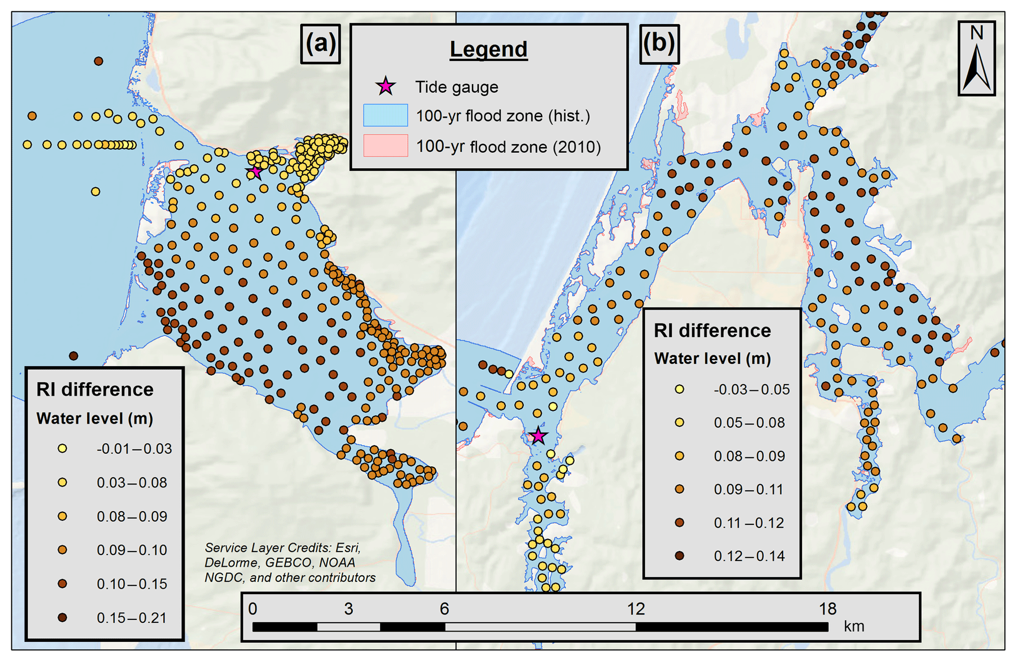
Figure 8Changes to 100-year RIs plotted at output stations. Changes are calculated as the future effective RI WL (at year 2050, 0.172 m of SLR) minus the historic RI WL. The blue surface is the calculated historic 100-year floodplain while the red surface is the future 100-year flood surface calculated for the year 2100.
6.1 Drivers of extreme water levels
The spatial variability of extreme WLs shown in Fig. 7 motivates further investigation into what physical processes are controlling WLs in different regions of the study areas. This was investigated by carrying out a series of 17 d simulations bracketing the largest observed event at each study site and for each time period. Each simulation in the series was performed with an individual forcing component turned off (e.g., wind, streamflow). The WL contribution from each forcing was then calculated by subtracting the simulation with the forcing of interest turned off from a simulation with full forcing. Therefore, each component can be conceptually thought of as quantifying the contribution of each forcing of interest to the total maximum WL. Figure 9 summarizes the breakdown of contributions at several locations (moving up the estuary) at each study site, and for both historic and future periods. Components are plotted at the time of maximum WL occurrence.
The results show that, for the simulated events, pressure and MMSLAs are the largest components of nontidal residual (tides are not shown in Fig. 9). As MMSLAs are a source of uncertainty in this study's modeling framework, this motivates a need for further improvement of MMSLA estimates. This could potentially be accomplished through either improved statistical methods or a computationally tractable physical modeling approach. Streamflow and offshore wave forcing were found to be an order of magnitude less important than pressure and MMSLA. This is especially true for the two events at the Tillamook study site (Fig. 9c, d) where streamflow and wave forcing were found to be of negligible importance to extreme event WLs. The wind contribution was found to be variable across stations and events. This is expected as wind setup is highly dependent on the estuary geometry and the wind direction of the specific event.
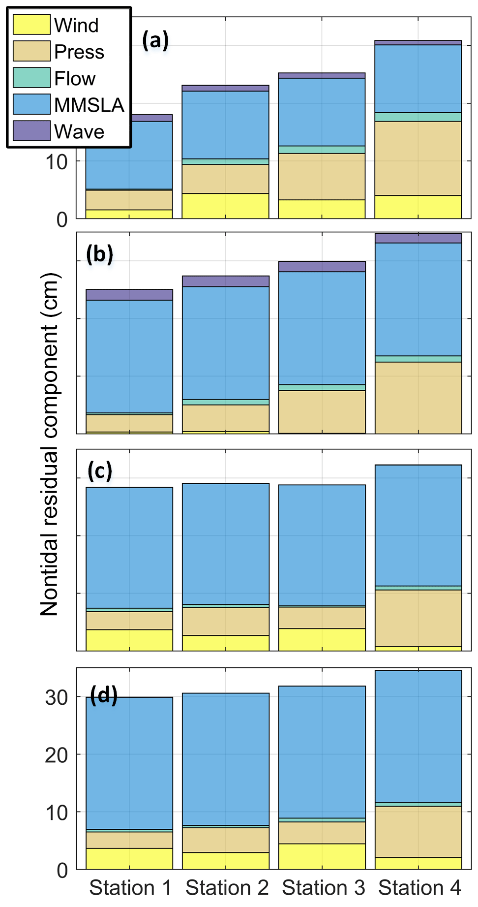
Figure 9WL contributions from various forcings during the largest simulated WL event. Stations transition from the tide gauge (station 1) to the far river outlet of the estuary (see Fig. 3 for station locations). Panels (a) and (b) show the Coos historic and future periods. Panels (c) and (d) show the Tillamook historic and future periods. All panels have the same y-axis scaling.
However, this analysis is only for the maximum annual event and other events likely have different compositions in terms of forcing contributions. Further investigation shows that, for both study sites and both climatological periods, extreme event magnitude is not correlated with any individual forcing (p value > 0.05 when calculating correlation between WL magnitude and forcing magnitude at annual maximum events). This is reinforced by the fact that many annual maximum events are found to occur during below average nontidal forcing conditions (e.g., below average wind or waves). This supports the conclusion that extreme WLs in the PNW are generally compound events, driven by the sum of multiple forcing, that are not necessarily extreme themselves. This result is in agreement with other studies of forcing contributions to extreme events in the PNW (Parker, 2019).
The exceptions to this conclusion are tides and MMSLAs, which are found to have a statistically significant correlation with event magnitude. Tides were not plotted in Fig. 9 for scale reasons but were found to be the largest fraction of WLs (an average of 185 cm for Till and 145 cm for Coos). It follows that extreme WLs would most often occur during (or near) a high tide. Therefore, the concurrent timing of tides and nontidal forcing becomes a major control on WL magnitude. This represents a mechanism explaining the predominance of compound events in the PNW, in which extreme WLs are not necessarily associated with extreme forcing. This is also a potential reason for some forcing components showing a negligible influence on extreme WLs (e.g., waves in Fig. 9). While waves have been shown to be important drivers of nontidal residuals in PNW estuaries (Cheng et al., 2015b; Olabarrieta et al., 2011), tidal modulation means extreme WLs do not necessarily occur during maximum wave energy events.
The resulting evidence of complexity in compound events for the study site confirms that a comprehensive analysis of extreme WLs in the PNW likely requires an approach similar to that taken here. Event-based approaches would likely be ineffective as storms or extreme forcings are not necessarily correlated with max annual events. Additionally, the common methodology of simply adding the largest nontidal residual to a high tide could result in significant overestimations of event magnitude.
6.2 Spatial variability in return intervals
It is common practice to calculate WLs at a convenient location (such as a tide gauge) and then apply this value across the entire study domain. While larger estuaries (e.g., Delaware Bay) may have multiple tide gauges, smaller estuaries typical of the PNW tend to have one or none. A spatially constant assumption represents a major simplification as even tides can produce significant spatial WL variability in semi-enclosed basins (Holleman and Stacey, 2014). Additionally, spatial variability is particularly important for estuaries as they are often regions of low-gradient topography where a modest change in water elevation can correspond to a large change in inundated area. Results (Fig. 7) show variability in WLs for both locations in excess of 25 cm. Furthermore, the smallest WLs are at the estuary mouth where, in the PNW, the tide gauge is generally located. This means that estimating flooding from a tide gauge will result in under-predictions for flooding with errors increasing with upstream distance into the estuary. This result strongly supports the importance of considering spatial variability in WLs within flood hazard assessments.
Between the two study sites, Coos is found to have a larger extreme WL differential (approximately 30 cm from the mouth to the interior bay). This is contrary to the expected result that Tillamook, with its proportionally larger forcing, would have a larger gradient. Streamflow, in particular, was expected to have a significant impact on WLs but was found to have a minimal effect for both study sites. This was particularly true for Tillamook despite its larger average streamflow input. Figure 9 shows that, while the streamflow component does increase moving shoreward for Coos bay, the majority of the WL differential for both sites is driven by pressure. An additional component of the WL gradient is from tidal forcing, which produces around a 10 cm differential between the estuary mouth and the inner bay for both locations.
Results show that spatial variability is predicted to change into the future. However, this result is primarily shown for longer-RI events, with shorter-RI events not showing any change in spatial variability for the future scenario. Shorter-RI period events are better constrained statistically than longer-RI period events so it is possible that some proportion of the predicted spatial variability is a function of GEV analysis on a temporally limited record. A modeled record longer than the period used here (20 years for historic, 30 years for future) could help to illuminate if this conclusion is a physical result.
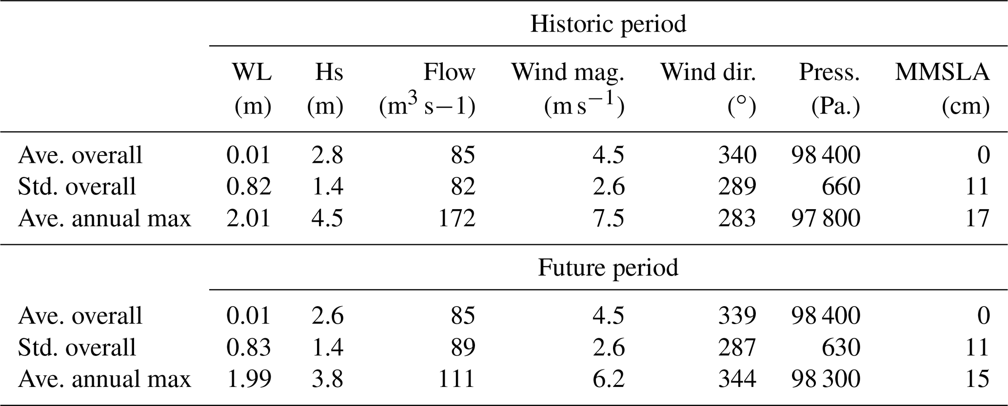
Table 2Comparison of forcing for Tillamook Bay under the historic and future climatological periods. “Ave. Overall” is a full time series average while “Ave. Annual Max” is an average of forcing during observed annual WL maximum events.
6.3 Changing extreme events
With analysis suggesting RIs evolve through time, a natural next question is how climate change is modifying the estuarine system. To help illustrate this, Table 2 shows a comparison of forcing statistics under the historic and future climatological periods for Tillamook. Results show a decrease in most forcing variables, both as an overall average and for average forcing during extreme events. This result is similarly seen for Coos Bay (not shown). This suggests that the decrease in RI shown in Fig. 5 is caused by a broadscale reduction of forcing on the estuary for the AOGCM scenario considered. Unfortunately, with all modeled forcing shown to be reduced for the future period, it is difficult to conclusively differentiate which drivers are controlling changing RIs. Similarly, as GEV analysis is based on a parametric fit of multiple annual maximum events, it is difficult to characterize the cause of changing RIs without considering the aggregate behavior of all the events to which the GEV is fitted (rather than a single event as shown in Fig. 9).
A further exploration of changing RI was shown through effective RIs (Fig. 6). This result found that the reduction in forcing is eventually overcome by SLR, although with the timing being controlled by the size of the RI event. The idea of an “overtake point” is a simplification based on the assumptions within the statistical model, specifically that of stationarity and nonstationarity (see Sect. 6.4.3). Another way of viewing this result is that SLR represents a single value for change across all RIs. By the year 2050, both 2-year- and 100-year-RI events increase by 17 cm due to SLR. Conversely, the change in RI magnitude from forcing is variable across return periods. From forcing, the change in 2-year RI is only 3 cm while for the 100-year RI it is much larger at 32 cm. This means that shorter-RI events are less buffered by a change in forcing than longer-RI events. The conclusion is the same from this interpretation in that short-RI events will be comparatively more impacted by SLR than longer-RI events.
6.4 Modeling limitations
6.4.1 Excluded processes
In this study bathymetry and topography were held constant through time. Bathymetry is a first-order control on flooding and so an ideal future projection would include morphological evolution of the estuary. This said, morphological projections at climate change scales are extremely uncertain. The combination of high uncertainty and high dependence would leave resulting flood predications dominated by an uncertain morphology projection with all other signals obscured. This study therefore does not consider morphological evolution in order to specifically highlight how changing forcing impacts extreme WLs.
Both estuaries have significant anthropological modifications ranging from coastal infrastructure to dredged channels. Coos in particular has an engineered coastline along the majority of its southern boundary. A key factor in future extreme events is the interaction between human intervention and the estuarine system. For example, estuary WL characteristics under tidal forcing show high sensitivity to anthropological changes (Gallien et al., 2011; Wang et al., 2017) and modifications to land use have been shown, in certain cases, to be of the same order of importance to WLs as SLR (Bilskie et al., 2014). Dredging, for the same reason as morphological evolution, can cause drastic changes to estuarine hydrodynamics. However, similarly to morphological predictions, anthropological controls are highly uncertain and therefore not included in this analysis.
6.4.2 Climate model variability
The results shown in Fig. 5 provide an interesting comparison of modeled and observed extremes. However, the modeled results and observed results are not based on the same forcing time series, but rather one observational and one modeled time series. Since both the Coos and Tillamook modeled RI curves have less curvature than the observed curves, this could be a result of the specific climate model iteration that was used for the simulation. The common solution to this problem is the usage of ensembles of climate models rather than a single AOGCM (Murphy et al., 2004). Unfortunately running ensembles is computationally expensive given the level of complexity included in this study. Conceptually this study makes the compromise of including more physical complexity at the cost of uncertainty quantification. Results from this project should therefore not be viewed as a probabilistic or a “most-likely” result from climate change. Instead, they should be thought of as a single possibility of what could happen and an illustration of the importance of including various processes in a study of this type.
Not including multiple model iterations is also problematic in constraining the current climate's RIs. Results in Sect. 6.1 show the importance of compound events and forcing timing (especially tides) at these study sites. While forcing was bias corrected using a methodology that has been shown to perform well for extreme quantiles (Parker and Hill, 2017), timing of forcing occurring on a high tide or during a high MMSLA is additionally critical. This study examines only one possible combination of forcing timings that may or may not be representative of the overall extreme behavior of the system. This could once again be addressed through usage of ensembles or multiple iterations of the current climate.
While results from this study build a strong case that including dynamic coupling of processes is important for flood estimation, a natural next question is the cost/benefit when viewed under the extreme uncertainty of climate change. As an example, this study shows a change in spatial distribution of extreme water levels of 10–20 cm moving into the future. This is significant in terms of hazard quantification but small in comparison to uncertainty in PNW sea level rise by 2100 (on the scale of over 60 cm: Miller, 2018). It is expected that the need to include this uncertainty will likely often preclude the usage of the coupled dynamics employed by this study. Rather it is hoped that these results can provide an idea of the type of errors being induced by using more simplified modeling frameworks. Furthermore, this study provides a strong motivation for methodologies to combine dynamic modeling with faster simulation times. Recent research at a similar estuary study site in the PNW has shown emulation as a promising method to provide this linkage (Parker et al., 2019).
6.4.3 Assumptions of stationarity
Another important assumption in this study is that of stationarity when SLR is removed. The reality is somewhat more complicated as climate change will result in a forcing-driven nonstationarity in addition to that seen from SLR. Research has additionally shown that SLR can be expected to interact nonlinearly with storm surge, creating another source of nonstationarity over time (Buchanan et al., 2017; Devlin et al., 2017; Wahl, 2017). For our case, each time series segment is statistically stationary (Augmented Dickey–Fuller test, p value < 0.001) but the overall time series (from 2000 to 2070) must be nonstationary. This is because the two segments (historic and future) show distinctly different calculated RI curves (Fig. 5) so WL behavior, as controlled by forcing, must be changing. Simply put, this study analyzes two segments that are not long enough to reveal the longer term nonstationary behavior of the overall time series as controlled by changing forcing. This is not problematic for this study, which compares two snapshots, but a comprehensive analysis would need to resolve the overall nonstationarity from forcing as well as from SLR. This is also a factor in the calculation of the overlap timing from effective RIs (Fig. 6) since the overall nonstationarity from forcing is not included in the analysis. Therefore, the overlap timing results should not be considered an exact calculation but rather a general result.
This paper introduced a process-based modeling framework for analyzing climate change impacts on various controls on estuarine flooding. In particular this study focused on extremes and changes to RI events at two PNW estuaries. This study described the difficulty of using RIs in the context of nonstationarity and showed how “effective RIs” can be an intuitive way of understanding changing flood hazards. Effective RIs showed that predicted changes to forcing result in a decrease in extreme event magnitude moving into the future. This decrease buffers the increase in WLs that comes from SLR. This buffering effect was shown to be smaller for short-RI events than long-RI events, suggesting that increasing extremes will be felt first for low-RI events.
This study used multiple study sites and climatological periods to explore drivers of extreme events. It was found that extreme events for both locations were not controlled by a single forcing but rather by compound events. Tides were shown to be the largest contributor to extreme WLs. The requirement for a high (or near high) tide modulates the contribution from other forcings during extreme WLs. This means that high nontidal residual or storms are not necessarily the source of extremes at the study site. This suggests that both event-based methodologies and the common procedure of adding an uncoupled high tide and high nontidal residual will both result in an incorrect assessment of flooding magnitude.
An additional outcome of this study was the demonstration that extreme WLs are spatially variable in estuaries. The results showed that WLs varied by more than 25 cm across each estuary domain. Relying only on predictions at the tide gauge and the assumption of a horizontal water surface will therefore mischaracterize flood risk. Since this study found that WL gradients for long-RI events increased in the future, errors associated with bathtub approximations of flooding surfaces will similarly increase. Overall this study highlighted the importance of limiting conclusions drawn from point (tide gauge) analysis to regions spatially near observations or to rigorously define uncertainty from not sampling the full spatial variability of flood surfaces.
The utilized NARCCAP climate data are open access and available through the Earth System Grid Climate Data Gateway. The NARR climate dataset is available through NOAA's Earth System Research Laboratory website. Tide gauge records are available through the National Oceanic and Atmospheric Administration (NOAA) National Ocean Service (NOS) website. River discharge is available from the USGS through the National Water Information System. Wave buoy information was obtained through NOAA's National Data Buoy Center website.
Produced model data and data processing code can be made available upon request.
KP and DH designed the modeling framework. GGM performed the WAVEWATCH III simulations. JB performed the hydrologic simulations. KP performed the hydrodynamic simulations and data analysis of results. KP prepared the paper with contributions from all co-authors.
The authors declare that they have no conflict of interest.
This work used the Extreme Science and Engineering Discovery Environment (XSEDE), which is supported by National Science Foundation grant number ACI-1548562. Resources were provided by the XSEDE STAMPEDE cluster at the Texas Advanced Computing Center through a series of allocations. We thank the XSEDE program for providing computational resources that made this project possible.
This paper was funded in part by Oregon Sea Grant under award (grant) number NA14OAR4170064 (CFDA no. 11.417) (project number R/CNH-25) from the National Oceanic and Atmospheric Administration's National Sea Grant College Program, U.S. Department of Commerce, and by appropriations made by the Oregon state legislature. Additional funding was from the Oregon Sea Grant Robert E. Malouf Marine Studies Scholarship (project number E/INT-143). The statements, findings, conclusions, and recommendations are those of the authors and do not necessarily reflect the views of these funders.
This paper was edited by Bruno Merz and reviewed by Hamed Moftakhari and Bruno Merz.
Abatzoglou, J. T.: Development of gridded surface meteorological data for ecological applications and modelling, Int. J. Climatol., 33, 121–131, https://doi.org/10.1002/joc.3413, 2013.
Allan, J. C. and Komar, P. D.: Extreme Storms on the Pacific Northwest Coast during the 1997–98 El Niño and 1998–99 La Niña, J. Coast. Res., 18, 175–193, https://doi.org/10.2307/4299063, 2002.
Allison, I., Bindoff, N. L., Bindschadler, R. A., Cox, P. M., de Noblet, N., England, M. H., Francis, J. E., Gruber, N., Haywood, A. M., Karoly, D. J., Kaser, G., Le Quéré, C., Lenton, T. M., Mann, M. E., McNeil, B. I., Pitman, A. J., Rahmstorf, S., Rignot, E., Schellnhuber, H. J., Schneider, S. H., Sherwood, S. C., Somerville, R. C. J., Steffen, K., Steig, E. J., Visbeck, M., Weaver, A. J.: The Copenhagen Diagnosis (2009): Updating the world on the Latest Climate Science, The University of New South Wales Climate Change Research Centre (CCRC), Sydney, Australia, 60 pp., 2009.
Barnard, P. L., van Ormondt, M., Erikson, L. H., Eshleman, J., Hapke, C., Ruggiero, P., Adams, P. N., and Foxgrover, A. C.: Development of the Coastal Storm Modeling System (CoSMoS) for predicting the impact of storms on high-energy, active-margin coasts, Nat. Hazards, 74, 1095–1125, https://doi.org/10.1007/s11069-014-1236-y, 2014.
Beamer, J. P., Hill, D. F., McGrath, D., Arendt, A., and Kienholz, C.: Hydrologic impacts of changes in climate and glacier extent in the Gulf of Alaska watershed, Water Resour. Res., 53, 7502–7520, https://doi.org/10.1002/2016WR020033, 2017.
Bilskie, M. V., Hagen, S. C., Medeiros, S. C., and Passeri, D. L.: Dynamics of sea level rise and coastal flooding on a changing landscape, Geophys. Res. Lett., 41, 927–934, https://doi.org/10.1002/2013GL058759, 2014.
Buchanan, M. K., Oppenheimer, M., and Kopp, R. E.: Amplification of flood frequencies with local sea level rise and emerging flood regimes, Environ. Res. Lett., 12, 64009, https://doi.org/10.1088/1748-9326/aa6cb3, 2017.
Chelton, D. B. and Davis, R. E.: Monthly Mean Sea-Level Variability Along the West Coast of North America, J. Phys. Oceanogr., 12, 757–784, https://doi.org/10.1175/1520-0485(1982)012<0757:MMSLVA>2.0.CO;2, 1982.
Cheng, L., AghaKouchak, A., Gilleland, E., and Katz, R. W.: Non-stationary extreme value analysis in a changing climate, Clim. Change, 127, 353–369, https://doi.org/10.1007/s10584-014-1254-5, 2014.
Cheng, T. K., Hill, D. F., Beamer, J., and García-Medina, G.: Climate change impacts on wave and surge processes in a Pacific Northwest (USA) estuary, J. Geophys. Res.-Ocean., 120, 182–200, https://doi.org/10.1002/2014JC010268, 2015a.
Cheng, T. K., Hill, D. F., and Read, W.: The Contributions to Storm Tides in Pacific Northwest Estuaries: Tillamook Bay, Oregon, and the December 2007 Storm, J. Coast. Res., 313, 723–734, https://doi.org/10.2112/JCOASTRES-D-14-00120.1, 2015b.
Cloern, J. E., Knowles, N., Brown, L. R., Cayan, D., Dettinger, M. D., Morgan, T. L., Schoellhamer, D. H., Stacey, M. T., van der Wegen, M., Wagner, R. W., and Jassby, A. D.: Projected Evolution of California's San Francisco Bay-Delta-River System in a Century of Climate Change, edited by: Finkel, Z., PLoS One, 6, e24465, https://doi.org/10.1371/journal.pone.0024465, 2011.
Corbella, S. and Stretch, D. D.: Predicting coastal erosion trends using non-stationary statistics and process-based models, Coast. Eng., 70, 40–49, https://doi.org/10.1016/j.coastaleng.2012.06.004, 2012.
Crout, R. L., Sears, I. T., and Locke, L. K.: The Great Coastal Gale of 2007 from Coastal Storms Program Buoy 46089, in OCEANS 2008, Quebec City, QC, 1–7, https://doi.org/10.1109/OCEANS.2008.5152026, 2008.
Déqué, M.: Frequency of precipitation and temperature extremes over France in an anthropogenic scenario: Model results and statistical correction according to observed values, Glob. Planet. Change, 57, 16–26, https://doi.org/10.1016/j.gloplacha.2006.11.030, 2007.
Devlin, A. T., Jay, D. A., Talke, S. A., Zaron, E. D., Pan, J., and Lin, H.: Coupling of sea level and tidal range changes, with implications for future water levels, Sci. Rep., 7, 1–12, https://doi.org/10.1038/s41598-017-17056-z, 2017.
Dietrich, J. C., Westerink, J. J., Kennedy, A. B., Smith, J. M., Jensen, R. E., Zijlema, M., Holthuijsen, L. H., Dawson, C., Luettich, R. A., Powell, M. D., Cardone, V. J., Cox, A. T., Stone, G. W., Pourtaheri, H., Hope, M. E., Tanaka, S., Westerink, L. G., Westerink, H. J., and Cobell, Z.: Hurricane Gustav (2008) Waves and Storm Surge: Hindcast, Synoptic Analysis, and Validation in Southern Louisiana, Mon. Weather Rev., 139, 2488–2522, https://doi.org/10.1175/2011MWR3611.1, 2011a.
Dietrich, J. C., Zijlema, M., Westerink, J. J., Holthuijsen, L. H., Dawson, C., Luettich, R. A., Jensen, R. E., Smith, J. M., Stelling, G. S., and Stone, G. W.: Modeling hurricane waves and storm surge using integrally-coupled, scalable computations, Coast. Eng., 58, 45–65, https://doi.org/10.1016/J.COASTALENG.2010.08.001, 2011b.
Ding, Y., Nath Kuiry, S., Elgohry, M., Jia, Y., Altinakar, M. S., and Yeh, K.-C.: Impact assessment of sea-level rise and hazardous storms on coasts and estuaries using integrated processes model, Ocean Eng., 71, 74–95, https://doi.org/10.1016/J.OCEANENG.2013.01.015, 2013.
DOGAMI: Lidar Remote Sensing Data Collection: Coast of Oregon, available at: https://www.oregongeology.org/lidar/ (last access: 14 July 2014), 2009.
Engle, V. D., Kurtz, J. C., Smith, L. M., Chancy, C., and Bourgeois, P.: A Classification of U.S. Estuaries Based on Physical and Hydrologic Attributes, Environ. Monit. Assess., 129, 397–412, https://doi.org/10.1007/s10661-006-9372-9, 2007.
ESRI: ArcGIS: Spline with Barriers, available at: http://desktop.arcgis.com/en/arcmap/10.3/tools/3d-analyst-toolbox/spline-with-barriers.htm (last access: 4 September 2018), 2016.
FEMA: Flood Insurance Study: Coos County and Incorporated Areas, (Flood Insurance Study Number: 41011CV000B), 110 pp., 2014.
Feng, H., Vandemark, D., Quilfen, Y., Chapron, B., and Beckley, B.: Assessment of wind-forcing impact on a global wind-wave model using the TOPEX altimeter, Ocean Eng., 33, 1431–1461, https://doi.org/10.1016/J.OCEANENG.2005.10.015, 2006.
Gallien, T. W., Schubert, J. E., and Sanders, B. F.: Predicting tidal flooding of urbanized embayments: A modeling framework and data requirements, Coast. Eng., 58, 567–577, https://doi.org/10.1016/J.COASTALENG.2011.01.011, 2011.
Gallien, T. W., Sanders, B. F., and Flick, R. E.: Urban coastal flood prediction: Integrating wave overtopping, flood defenses and drainage, Coast. Eng., 91, 18–28, https://doi.org/10.1016/J.COASTALENG.2014.04.007, 2014.
Gallien, T. W., Kalligeris, N., Delisle, M.-P., Tang, B.-X., Lucey, J., and Winters, M.: Coastal Flood Modeling Challenges in Defended Urban Backshores, Geosciences, 8, 450, https://doi.org/10.3390/geosciences8120450, 2018.
García-Medina, G., Özkan-Haller, H. T., Ruggiero, P., and Oskamp, J.: An Inner-Shelf Wave Forecasting System for the U.S. Pacific Northwest, Weather Forecast., 28, 681–703, https://doi.org/10.1175/WAF-D-12-00055.1, 2013.
Hanson, J. L.: Pacific Hindcast Performance of Three Numerical Wave Models, J. Atmos. Ocean. Tech., 26, 1614–1633, https://doi.org/10.1175/2009JTECHO650.1, 2009.
Hemer, M. A., McInnes, K. L., and Ranasinghe, R.: Climate and variability bias adjustment of climate model-derived winds for a southeast Australian dynamical wave model, Ocean Dynam., 62, 87–104, https://doi.org/10.1007/s10236-011-0486-4, 2011.
Holleman, R. C. and Stacey, M. T.: Coupling of Sea Level Rise, Tidal Amplification, and Inundation, J. Phys. Oceanogr., 44, 1439–1455, https://doi.org/10.1175/JPO-D-13-0214.1, 2014.
Holthuijsen, L. H., Booij, N., and Bertotti, L.: The Propagation of Wind Errors Through Ocean Wave Hindcasts, J. Offshore Mech. Arct. Eng., 118, 184, https://doi.org/10.1115/1.2828832, 1996.
Homer, C. G., Dewitz, J. A., Yang, L., Jin, S., Danielson, P., Xian, G., Coulston, J., Herold, N. D., Wickham, J. D., and Megown, K.: Completion of the 2011 National Land Cover Database for the conterminous United States-Representing a decade of land cover change information, Photogramm, available at: https://www.mrlc.gov/nlcd2011.php (last access: 14 November 2017), Eng. Remote Sens., 81, 345–354, 2015.
IPCC: Climate Change 2007: Synthesis Report, Contribution of Working Groups I, II and III to the Fourth Assessment Report of the Intergovernmental Panel on Climate Change, edited by: Core Writing Team, Pachauri, R. K., and Reisinger, A., IPCC, Geneva, Switzerland, 104 pp, 2007.
Jay, D. A., Leffler, K., Diefenderfer, H. L., and Borde, A. B.: Tidal-Fluvial and Estuarine Processes in the Lower Columbia River: I. Along-Channel Water Level Variations, Pacific Ocean to Bonneville Dam, Estuar. Coast., 38, 415–433, https://doi.org/10.1007/s12237-014-9819-0, 2015.
Jay, D. A., Borde, A. B., and Diefenderfer, H. L.: Tidal-Fluvial and Estuarine Processes in the Lower Columbia River: II. Water Level Models, Floodplain Wetland Inundation, and System Zones, Estuar. Coast., 39, 1299–1324, https://doi.org/10.1007/s12237-016-0082-4, 2016.
Katz, R. W.: Statistical Methods for Nonstationary Extremes, Springer, Dordrecht, 15–37, 2013.
Katz, R. W., Parlange, M. B., and Naveau, P.: Statistics of extremes in hydrology, Adv. Water Resour., 25, 1287–1304, https://doi.org/10.1016/S0309-1708(02)00056-8, 2002.
Lee, S.-Y., Hamlet, A. F., Fitzgerald, C. J., and Burges, S. J.: Optimized Flood Control in the Columbia River Basin for a Global Warming Scenario, J. Water Resour. Plan. Manag., 135, 440–450, https://doi.org/10.1061/(ASCE)0733-9496(2009)135:6(440), 2009.
Leonard, M., Westra, S., Phatak, A., Lambert, M., van den Hurk, B., McInnes, K., Risbey, J., Schuster, S., Jakob, D., and Stafford-Smith, M.: A compound event framework for understanding extreme impacts, Wiley Interdiscip. Rev. Clim. Chang., 5, 113–128, https://doi.org/10.1002/wcc.252, 2014.
Lin, N., Emanuel, K. A., Oppenheimer, M., and Vanmarcke, E.: Physically-based Assessment of Hurricane Surge Threat under Climate Change, available at: https://dspace.mit.edu/handle/1721.1/75773 (last access: 30 November 2017), Nat. Clim. Chang., 2, 462–467, 2012.
Liston, G. E. and Elder, K.: A Meteorological Distribution System for High-Resolution Terrestrial Modeling (MicroMet), J. Hydrometeorol., 7, 217–234, https://doi.org/10.1175/JHM486.1, 2006a.
Liston, G. E. and Elder, K.: A Distributed Snow-Evolution Modeling System (SnowModel), J. Hydrometeorol., 7, 1259–1276, https://doi.org/10.1175/JHM548.1, 2006b.
Liston, G. E. and Mernild, S. H.: Greenland Freshwater Runoff, Part I: A Runoff Routing Model for Glaciated and Nonglaciated Landscapes (HydroFlow), J. Climate, 25, 5997–6014, https://doi.org/10.1175/JCLI-D-11-00591.1, 2012.
Luettich, R. A., Westerink, J. J., and Scheffner, N. W.: ADCIRC: An Advanced Three-Dimensional Circulation Model for Shelves, Coasts, and Estuaries, Report 1. Theory and Methodology of ADCIRC-2DDI and ADCIRC-3DL, available at: http://www.dtic.mil/docs/citations/ADA261608 (last access: 13 July 2018), 1992.
Mark, D. J., Spargo, E. A., Westerink, J. J., and Luettich, R. A.: ENPAC 2003: A Tidal Constituent Database for Eastern North Pacific Ocean, available at: http://www.dtic.mil/docs/citations/ADA429079 (last access: 26 July 2018), 2004.
Mearns, L. O., Gutowski, W., Jones, R., Leung, R., McGinnis, S., Nunes, A., and Qian, Y.: A Regional Climate Change Assessment Program for North America, Eos, Trans. Am. Geophys. Union, 90, 311–311, https://doi.org/10.1029/2009EO360002, 2009.
Méndez, F. J., Menéndez, M., Luceño, A., and Losada, I. J.: Analyzing Monthly Extreme Sea Levels with a Time-Dependent GEV Model, J. Atmos. Ocean. Tech., 24, 894–911, https://doi.org/10.1175/JTECH2009.1, 2007.
Méndez, F. J., Menéndez, M., Luceño, A., Medina, R., and Graham, N. E.: Seasonality and duration in extreme value distributions of significant wave height, Ocean Eng., 35, 131–138, https://doi.org/10.1016/J.OCEANENG.2007.07.012, 2008.
Mesinger, F., DiMego, G., Kalnay, E., Mitchell, K., Shafran, P. C., Ebisuzaki, W., Jović, D., Woollen, J., Rogers, E., Berbery, E. H., Ek, M. B., Fan, Y., Grumbine, R., Higgins, W., Li, H., Lin, Y., Manikin, G., Parrish, D., and Shi, W.: North American Regional Reanalysis, B. Am. Meteorol. Soc., 87, 343–360, https://doi.org/10.1175/BAMS-87-3-343, 2006.
Miller, I., Morgan, H., Mauger, G., Weldon, R., Schmidt, D., Welch, M., and Grossman, E.: Projected Sea Level Rise for Washington State, Washington Coastal Resilience Project, 2018.
Mínguez, R., Menéndez, M., Méndez, F. J., and Losada, I. J.: Sensitivity analysis of time-dependent generalized extreme value models for ocean climate variables, Adv. Water Resour., 33, 833–845, https://doi.org/10.1016/J.ADVWATRES.2010.05.003, 2010.
Moftakhari, H. R., AghaKouchak, A., Sanders, B. F., Feldman, D. L., Sweet, W., Matthew, R. A., and Luke, A.: Increased nuisance flooding along the coasts of the United States due to sea level rise: Past and future, Geophys. Res. Lett., 42, 9846–9852, https://doi.org/10.1002/2015GL066072, 2015.
Moftakhari, H. R., AghaKouchak, A., Sanders, B. F., and Matthew, R. A.: Cumulative hazard: The case of nuisance flooding, Earth's Futur., 5, 214–223, https://doi.org/10.1002/2016EF000494, 2017a.
Moftakhari, H. R., Salvadori, G., AghaKouchak, A., Sanders, B. F., and Matthew, R. A.: Compounding effects of sea level rise and fluvial flooding, P. Natl. Acad. Sci. USA, 114, 9785–9790, https://doi.org/10.1073/pnas.1620325114, 2017b.
Moftakhari, H., Schubert, J. E., AghaKouchak, A., Matthew, R. A., and Sanders, B. F.: Linking statistical and hydrodynamic modeling for compound flood hazard assessment in tidal channels and estuaries, Adv. Water Resour., 128, 28–38, https://doi.org/10.1016/j.advwatres.2019.04.009, 2019.
Murphy, J. M., Sexton, D. M. H., Barnett, D. N., Jones, G. S., Webb, M. J., Collins, M., and Stainforth, D. A.: Quantification of modelling uncertainties in a large ensemble of climate change simulations, Nature, 430, 768–772, https://doi.org/10.1038/nature02771, 2004.
Nakicenovic, N., Alcamo, J., Grubler, A., Riahi, K., Roehrl, R. A., Rogner, H. H., and Victor, N.: Special Report on Emissions Scenarios (SRES), A Special Report of Working Group III of the Intergovernmental Panel on Climate Change, Cambridge University Press, Geneva, Switzerland, available at: http://pure.iiasa.ac.at/6101/2/sres-en.pdf (last access: 14 November 2017), 2000.
Nakicenovic, N., Lempert, R. J., and Janetos, A. C.: A Framework for the Development of New Socio-economic Scenarios for Climate Change Research: Introductory Essay, Clim. Change, 122, 351–361, https://doi.org/10.1007/s10584-013-0982-2, 2014.
Nash, J. E. and Sutcliffe, J. V.: River flow forecasting through conceptual models Part I – A discussion of principles, J. Hydrol., 10, 282–290, https://doi.org/10.1016/0022-1694(70)90255-6, 1970.
National Research Council (NRC): Sea-Level Rise for the Coasts of California, Oregon, and Washington, National Academies Press, Washington, DC, 201 pp., 2012.
NOAA: U.S. Digital Elevation Models, available at: https://www.ngdc.noaa.gov/mgg/coastal/coastal.html (22 July 2016), 2018.
Odigie, K. O. and Warrick, J. A.: Coherence Between Coastal and River Flooding along the California Coast, J. Coast. Res., 342, 308–317, https://doi.org/10.2112/JCOASTRES-D-16-00226.1, 2018.
Olabarrieta, M., Warner, J. C., and Kumar, N.: Wave-current interaction in Willapa Bay, J. Geophys. Res., 116, C12014, https://doi.org/10.1029/2011JC007387, 2011.
Olsen, J. R., Lambert, J. H., and Haimes, Y. Y.: Risk of Extreme Events Under Nonstationary Conditions, Risk Anal., 18, 497–510, https://doi.org/10.1111/j.1539-6924.1998.tb00364.x, 1998.
O'Neill, B. C., Kriegler, E., Riahi, K., Ebi, K. L., Hallegatte, S., Carter, T. R., Mathur, R., and van Vuuren, D. P.: A new scenario framework for climate change research: the concept of shared socioeconomic pathways, Clim. Change, 122, 387–400, https://doi.org/10.1007/s10584-013-0905-2, 2014.
Orton, P. M., Hall, T. M., Talke, S. A., Blumberg, A. F., Georgas, N. and Vinogradov, S.: A validated tropical-extratropical flood hazard assessment for New York Harbor, J. Geophys. Res.-Ocean., 121, 8904–8929, https://doi.org/10.1002/2016JC011679, 2016.
Parey, S., Malek, F., Laurent, C., and Dacunha-Castelle, D.: Trends and climate evolution: Statistical approach for very high temperatures in France, Clim. Change, 81, 331–352, https://doi.org/10.1007/s10584-006-9116-4, 2007.
Parey, S., Hoang, T. T. H., and Dacunha-Castelle, D.: Different ways to compute temperature return levels in the climate change context, Environmetrics, 21, 698–718, https://doi.org/10.1002/env.1060, 2010.
Parker, K. and Hill, D. F.: Evaluation of bias correction methods for wave modeling output, Ocean Modell., 110, 52–65, https://doi.org/10.1016/j.ocemod.2016.12.008, 2017.
Parker, K., Ruggiero, P., Serafin, K. A., and Hill, D. F.: Emulation as an approach for rapid estuarine modeling, Coast. Eng., 150, 79–93, https://doi.org/10.1016/j.coastaleng.2019.03.004, 2019.
Pawlowicz, R., Beardsley, B., and Lentz, S.: Classical tidal harmonic analysis including error estimates in MATLAB using T_TIDE, Comput. Geosci., 28, 929–937, https://doi.org/10.1016/S0098-3004(02)00013-4, 2002.
Piani, C. and Haerter, J. O.: Two dimensional bias correction of temperature and precipitation copulas in climate models, Geophys. Res. Lett., 39, L20401, https://doi.org/10.1029/2012GL053839, 2012.
Resio, D. T. and Westerink, J. J.: Modeling the Physics of Storm Surges, Phys. Today, 61, 33, https://doi.org/10.1063/1.2982120, 2008.
Rootzén, H. and Katz, R. W.: Design Life Level: Quantifying risk in a changing climate, Water Resour. Res., 49, 5964–5972, https://doi.org/10.1002/wrcr.20425, 2013.
Ruggiero, P.: Is the Intensifying Wave Climate of the U.S. Pacific Northwest Increasing Flooding and Erosion Risk Faster Than Sea-Level Rise?, J. Waterw. Port, Coastal, Ocean Eng., 139, 88–97, https://doi.org/10.1061/(ASCE)WW.1943-5460.0000172, 2013.
Ruggiero, P., Komar, P. D., and Allan, J. C.: Increasing wave heights and extreme value projections: The wave climate of the U.S. Pacific Northwest, Coast. Eng., 57, 539–552, https://doi.org/10.1016/j.coastaleng.2009.12.005, 2010.
Salas, J. D. and Obeysekera, J.: Revisiting the Concepts of Return Period and Risk for Nonstationary Hydrologic Extreme Events, J. Hydrol. Eng., 19, 554–568, https://doi.org/10.1061/(ASCE)HE.1943-5584.0000820, 2014.
Serafin, K. A. and Ruggiero, P.: Simulating extreme total water levels using a time-dependent, extreme value approach, J. Geophys. Res.-Ocean., 119, 6305–6329, https://doi.org/10.1002/2014JC010093, 2014.
Smith, J. M., Cialone, M. A., Wamsley, T. V., and McAlpin, T. O.: Potential impact of sea level rise on coastal surges in southeast Louisiana, Ocean Eng., 37, 37–47, https://doi.org/10.1016/J.OCEANENG.2009.07.008, 2010.
Thompson, P. R., Merrifield, M. A., Wells, J. R., and Chang, C. M.: Wind-Driven Coastal Sea Level Variability in the Northeast Pacific, J. Climate, 27, 4733–4751, https://doi.org/10.1175/JCLI-D-13-00225.1, 2014.
Tolman, H. L.: User manual and system documentation of WAVEWATCH III TM version 3.14, 2009.
Tolman, H. L., Chalikov, D., Tolman, H. L., and Chalikov, D.: Source Terms in a Third-Generation Wind Wave Model, J. Phys. Oceanogr., 26, 2497–2518, https://doi.org/10.1175/1520-0485(1996)026<2497:STIATG>2.0.CO;2, 1996.
Van Vuuren, D. P. and Carter, T. R.: Climate and socio-economic scenarios for climate change research and assessment: reconciling the new with the old, Clim. Change, 122, 415–429, https://doi.org/10.1007/s10584-013-0974-2, 2014.
Vermeer, M. and Rahmstorf, S.: Global sea level linked to global temperature, P. Natl. Acad. Sci. USA, 106, 21527–21532, https://doi.org/10.1073/pnas.0907765106, 2009.
Wahl, T.: Sea-level rise and storm surges, relationship status: Complicated!, Environ. Res. Lett., 12, 111001, https://doi.org/10.1088/1748-9326/aa8eba, 2017.
Wahl, T. and Chambers, D. P.: Climate controls multidecadal variability in U. S. extreme sea level records, J. Geophys. Res.-Ocean., 121, 1274–1290, https://doi.org/10.1002/2015JC011057, 2016.
Wahl, T., Haigh, I. D., Nicholls, R. J., Arns, A., Dangendorf, S., Hinkel, J., and Slangen, A. B. A.: Understanding extreme sea levels for broad-scale coastal impact and adaptation analysis, Nat. Commun., 8, 1–12, https://doi.org/10.1038/ncomms16075, 2017.
Wahl, T., Jain, S., Bender, J., Meyers, S. D., and Luther, M. E.: Increasing risk of compound flooding from storm surge and rainfall for major US cities, Nat. Clim. Chang., 5, 1093–1097, https://doi.org/10.1038/nclimate2736, 2015.
Wang, R.-Q., Herdman, L. M., Erikson, L., Barnard, P., Hummel, M., and Stacey, M. T.: Interactions of Estuarine Shoreline Infrastructure With Multiscale Sea Level Variability, J. Geophys. Res.-Ocean., 122, 9962–9979, https://doi.org/10.1002/2017JC012730, 2017.
Weaver, R. J. and Luettich Jr., R. A.: 2-D vs. 3-D Storm Surge Sensitivity in ADCIRC: Case Study of Hurricane Isabel, in Estuarine and Coastal Modeling (2009), American Society of Civil Engineers, Reston, VA, 762–779, 2010.
Weisse, R., Bellafiore, D., Menéndez, M., Méndez, F., Nicholls, R. J., Umgiesser, G., and Willems, P.: Changing extreme sea levels along European coasts, Coast. Eng., 87, 4–14, https://doi.org/10.1016/J.COASTALENG.2013.10.017, 2014.
Wolf, J.: Coastal flooding: impacts of coupled wave–surge–tide models, Nat. Hazards, 49, 241–260, https://doi.org/10.1007/s11069-008-9316-5, 2009.
Zijlema, M.: Computation of wind-wave spectra in coastal waters with SWAN on unstructured grids, Coast. Eng., 57, 267–277, https://doi.org/10.1016/J.COASTALENG.2009.10.011, 2010.