the Creative Commons Attribution 4.0 License.
the Creative Commons Attribution 4.0 License.
 | 22 Jan 2019
Using cellular automata to simulate wildfire propagation and to assist in fire management
Carlos Castro DaCamara
Cellular automata have been successfully applied to simulate the propagation of wildfires with the aim of assisting fire managers in defining fire suppression tactics and in planning fire risk management policies. We present a cellular automaton designed to simulate a severe wildfire episode that took place in Algarve (southern Portugal) in July 2012. During the episode almost 25 000 ha burned and there was an explosive stage between 25 and 33 h after the onset. Results obtained show that the explosive stage is adequately modeled when introducing a wind propagation rule in which fire is allowed to spread to nonadjacent cells depending on wind speed. When this rule is introduced, deviations in modeled time of burning (from estimated time based on hot spots detected from satellite) have a root-mean-square difference of 7.1 for a simulation period of 46 h (i.e., less than 20 %). The simulated pattern of probabilities of burning as estimated from an ensemble of 100 simulations shows a marked decrease out of the limits of the observed scar, indicating that the model represents an added value to help decide locations of where to allocate resources for fire fighting.


Wildfires in the Mediterranean region have severe damaging effects that are mainly caused by large fire events (Amraoui et al., 2013, 2015). Restricted to Portugal, wildfires have burned over 1.1 million ha in the last decade (San-Miguel-Ayanz et al., 2017), and the recent tragic events caused by the megafires of June and October 2017 have left a deep mark at the political, social, economic and environmental levels. Given the increasing trend in both extent and severity of wildfires (DaCamara et al., 2014; Panisset et al., 2017; Pereira et al., 2005, 2013; Trigo et al., 2005), the availability of modeling tools of fire episodes is of crucial importance.
Wildfire propagation is described in a variety of ways, be it the type of modeling (deterministic, stochastic), type of mathematical formulation (continuum, grid based), or type of propagation (nearest neighbor, Huygens wavelets), and often the formulation adopted combines different approaches (Alexandridis et al., 2011; Sullivan, 2009). For instance, the classic model of Rothermel (1972, 1983) combines fire spread modeling with empirical observations, and simplified descriptions such as FARSITE (Finney, 2004) neglect the interaction with the atmosphere, and the fire front is propagated using wavelet techniques. Cellular automata (CA) are one of the most important stochastic models (Sullivan, 2009); space is discretized into cells, and physical quantities take on a finite set of values at each cell. Cells evolve in discrete time according to a set of transition rules and the states of the neighboring cells.
CA models for wildfire simulation prescribe local microscopic interactions typically defined on a square (Clarke et al., 1994) or hexagonal (Trunfio, 2004) grid. The complex macroscopic fire spread dynamics is simulated as a stochastic process, in which the propagation of the fire front to neighboring cells is modeled via a probabilistic approach. CA models directly incorporate spatial heterogeneity in topography, fuel characteristics, and meteorological conditions, and they can easily accommodate any empirical or theoretical fire propagation mechanism, even complex ones (Collin et al., 2011). CA models can also be coupled with existing forest fire models to ensure better time accuracy of forest fire spread (Rui et al., 2018). More elaborated CA models that overcome typical constraints imposed by the lattice (Ghisu et al., 2015; Trunfio et al., 2011) perform comparably to deterministic models such as FARSITE, however at a higher computational cost.
In the present work, we set up a simple and fast CA model designed to simulate wildfires in Portugal. As a benchmark, we have chosen the CA model developed by Alexandridis et al. (2008, 2011) that presents the advantage of having been successfully applied to other Mediterranean ecosystems, namely to the propagation of historical fires in Greece to simulate fire suppression tactics and to design and implement fire risk management policies. This model further offers the possibility of running a very high number of simulations in a short amount of time and is easily modified by implementing additional variables and different rules for the evolution of the fire spread.
We then present and discuss the application of the CA model to the Tavira wildfire episode in which approximately 24 800 ha was burned in Algarve, a province located at the southern coast of Portugal. The event took place in summer of 2012, between 18 and 21 July, and fire spread in the municipalities of Tavira and São Brás de Alportel. The Tavira wildfire was one of the largest fires in recent years (excluding the megaevents of the last fire season of 2017), and most of the variables (e.g., total burned area, time to extinction) are well documented and available from official authorities (ANPC, 2012; Viegas et al., 2012). This fire event was also studied by Pinto et al. (2016), providing a suitable setup for testing the CA model. In addition, comparing the simulation results to this baseline scenario allowed us to identify and formulate the most promising model modifications and refinements to be incorporated in the simulation algorithm.
This paper is organized as follows. Section 2 provides a description of the fire event to be modeled and of all data required for simulation and validation of results, and it also gives an overview of the rationale behind the setting up of the CA. Results obtained are presented in Sect. 3, and a discussion is made in Sect. 4, paying special attention to the modeled temporal and spatial deviations from results derived from location and time of detection of hot spots as identified from remote sensing. Summary and conclusions are drawn in Sect. 5.
2.1 The fire event of Tavira
As mentioned in the introduction, we apply a CA model to a large and well-documented wildfire that occurred in July 2012 in the Tavira and São Brás de Alportel municipalities, located in Algarve, Portugal (Fig. 1). The fire was first reported on 18 July (at about 13:00 UTC) and was considered contained on 21 July (at about 17:00 UTC). The fire burned approximately 24 800 ha, mainly shrublands that made up about 64 % of the affected area, and spread in heterogeneous, undulated terrain. It was the largest wildfire in Portugal in 2012, contributing to more than 22 % of the total amount of 110 232 ha of burned area (ICNF, 2012) in that year. Since 2012 was a year of extreme drought, the meteorological background conditions were very prone to the occurrence of large fire events (Trigo et al., 2013).
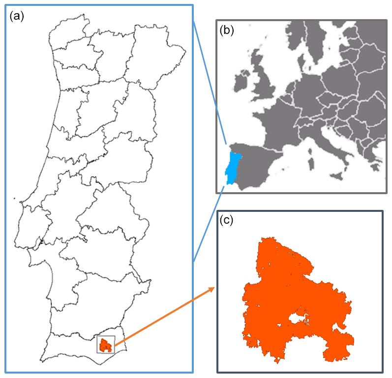
Figure 1(a) Map of Portugal with the location of the Tavira wildfire, where orange represents the burned scar and the black frame indicates the study area used in the simulations. (b, c) Schematic representation of Europe with Portugal highlighted in blue (b) and a zoom of the study area (c).
The fire propagated in two distinct phases. In the first stage, from 13:00 UTC on 18 July to 17:00 UTC on 19 July, the fire burned about 5,000 ha, representing one-fifth of the total burned area. In this phase, the wind direction was highly variable and the fire advanced through rugged terrain, with frequent shifts in the direction of maximum spread until it reached the Leiteijo stream.
In the second stage from 17:00 to 24:00 UTC on 19 July the fire turned into a major conflagration, greatly increasing its propagation speed and burning about 20 000 ha in 7 h. When the fire reached the Odeleite stream it became orographically channeled, as an increase in wind speed led to fast and intense fire growth towards the south, where heavy fuel loads were present. The fire split into two advanced sections heading west and east to the São Brás de Alportel and the Tavira municipalities, with a 10 km wide fire front. In addition, spotting created new fires up to 2 km ahead of the fire front. All these factors allowed rapid propagation of the fire front while making suppression extremely difficult.
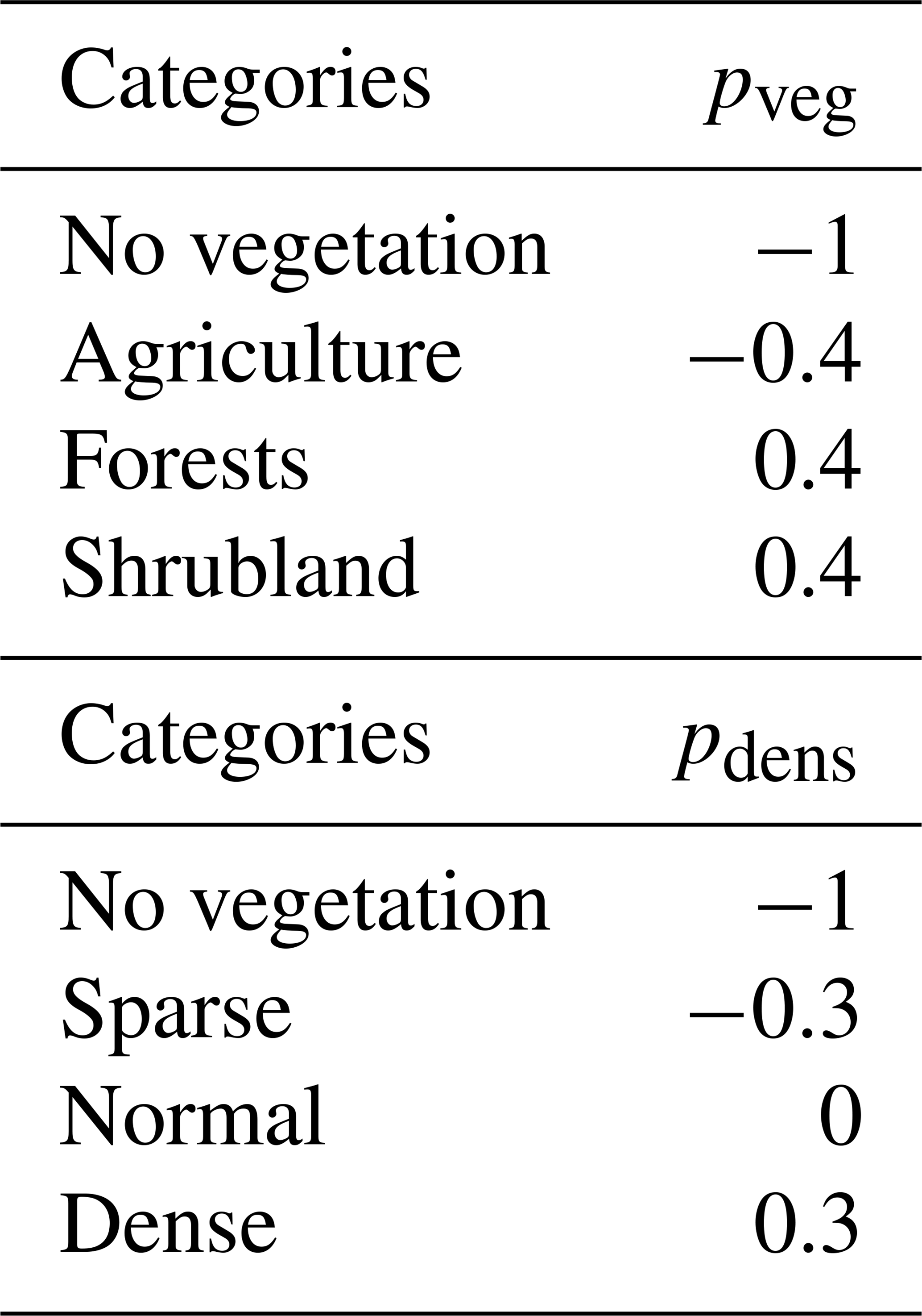
Table 1Assigned values to loadings of vegetation type (pveg) and density (pdens).
2.2 Input data
A study area of 30 km × 30 km was defined centered on the burned area (Fig. 1) and fine-scaled raster data from various sources were collected and preprocessed in a common format suitable as input for the wildfire simulations. Data include the ignition points, the start and end times of the fire event, the fire perimeters, the burned areas, the surface wind speed and direction, the topography, and information about the land cover (vegetation type, vegetation density, areas burnt in previous wildfires, waterlines and roads).
Patch-slope information was derived from elevation data as obtained from the digital elevation model provided by the Shuttle Radar Topography Mission (Farr et al., 2007).
Hourly wind data were obtained from a regional weather simulation performed with the Weather Research and Forecasting (WRF) model, version 3.1.1 (Skamarock et al., 2008). The quality of the simulation was previously assessed for wind (Cardoso et al., 2012; Soares et al., 2014). WindNinja (version 2.1.3) (Forthofer, 2007) was then used to spatially model the hourly wind input data taking into account the interaction with topography. The temporal behavior of the wind field was then validated against the information contained in the report by the Portuguese Institute for Nature Conservation and Forests (ICNF) (ICNF, 2012).
Fuel type and density were derived by combining information from CORINE Land Cover raster maps at 100 m resolution (CLC2006, 2019), the National Forest Inventories produced by ICNF and the MODIS-based annual maximum green vegetation fraction (Broxton et al., 2014). Vegetation types were aggregated into four main categories: areas without vegetation, agriculture, shrubland and forests (Fig. 2a). The density of vegetation was also stratified into four categories: areas without vegetation and areas with sparse, normal and dense vegetation (Fig. 2b). As described in Sect. 2.3, for the different categories of vegetation type and density, values of the associated loadings, respectively pveg and pden, were empirically assigned or taken from literature (Alexandridis et al., 2008). Assigned values are listed in Table 1.
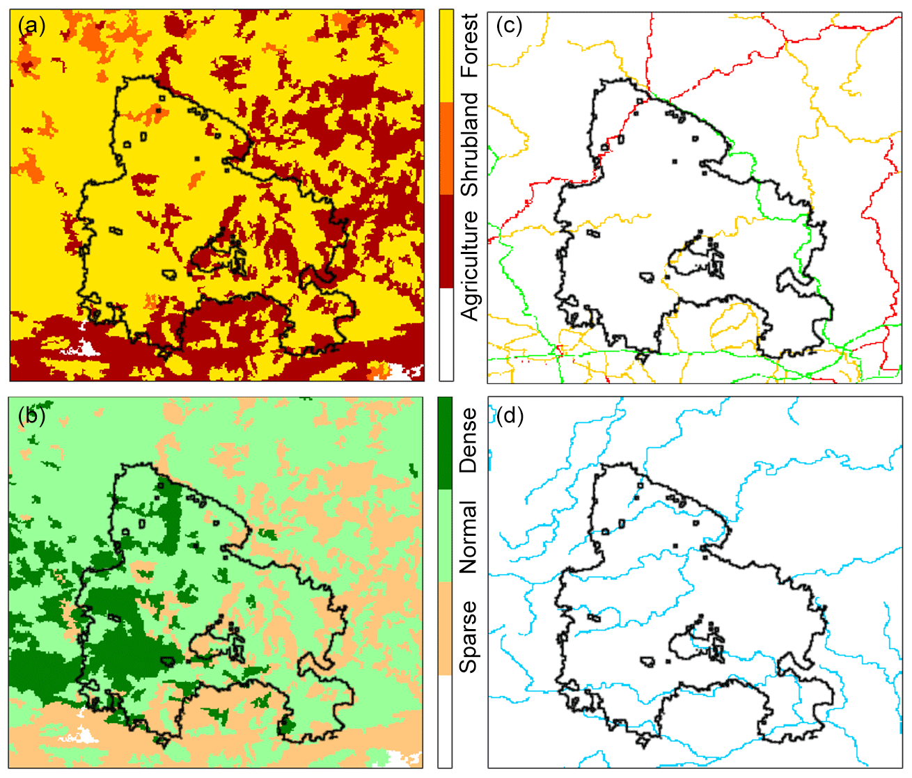
Figure 2(a, b) Vegetation type (a) and density classes (b) inside the study area as indicated by the discrete color bars. White corresponds to areas without vegetation. (c, d) The roads (c) and waterlines (d) identified inside the simulation area. Primary, secondary and tertiary roads are represented, respectively, in red, orange and green. Waterlines are all colored in blue.
Roads and waterlines inside the simulation area (Fig. 2c and d) were also included in the model by assigning low values to loadings of both pveg and pdens, with pveg=pdens. Primary, secondary and tertiary roads were assigned the values −0.8, −0.7 and −0.4, respectively, whereas the value of −0.4 was assigned to the waterlines.
Active fire data as identified from satellites were used for the quality assessment of the CA model simulations by evaluating temporal and spatial discrepancies between active fire observations and simulated fire growth. For this purpose, we used the MODIS (MODerate Resolution Imaging Spectroradiometer) active fire product that provides hot spots detected at 1 km × 1 km pixel resolution, at the time of the satellite overpass. The MODIS sensor on the Terra and Aqua satellites supplies daytime and nighttime observations at four nominal acquisition times, thus providing information about the geographical location, date and time of the detected active fires (Giglio et al., 2003).
For each satellite overpass totally or partially covering the total burned area by the Tavira fire, we used the centroids of the active fire footprints (Fig. 3a) to define a polygon confined to the burn scar. Times of burning of cells inside the fire scar were then estimated by bilinearly interpolating among the outer limits of the defined polygons (Fig. 3b).

Figure 3Centroids of the active fires detected by MODIS (a) and derived times of burning for the cells inside the burned scar (b). Colors of the centroids and of the cells represent the elapsed time (in hours) since the beginning of the fire event as indicated in the color bars. The star represents the fire ignition point reported and the black line the perimeter of the burned area.
2.3 Baseline model
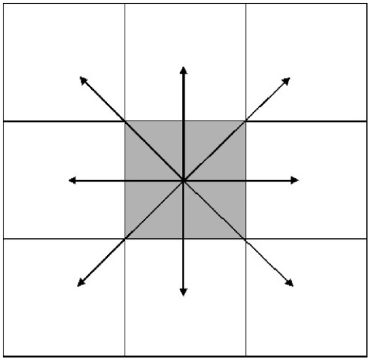
Simulations by the reference CA model developed by Alexandridis et al. (2008) make use of a square grid with propagation to the eight nearest and next-nearest neighbors (Fig. 4). Each cell (or site) is characterized by four possible discrete states, corresponding to burning, with fuel not yet burned, fuel free and completely burned cells. The model has four possible rules of evolution that take into account fuel properties, wind conditions and topography. The rules are applied at each time step and are described as follows. Rule 1 states a cell that cannot be burned stays the same. Rule 2 states a cell that is burning down at present time will be completely burned in the next time step. Rule 3 states a burned cell cannot burn again. Rule 4 states if a cell is burning down at the present time and there are next-nearest neighbor cells containing vegetation fuel, then the fire can propagate to its neighbors with a probability pburn, which is a function of the variables that affect fire spread.
Probability pburn of a given cell depends on a constant reference probability that may be increased or decreased by means of different loadings. The constant reference probability p0 is the probability that a cell in the neighborhood of a burning cell (containing a given type of vegetation and density) starts burning at the next time step under no wind and flat terrain. Loadings in turn depend on the vegetation type, pveg, and vegetation density, pden; on topography, ps; and on wind fields, pw. In its basic formulation pburn is set as
As described in Sect. 2.2, in order to account for the effect of vegetation, both type and density were stratified into discrete classes, and for each class a constant loading was assigned as specified in Table 1.
The effect of the wind is modeled as
where c1 and c2 are adjustable coefficients, V is the wind speed, and θ is the angle between the wind direction and the fire propagation direction. As expected, pw increases when wind and fire directions are aligned.
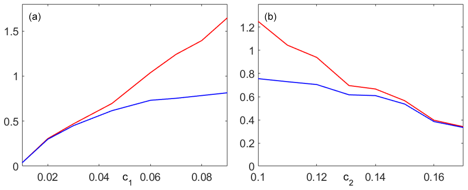
Figure 6Simulated values of the total burned area (red curves) and of the burned area inside the perimeter of the fire scar (blue curves) in units of the total area inside the perimeter as a function of c1 for fixed c2=0.131 (a) and as a function of c2 for a fixed c1=0.045 (b).
The probability factor that models the effect of the terrain slope is given by
where θs is the slope angle of the terrain and as is a coefficient that can be adjusted from experimental data. Slope angle θs was derived from elevation data, E, according to
where D is equal to the size L of the square cell when the two neighboring cells are adjacent to when the two cells are diagonal. As expected this topography effect is higher when the fire spreads uphill.
2.4 Modified model
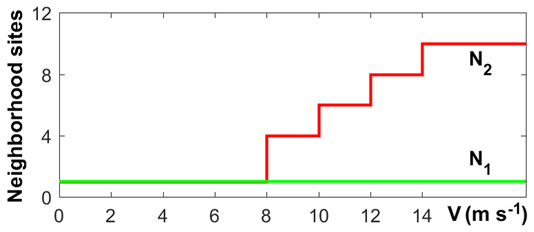
In order to better mirror the role played by the wind in fire propagation, a modification was introduced in the model by means of a new rule that allows propagation to nonadjacent cells with the aim of incorporating the effects due to fire spotting (Fig. 5). In contrast with the baseline rule N1 that at each time step fire can only spread to its nearest and next-nearest neighbors, according to the new rule N2, for each burning cell at a given time step, fire propagation is modeled according to the two following steps: apply the baseline wind rule and determine the direction(s) of fire spread (if any) for each cell in the next-nearest neighborhood. If (i) according to the previous step, the fire propagates to a new cell, (ii) the wind speed at the considered burning cell is above the threshold of 8 m s−1 and (iii) the angle between the wind direction and the displacement vector (from the considered burning cell to the newly ignited cell) is lower than π∕10, then fire also spreads to a number of other contiguous cells (along the displacement vector), with the number of ignited cells depending on the wind speed at the considered burning cell (Fig. 5).
The model with the new propagation rule N2 will be hereafter referred to as the modified model.
2.5 Simulations
The landscape was discretized into square cells with sizes of 100 m and the model free parameters were set according to Alexandridis et al. (2008), i.e., with p0=0.58, as=0.078, c1=0.045 and c2=0.131. The time step of the model was set by performing 100 simulations of the propagation of fire inside the observed burned area under no-wind and flat-terrain conditions. The time step was then estimated by dividing the observed time from the starting ignition up to fire containment (46 h) by the mean number of time steps required to burn the entire area. The obtained time step was about 20 min.
A sensitivity study was also performed to assess the effects of constants c1 and c2 on the propagation of fire (Eq. 2). As shown in Fig. 6, simulated values of total burned area and of burned area inside the perimeter of the fire scar increase (decrease) with increasing c1 (increasing c2). Moreover, above (below) a certain threshold of c1 (c2), a progressive departure is observed between the simulated values of total burned area and of burned area inside the perimeter of the fire scar, an indication that the simulated fire is spreading out of the recorded limits. Choice of c1=0.045 and c2=0.131 (Alexandridis et al., 2008) represents a compromise between burning a large fraction of the area inside the perimeter and spreading a small fraction outside.
The fire event was then modeled using a probabilistic approach based on ensembles of 100 model simulations and the probability that a given cell burns was accordingly estimated by the fraction of runs in which that cell was modeled as a burned one. Two different kinds of simulations were performed, constrained and unconstrained. In the first kind, burning was confined to the observed burned area by means of an appropriate setting of the model parameters along the boundary of the final observed scar. It may be noted that this setting along the scar boundary is not an artificial device since it reflects the known a posteriori fact that the shape of the scar resulted from effective firefighting in locations where changes in fuel types and the presence of roads make fire propagation harder. In the second kind of simulations, no other constraints were imposed other than the lattice.

Figure 7Probabilities of burning (%) for the baseline model (a) and for the modified model (b). Colors represent the percentage of burned cells as indicated by the color bar in the bottom of the figure and white represents unburned cells. The star locates the fire ignition point, the blue line is the perimeter of the burned area and the green circles represent active fires as detected by MODIS. Both simulations were restricted to the burned area.

Figure 8Fraction of the burned area inside the perimeter relative to the total area inside the perimeter of the fire scar (a), bias (b) and root-mean-square difference (c) as a function of the probability threshold for c1=0.045 and c2=0.131. The dashed lines correspond to the baseline model and the solid lines to the modified model.
3.1 Constrained runs
Two different ensembles of 100 simulations were generated, one with the baseline fire spread model and the other with the modified model. Results obtained at four selected stages of the fire are displayed in Fig. 7. When using the baseline rule (Fig. 7a), and except for the slot at 25 h (after ignition) where there is a fair agreement between the simulated burned area and the front lines of the fire as indicated by the hot spots identified by satellite, the simulated burning is well behind the fire front, an indication that the modeled propagation of the fire is too slow. A strong contrast is observed when using the modified model (Fig. 7b). In this case, the modeled burned areas spread much closer to the fire front as defined by the hot spots. The exception is the slot at 25 h (after ignition), where the modeled propagation of fire is faster than the one suggested by the location of the hot spots. Conversely, it is worth emphasizing that the explosive behavior of fire between slots at 25 and 33 h is well simulated when using the new wind propagation rule.
Burned area in each one of the two ensembles was identified by assuming that a given pixel is a burned one when the modeled probability that it burned is larger than a fixed threshold. Each pixel identified as burned was assigned the respective time step as an indicator of the modeled time of burning. Time deviations were then computed by subtracting the times of burning as derived from the hot spots identified by MODIS (Fig. 3b). Finally, three measures of quality of the simulations were derived for different thresholds of probability, namely the fraction of burned area (relative to the total area inside the perimeter of the fire scar), the bias (simulated time minus time derived from hot spots) and root-mean-squared differences (between simulated time and time derived from hot spots).
Figure 8 presents results obtained when using the model with the baseline wind rule (dashed lines) and the modified model (solid lines). In both cases, and as to be expected, the fraction of burned area decreases with increasing values of the threshold (Fig. 8a), with the baseline model always presenting, for each threshold, lower values of burned area than the modified model. The baseline (modified) model presents positive (negative) values of bias for each threshold (Fig. 8b), meaning that, on average, the simulations are late (in advance) when compared with times derived from satellites. In both cases, the bias increases with increasing values of threshold, with the baseline model becoming more and more biased and the modified model approaching zero bias, although the rate of increase is smaller than the one of the baseline model. Finally, the root-mean-square difference (Fig. 8c) shows an opposite behavior in the two cases, with values increasing (decreasing) with the threshold in the case of the baseline (modified) model. When considering all together the three measures of quality of the simulations, the modified one performs better than the baseline model and choosing values of threshold between 0.4 and 0.6 represents a good compromise in terms of simulated burned area and simulated time of fire propagation.
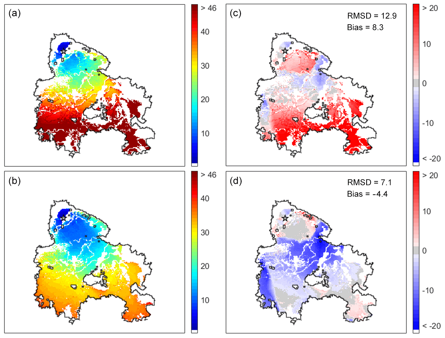
Figure 9(a, b) Fire propagation using a threshold of 0.5 for probability of burning for a set of 100 random simulations of the baseline model confined to the burned area (a) and of the modified model (b). Colors represent the elapsed time in hours after the fire ignites. (c, d) Time deviations from the left panels relative to the active fires detected by MODIS. Red (blue) shading corresponds to a progressive delay (advance) in fire propagation observed in the CA model, and light gray corresponds to an agreement between the CA model and the MODIS active fires. The star represents the fire ignition point, the black line the perimeter of the burned area and white the unburned cells.
Figure 9 presents the spatial distribution of fire propagation and of time deviations (simulated time minus time derived from hot spots) for a probability threshold of 0.5. When using the baseline wind rule (Fig. 9, upper panels), the model shows a progressive delay in the propagation of fire, with the isochrones of fire propagation attaining values larger than 46 h well before the fire front reaches the southern boundary of the scar. This delay is reflected in the positive values of the deviations of modeled time of burning from the one derived from satellite observations and it is worth noting that the delay takes place during the explosive stage of the fire between 25 and 33 h (Fig. 3b). When using the modified model (Fig. 9, lower panels) the explosive stage of the fire is much better modeled, albeit there is a too fast propagation of the fire front during the first stage. This behavior is reflected in the deviations that present negative values during the first 12 h and much lower positive values than the baseline model between 25 and 33 h, an indication that the modified model tends to be closer to the observations than the baseline model. The overall behavior of both models is well summarized by the respective values of bias and of root-mean-square differences: bias of 8.3 h (−4.4 h) of the baseline model (modified model) is consistent with the too slow (too fast) propagation of the modeled fire fronts whereas the root-mean-square difference of 12.9 h (7.1 h) points to a behavior closer to observations of the modified model.
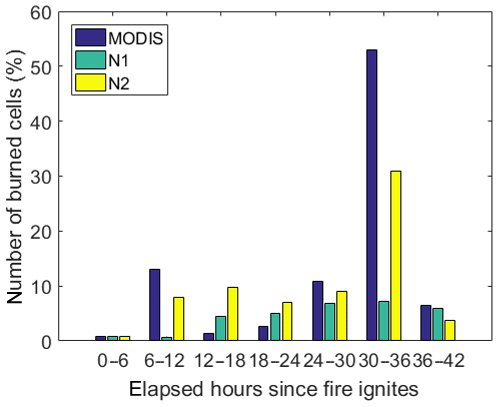
Figure 10Percentage of the total number of burned cells as derived from active fires (MODIS), the baseline model (N1) and the modified model (N2). Each triplet of columns corresponds to the burned cells identified in the intervals [0, 6[, [6, 12[, [12, 18[, [18, 24[, [24, 30[, [30, 36[ and [36, 42[ h.
The improved behavior of the modified model when compared with the baseline model is also revealed when analyzing the fraction of burned pixels of the scar in successive periods of 6 h (Fig. 10). The most conspicuous feature is the burning of more than 50 % of the total amount of burned cells between 30 and 36 h. This explosive stage of the fire is completely missed by the baseline model, whereas the burned area by the modified model reaches 30 %. When the fraction of burned area estimated from remotely sensed hot spots is small (between 0 and 6, 12 and 18, 18 and 24 h) both models tend to overestimate that fraction, especially the modified model. Between 6 and 12 h, the burned fraction simulated by the modified model is close to the burned area estimated from hot spots, whereas the baseline model underestimates that fraction. An opposite behavior occurs in the last interval, between 36 and 42 h, when the fraction simulated by the baseline is close to the fraction estimated from hot spots and the modified model underestimates that fraction.
3.2 Unconstrained runs
When no constraints are imposed, the obtained pattern of burning probabilities (Fig. 11a) shows a marked decrease outside the limits of the burned scar and this may be shown by restricting the burned area to cells with a burning probability larger than 80 % (Fig. 11b). Unconstrained simulations therefore indicate that the probability of burning is lower beyond the actual perimeter of the fire scar as a result of changes in fuel type, topographic effects and the presence of linear interruptions such as roads.
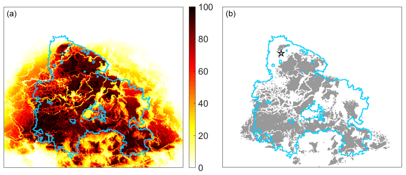
Figure 11(a) Probabilities of burning (%) as derived from an ensemble of 100 unconstrained simulations of the modified model. The color bar indicates the probability of burning. The star represents the fire ignition point, the black line the perimeter of the burned area and white the unburned cells. (b) Burned sites identified above a threshold probability of 80 %. The blue arrows indicate locations where fire fighting occurred, namely along the lateral sides of the burned scar and populated areas.
Two different ensembles of constrained runs were generated, based on two models that were analogous except in the wind propagation rule. In the baseline model, the wind rule only applied to the nearest and next-nearest neighbors, whereas in the modified model the neighborhood affected increased with wind speed, reaching up to 10 cells. Results obtained pointed to a progressive delay in the propagation of fire simulated by the baseline model that contrasted with a moderate advance obtained with the simulations by the modified model. The contrast in overall behavior of the two ensembles is reflected in the obtained values of bias and root-mean-square deviations between simulated times of burning of each cell and respective estimated times from hot spots as identified by remote sensing. The value of 8.3 h (−4.4 h) for bias in the case of the baseline (modified) model indicates the overall delay (advance) of the simulation, and the improved performance of the modified model is suggested by the value of 7.1 h of the root-mean-square difference that is more than 2 h lower than the value of 12.9 h obtained with the baseline model. Differences between the two ensembles are conspicuous during the explosive stage of the wildfire when about 55 % of the area burned between 30 and 36 h after the fire onset. The baseline model simulated less than 10 % (out of 55 %) of that area whereas the modified model reached 30 %. The usefulness of the modified model as a tool to assist fire managers in locating resources for firefighting during a fire event was tested by performing a third ensemble of 100 simulations in which the fire propagation is unconstrained and the simulations stop by themselves. Results obtained show a marked decrease in probability of burning outside the observed fire scar, suggesting that this type of model may help decision-makers allocate firefighting forces during a real fire event (Fig. 11b).
The flexibility to the introduction of changes in properties of individual cells (e.g., when imposing constraints to fire propagation along the perimeter of the fire scar) as well as of transition rules (e.g., the proposed one on the effects of wind), together with the required low computational cost (that allows us to perform a very large number of runs in a short amount of time), make CA adequate tools to be used, when either planning controlled fires or making decisions about fighting in an operational scenario. For instance, we are currently developing a mobile application (app) that allows the user to run the proposed modified model over the study area and modify the properties of the individual cells.
In this paper we set up a CA model designed to respond to wind-driven wildfires. The model is applied to a large wildfire event that took place in southern Portugal in July 2012. In addition to its relevance in terms of burned area that reached almost 25 000 ha, the event turned into a major conflagration between 25 and 33 h after the onset because of orographic channeling accompanied by an increase in wind speed. This explosive stage represented an ideal scenario to test a CA model designed for wind-driven wildfires. The simulation of the wildfire propagation was made using a probabilistic approach based on ensembles of 100 simulations that allows estimation of the probability of burning of a given cell by the fraction of runs in which that cell was modeled as a burned one.
The proposed CA model with a wind rule that allows fire propagation to nonadjacent cells represents an improvement to the baseline model and reveals potential to be an added value in fire management. In addition to introducing the effect of fire spotting, the new wind rule is also an attempt to circumvent the problem of having a fixed time step for the propagation of fire on a fixed lattice. Results indicate that unconstrained simulations are a useful tool to assist decision-makers during a fire event by providing indications about locations of low burning probability to be selected as appropriate for allocating resources for fire fighting. Currently the model is being tested in different scenarios, namely with the very large fire events that took place in Portugal in June and October 2017.
It is worth mentioning that the transition rules that were used in the CA model do not take into consideration either the state of stress of vegetation or the meteorological conditions. In line with Alexandridis et al. (2011), incorporation of these two aspects is currently being considered by associating probability factors with the Drought Code (DC) and with the Fine Fuel Moisture Code (FFMC), two indices of the Canadian Fire Weather Index System that respectively provide a numerical rating of seasonal drought effects and of the ease of ignition, and the flammability of fine fuel at the daily level (Pinto et al., 2018; Wagner, 1974, 1987).
Finally, it may be noted that results from the CA models are presented in terms of probability of burning as an outcome of ensembles of runs. This raises the issue of providing information of model uncertainty that is especially relevant if the CA model is to be used as a decision-making support tool. As discussed in Fischhoff and Davis (2014), characterizing model uncertainty involves identifying key outcomes, characterizing variability as well as internal and external validity, and finally summarizing uncertainty. Presentation of the impacts on fraction of burned area, bias and root-mean-square deviations when choosing different thresholds of probability of burning is a first step towards conveying results of uncertainty. Further steps in this direction will have to involve direct contact with decision-makers when analyzing other large fire events, namely the abovementioned ones that took place in Portugal in June and October 2017.
The used datasets are publicly available at the following links: https://land.copernicus.eu/pan-european/corine-land-cover/clc-2006 (last access: 17 January 2019), https://archive.usgs.gov/archive/sites/landcover.usgs.gov/green_veg.html (last access: 17 January 2019) and https://search.earthdata.nasa.gov (last access: 17 January 2019).
JGF performed the study. JGF and CDC wrote the paper, discussed the results and reviewed the paper.
The authors declare that they have no conflict of interest.
This article is part of the special issue “Spatial and temporal patterns of wildfires: models, theory, and reality”. It is a result of the conference EGU 2017, Vienna, Austria, 23–28 April 2017.
Joana Gouveia Freire was supported by the postdoctoral grant SFRH/BPD/101760/2014 from FCT,
Portugal. Part of this work was also supported by the project BrFLAS – Brazilian
Fire-Land-Atmosphere System (FAPESP/1389/2014) funded by national
funds through the Portuguese Foundation for Science and Technology (FCT).
Part of the data were provided by the FIRE-MODSAT project, financed by FCT,
Portugal (contract EXPL/AGR-FOR/0488/2013).
Edited by: Marj Tonini
Reviewed by: three anonymous referees
Alexandridis, A., Vakalis, D., Siettos, C. I., and Bafas, G. V.: A Cellular Automata model for forest fire spread prediction: The case of the wildfire that swept through Spetses Island in 1990, Appl. Math. Comput., 204, 191–201, https://doi.org/10.1016/j.amc.2008.06.046, 2008. a, b, c, d, e
Alexandridis, A., Russo, L., Vakalis, D., Bafas, G. V., and Siettos, C. I.: Wildland fire spread modelling using cellular automata: evolution in large-scale spatially heterogeneous environments under fire suppresion tactics, Int. J. Wildland Fire, 20, 633–647, https://doi.org/10.1071/WF09119, 2011. a, b, c
Amraoui, M., Liberato, M. L. R., Calado, T. J., DaCamara, C. C., Coelho, L. P., Trigo, R. M., and Gouveia, C. M.: Fire activity over Mediterranean Europe based on information from Meteosat-8, Forest Ecol. Manage., 294, 62–75, https://doi.org/10.1016/j.foreco.2012.08.032, 2013. a
Amraoui, M., Pereira, M. G., DaCamara, C. C., and Calado, T. J.: Atmospheric conditions associated with extreme fire activity in the Western Mediterranean region, Sci. Total Environ., 524-525, 32–39, https://doi.org/10.1016/j.scitotenv.2015.04.032, 2015. a
ANPC: Tavira/Cachopo/Catraia ocurrence report 2012080021067, National Authority for Civil Protection, available at: https://www.bombeiros.pt/wp-content/uploads/2012/09/Relatorio-de-ocorrencia-2012080021067-Tavira_Cachopo_Catraia.pdf (last access: 17 January 2018), 2012. a
Broxton, P. D., Zeng, X., Scheftic, W., and Troch, P. A.: A MODIS-Based 1 km Maximum Green Vegetation Fraction Dataset, J. Appl. Meteorol. Clim., 53, 1996–2004, https://doi.org/10.1175/JAMC-D-13-0356.1, 2014. a
Cardoso, R. M., Soares, P. M. M., Miranda, P. M. A., and Belo-Pereira, M.: WRF high resolution simulation of Iberian mean and extreme precipitation climate, Int. J. Climatol., 33, 2591–2608, https://doi.org/10.1002/joc.3616, 2012. a
Clarke, K. C., Brass, J. A., and Riggan, P. J.: A Cellular Automaton Model of Wildfire Propagation and Extinction, Photogram. Eng. Remote Sens., 60, 1355–1367, 1994. a
CLC2006: The CORINE Land Cover (CLC) dataset produced in 2006, available at: https://land.copernicus.eu/pan-european/corine-land-cover/clc-2006 (last access: 17 January 2018), 2019. a
Collin, A., Bernardin, D., and Séro-Guillaume, O.: A physical-based cellular automaton model for forest-fire propagation, Combust. Sci. Technol., 183, 347–369, https://doi.org/10.1080/00102202.2010.508476, 2011. a
DaCamara, C. C., Calado, T. J., Ermida, S. L., Trigo, I. F., Amraoui, M., and Turkman, K. F.: Calibration of the Fire Weather Index over Mediterranean Europe based on fire activity retrieved from MSG satellite imagery, Int. J. Wildland Fire, 23, 945–958, https://doi.org/10.1071/WF13157, 2014. a
Farr, T. G., Rosen, P. A., Caro, E., Crippen, R., Duren, R., Hensley, S., Kobrick, M., Paller, M., Rodriguez, E., Roth, L., Seal, D., Shaffer, S., Shimada, J., Umland, J., Werner, M., Oskin, M., Burbank, D., and Alsdorf, D.: The shuttle radar topography mission, Rev. Geophys., 45, RG2004, https://doi.org/10.1029/2005RG000183, 2007. a
Finney, M. A.: FARSITE: fire area simulator – model development and evaluation, Research Paper RMRS-RP-4 Revised, US Department of Agriculture, Forest Service, Rocky Mountain Research Station, Ogden, UT, 47 pp., 2004. a
Fischhoff, B. and Davis, A. L.: Communicating scientific uncertainty, P. Natl. Acad. Sci. USA, 111, 13664–13671, https://doi.org/10.1073/pnas.1317504111, 2014. a
Forthofer, J. M.: Modeling Wind in Complex Terrain for use in Fire Spread Prediction, Thesis, Colorado State University, Fort Collins, CO, 123 pp., 2007. a
Ghisu, T., Arca, B., Pellizzaro, G., and Duce, P.: An Improved Cellular Automata for Wildfire Spread, Proced. Comput. Sci., 51, 2287–2296, https://doi.org/10.1016/j.procs.2015.05.388, 2015. a
Giglio, L., Descloitres, J., Justice, C. O., and Kaufman, Y.: An enhanced contextual fire detection algorithm for MODIS, Remote Sens. Environ., 87, 273–282, https://doi.org/10.1029/2005JG000142, 2003. a
ICNF: Recuperação da área ardida do incêndio de Catraia, Tech. report, available at: http://www2.icnf.pt/portal/florestas/dfci/relat/raa/rel-tec/raai-catraia-2012 (last access: 17 January 2018), 2012. a, b
Panisset, J., DaCamara, C. C., Libonati, R., Peres, L. F., Calado, T. J., and Barros, A.: Effects of regional climate change on rural fires in Portugal, Anais da Academia Brasileira de Ciências (Annals of the Brazilian Academy of Sciences), 89, 1487–1501, https://doi.org/10.1590/0001-3765201720160707, 2017. a
Pereira, M. G., Trigo, R. M., DaCamara, C. C., Pereira, J. M. C., and Leite, S. M.: Synoptic patterns associated with large summer forest fires in Portugal, Agr. Forest Meteorol., 129, 11–25, https://doi.org/10.1016/j.agrformet.2004.12.007, 2005. a
Pereira, M. G., Calado, T. J., DaCamara, C. C., and Calheiros, T.: Effects of regional climate change on rural fires in Portugal, Clim. Res., 57, 187–200, https://doi.org/10.3354/cr01176, 2013. a
Pinto, M. M., DaCamara, C. C., Trigo, I. F., Trigo, R. M., and Turkman, K. F.: Fire danger rating over Mediterranean Europe based on fire radiative power derived from Meteosat, Nat. Hazards Earth Syst. Sci., 18, 515–529, https://doi.org/10.5194/nhess-18-515-2018, 2018. a
Pinto, R. M. S., Benali, A., Sá, A. C. L., Fernandes, P. M., Soares, P. M. M., Cardoso, R. M., Trigo, R. M., and Pereira, J. M. C.: Probabilistic fire spread forecast as a management tool in an operational setting, SpringerPlus, 5, 1205, https://doi.org/10.1186/s40064-016-2842-9, 2016. a
Rothermel, R. C.: A mathematical Model for predicting fire spread in wildland fuels, Research Paper INT-115, US Department of Agriculture, Forest Service, Intermountain Forest and Range Experiment Station, Ogden, UT, 47 pp., 1972. a
Rothermel, R. C.: How to predict the spread and intensity of forest fire and range fires, General Technical Report INT-143, US Department of Agriculture, Forest Service, Intermountain Forest and Range Experiment Station, Ogden, UT, 161 pp., 1983. a
Rui, X., Hui, S., Yu, X., Zhang, G., and Wu, B.: A physical-based cellular automaton model for forest-fire propagation, Nat. Hazards, 91, 309–319, https://doi.org/10.1007/s11069-017-3127-5, 2018. a
San-Miguel-Ayanz, J., Durrant, T., Boca, R., Libertà, G., Branco, A., de Rigo, D., Ferrari, D., Maianti, P., Vivancos, T. A., Costa, H., Lana, F., Löffler, P., Nuijten, D., Ahlgren, A. C., and Leray, T.: Forest Fires in Europe, Middle East and North Africa 2017, https://doi.org/10.2760/663443, 2017. a
Skamarock, W. C., Klemp, J. B., Dudhia, J., Gill, D. O., Barker, D. M., Duda, M. G., Huang, X.-Y., Wang, W., and Powers, J. G.: A description of the Advanced Research WRF version 3, NCAR Tech. Note NCAR/TN-475+STR, NCAR, https://doi.org/10.5065/D68S4MVH, 2008. a
Soares, P. M. M., Cardoso, R. M., Semedo, A., Chinita, M. J., and Ranjha, R.: Climatology of Iberia coastal low-level wind jet: WRF high resolution results, Tellus A, 66, 22377, https://doi.org/10.3402/tellusa.v66.22377, 2014. a
Sullivan, A. L.: Wildland surface fire spread modelling, 1990–2007. 3: Simulation and mathematical analogue models, Int. J. Wildland Fire, 18, 387–403, https://doi.org/10.1071/WF06144, 2009. a, b
Trigo, R. M., Pereira, J. M. C., Pereira, M. G., Mota, B., Calado, M. T., DaCamara, C. C., and Santo, F. E.: Atmospheric conditions associated with the exceptional fire season of 2003 in Portugal, Int. J. Climatol., 26, 1741–1757, https://doi.org/10.1002/joc.1333, 2005. a
Trigo, R. M., Añel, J., Barriopedro, D., García-Herrera, R., Gimeno, L., Nieto, R., Castillo, R., Allen, M. R., and Massey, N.: The record Winter drought of 2011–2012 in the Iberian Peninsula, B. Am. Meteorol. Soc., 94, S41–S45, 2013. a
Trunfio, G. A.: Predicting wildfire spreading through a hexagonal cellular automata model, in: Lecture Notes in Computer Sciences, ACRI 2004, vol. 3305, edited by: Sloot, P. M. A. and Chopard, A. G. H., Springer-Verlag, Berlin, Heidelberg, 385–394, https://doi.org/10.1007/978-3-540-30479-1_40, 2004. a
Trunfio, G. A., D'Ambrosio, D., Rongo, R., Spataro, W., and Gregório, S. D.: A new algorithm for simulating wildfire spread through cellular automata, ACM T. Model. Comput. Simul., 22, 6, https://doi.org/10.1145/2043635.2043641, 2011. a
Viegas, D. X., Figueiredo, A. R., Ribeiro, L. M., Almeida, M., Viegas, M. T., Oliveira, R., and Raposo, J. R.: Tavira/São Brás de Alportel forest fire report 18–22 July 2012, available at: https://www.portugal.gov.pt/media/730414/rel_incendio_florestal_tavira_jul2012.pdf (last access: 17 January 2018), 2012. a
Wagner, C. E. V.: Structure of the Canadian Forest Fire Weather Index, Can. Forestry Serv., Publication 1333, Ottawa, Ontario, 49 pp., available at: http://www.cfs.nrcan.gc.ca/bookstore_pdfs/24864.pdf (last access: 17 January 2018), 1974. a
Wagner, C. E. V.: Development and structure of the Canadian Forest Fire Weather Index System, Can. Forestry Serv., Technical Report 35, Ottawa, Ontario, 48 pp., 1987. a