the Creative Commons Attribution 4.0 License.
the Creative Commons Attribution 4.0 License.
 | 23 Aug 2019
The impact of lightning and radar reflectivity factor data assimilation on the very short-term rainfall forecasts of RAMS@ISAC: application to two case studies in Italy
Rosa Claudia Torcasio
Elenio Avolio
Olivier Caumont
Mario Montopoli
Luca Baldini
Gianfranco Vulpiani
Stefano Dietrich
In this paper, we study the impact of lightning and radar reflectivity factor data assimilation on the precipitation VSF (very short-term forecast, 3 h in this study) for two severe weather events that occurred in Italy. The first case refers to a moderate and localized rainfall over central Italy that occurred on 16 September 2017. The second case occurred on 9 and 10 September 2017 and was very intense and caused damages in several geographical areas, especially in Livorno (Tuscany) where nine people died.
The first case study was missed by several operational forecasts, including that performed by the model used in this paper, while the Livorno case was partially predicted by operational models.
We use the RAMS@ISAC model (Regional Atmospheric Modelling System at Institute for Atmospheric Sciences and Climate of the Italian National Research Council), whose 3D-Var extension to the assimilation of radar reflectivity factor is shown in this paper for the first time.
Results for the two cases show that the assimilation of lightning and radar reflectivity factor, especially when used together, have a significant and positive impact on the precipitation forecast. For specific time intervals, the data assimilation is of practical importance for civil protection purposes because it changes a missed forecast of intense precipitation (≥40 mm in 3 h) to a correct one.
While there is an improvement of the rainfall VSF thanks to the lightning and radar reflectivity factor data assimilation, its usefulness is partially reduced by the increase in false alarms, especially when both datasets are assimilated.
- Article
(15031 KB) -
Supplement
(5734 KB) - BibTeX
- EndNote


Initial conditions of numerical weather prediction (NWP) models are a key point for a good forecast (Stensrud and Fritsch, 1994; Alexander et al., 1999). Today limited-area models are operational at the kilometric scale (< 5 km) and data assimilation of observations with high spatio-temporal resolution as lightning or radar reflectivity factor1 is crucial to correctly represent the state of the atmosphere at local scale (Weisman et al., 1997; Weygandt et al., 2008).
The assimilation of radar reflectivity factor is useful to improve the weather forecast considering the high spatio-temporal resolution of radar data.
First attempts to assimilate radar reflectivity factor are reported in Sun and Crook (1997, 1998), who expanded VDRAS (Variational Doppler Radar Analysis System) to include microphysical retrieval. Following these studies, several systems to assimilate radar observations, both Doppler velocity and reflectivity factor, were developed (Xue et al., 2003; Zhao et al., 2006; Xu et al., 2010). All these studies showed the stability and robustness of assimilating radar observations as well as the improvement of weather forecast.
In addition to direct methods, which assimilate the radar reflectivity factor adjusting the hydrometeor contents, there are indirect methods adjusting other variables. In particular, the method of Caumont et al. (2010) assimilates the relative humidity field. It consists of two different steps: a 1-D retrieval of relative humidity (pseudo-profile), which depends on the radar reflectivity factor observations, followed by 3D-Var assimilation of the pseudo-profile. This method has the advantage of reducing the computational cost at the kilometric scale.
The choice of updating the moisture field directly is motivated by its greater impact on analyses and forecasts in comparison to that of hydrometeor-related quantities (e.g. Fabry and Sun, 2010).
Caumont et al. (2010) showed that the method improved the weather prediction of a heavy precipitation event in southern France and of an 8 d long assimilation cycle experiment.
The method was applied in other studies (Wattrelot et al., 2014, using the AEROME model; Ridal and Dahlbom, 2017; using the HARMONIE model), or modified using 4D-Var in place of 3D-Var (Ikuta and Honda, 2011; using the JNoVa model), showing its capability to improve the weather forecast. The method is also used in the operational context (Wattrelot et al., 2014).
Lightning is another important source of asynoptic data due to its ability to precisely locate the convection with few temporal gaps (Mansell et al., 2007). In the last 2 decades, there have been attempts to assimilate lightning into meteorological models at both low horizontal resolution, which needs a cumulus parameterization scheme to simulate convection, and at convection-permitting scales.
First attempts to assimilate lightning in NWP models were based on relationships between lightning and rainfall rate estimated by microwave sensors on board polar-orbiting satellites (Alexander et al., 1999; Chang et al., 2001; Jones and Macpherson, 1997; Pessi and Businger, 2009). In this approach, the rainfall rate was computed as a function of the density of lightning observations and then transformed into latent heat, which was assimilated. The results of these studies showed a positive impact of the lightning data assimilation on the forecast up to 24 h also for fields at the large scale, such as sea-level pressure.
The study of Papadopoulos et al. (2005) used lightning to locate convection and the simulated water vapour profile was nudged towards vertical profiles recorded during convective events.
Mansell et al. (2007) modified the Kain–Fritsch (Kain and Fritsch, 1993) cumulus convective scheme to force convection when and where flashes are observed while the convection scheme was not activated in the model simulation, demonstrating the potential of lightning to improve the convection forecast. A similar approach was introduced by Giannaros et al. (2016) into WRF, showing the positive impact of lightning data assimilation on the precipitation forecast up to 24 h for eight convective events that occurred over Greece.
Fierro et al. (2012) introduced a methodology to assimilate lightning at convection-resolving scales by modifying the water vapour mixing ratio simulated by WRF according to a function depending on the flash rate and on the simulated graupel mixing ratio. The water vapour could be assimilated by nudging (Fierro et al., 2012) or 3D-Var (Fierro e al., 2016).
Qie et al. (2014), using WRF, adopted the methodology of Fierro et al. (2012) to assimilate ice crystals, graupel, and snow, showing promising results for deep convective events in China.
Fierro et al. (2015) studied the performance of the Fierro et al. (2012) method for 67 d spanning the 2013 warm season over the contiguous US, giving a statistically robust estimation of the performance of the method. The computationally inexpensive lightning data assimilation method improved the short-term (≤6 h) precipitation forecast of high impact weather considerably.
Lynn et al. (2015) and Lynn (2017) also applied the method of Fierro et al. (2012) to boost the local thermal buoyancy where and when lightning is observed. Results show that lightning data assimilation improved lightning forecast. Importantly, Lynn et al. (2015) offer an approach to address spurious convection (i.e. convection removal), which is a more challenging problem to tackle.
Federico et al. (2017a) implemented the methodology of Fierro et al. (2012) in the RAMS@ISAC model, showing the systematic and significant improvement of the precipitation forecast at the very short range (3 h) for 20 case studies that occurred over Italy; the impact of lightning data assimilation for longer forecast ranges (6–24 h; Federico et al., 2017b) showed a considerable impact on the 6 h precipitation forecast, with smaller (negligible) effects at 12 h (24 h).
In this paper, we study the impact of radar reflectivity factor and lightning data assimilation on the very short-term (3 h) rainfall prediction for two case studies in Italy. We use the method of Fierro et al. (2012) to assimilate lightning and the method of Caumont et al. (2010) to assimilate the radar reflectivity factor. The case studies occurred in September 2017. The first case, hereafter referred to as Serrano, occurred on 16 September and was characterized by moderate-intense and localized rainfall. The second case, hereafter referred to as Livorno, occurred on 9–10 September, and was characterized by deep convection and very intense precipitation in several parts of Italy. Even if the Livorno case occurred before the Serrano case, we reverse the chronological order in the discussion, ordering the event from the less to the most intense.
The forecast of severe events at the local scale still remains challenging because of the multitude of physical processes involved over a wide range of scales (Stensrud et al., 2009). The Serrano case study, being localized in space, poses challenges in forecasting the exact position and timing of convection initiation; the Livorno event involves the interaction between a high-impact storm and the complex orography of Italy, which is difficult to simulate at the local scale. For the above reasons the forecast of both events was challenging, as confirmed by the poor forecast of RAMS@ISAC without data assimilation. The difficulty to timely and accurately forecast the precipitation field for the two case studies is the reason for choosing them as test cases.
This paper presents for the first time the assimilation of the total lightning (intra-cloud + cloud to ground) and radar reflectivity factor in RAMS@ISAC and shows how the assimilation of radar reflectivity factor works together with total lightning data assimilation. Also, this paper shows that the precipitation forecast using cloud-scale observations over complex terrain can be accurate, contributing to a number of works on the same subject.
The paper is organized as follows: Sect. 2 gives details on the synoptic environment of the case studies showing daily precipitation, lightning, and radar observations; Sect. 3 gives details on the meteorological model, lightning, and radar data assimilation; Sect. 4 shows the results for three very short-term forecasts (VSFs), one for Serrano and two for Livorno; Discussion and conclusions are given in Sect. 5. This paper has additional material where we discuss (a) how the lightning and radar reflectivity factor data assimilation impacts the total water field evolution, (b) the sensitivity of the results to the choice of key parameters of lightning data assimilation, (c) the sensitivity of the results to two aspects of the radar formulation, (d) the sensitivity of the results to two aspects of RAMS@ISAC setting, and (e) the impact of lightning data assimilation for a well- predicted case study. The Supplement also gives the form of the radar forward operator.
2.1 The 16 September 2017 (Serrano) case study
On 16 September 2017 Italy was under the influence of a cyclone that developed to the lee of the Alps. The storm crossed Italy from NW to SE leaving light precipitation over most of the peninsula with moderate rainfall over central Italy. Figure 1 shows the precipitation recorded by the Italian rain gauge network on 16 September 2017. Light precipitation (< 5 mm d−1) is reported by 1018 rain gauges out of the 1666 stations measuring precipitation (≥0.2 mm d−1) on this day. A total of 14 stations over central Italy recorded more than 50 mm d−1. The maximum precipitation was 90 mm d−1 in Città di Castello (Umbria region, Fig. 1). Because the meteorological radar closest to the maximum precipitation is over Mount Serrano (Fig. 1), hereafter this event will be referred to as Serrano.
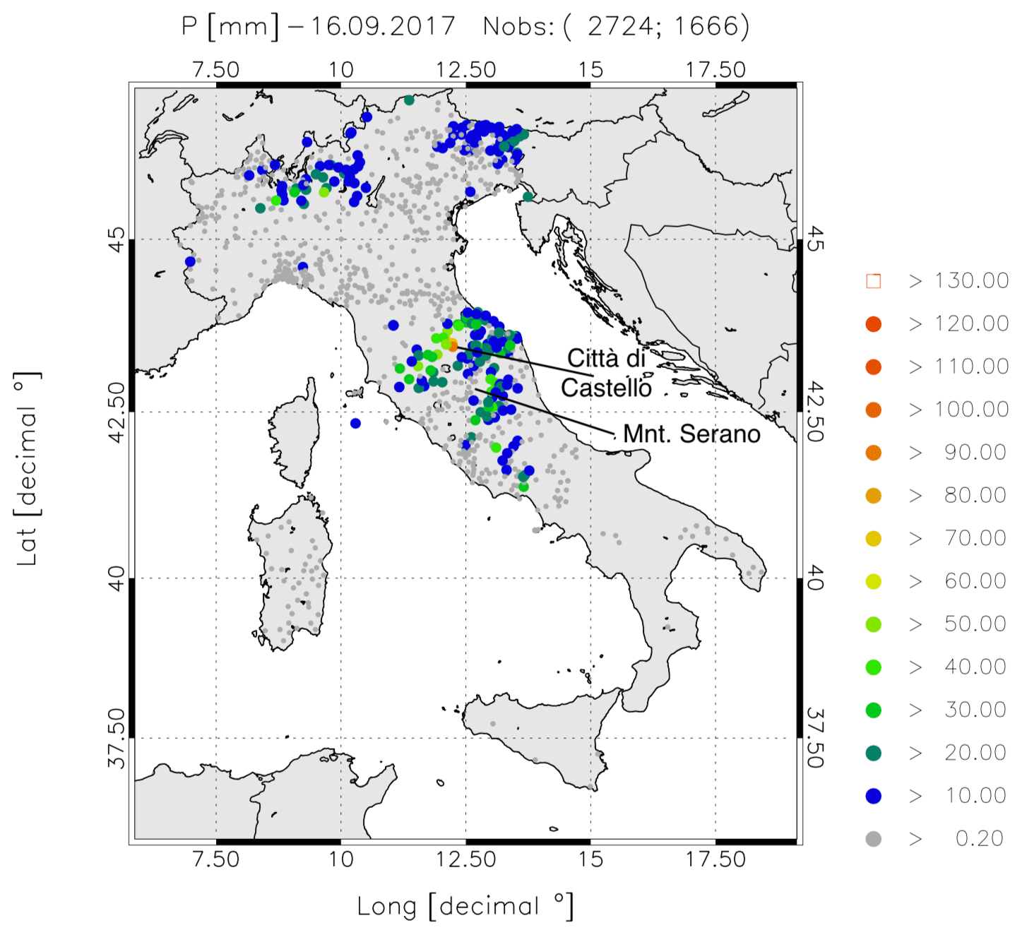
Figure 1Daily precipitation over Italy on 16 September 2017. Only rain gauges observing at least 0.2 mm d−1 are shown. The first number in the figure title within brackets represents the available rain gauges, while the second number represents rain gauges observing at least 0.2 mm d−1. The lowest precipitation class is represented by smaller dots, the largest by a red square. The locations of Città di Castello and Mount Serrano are indicated.
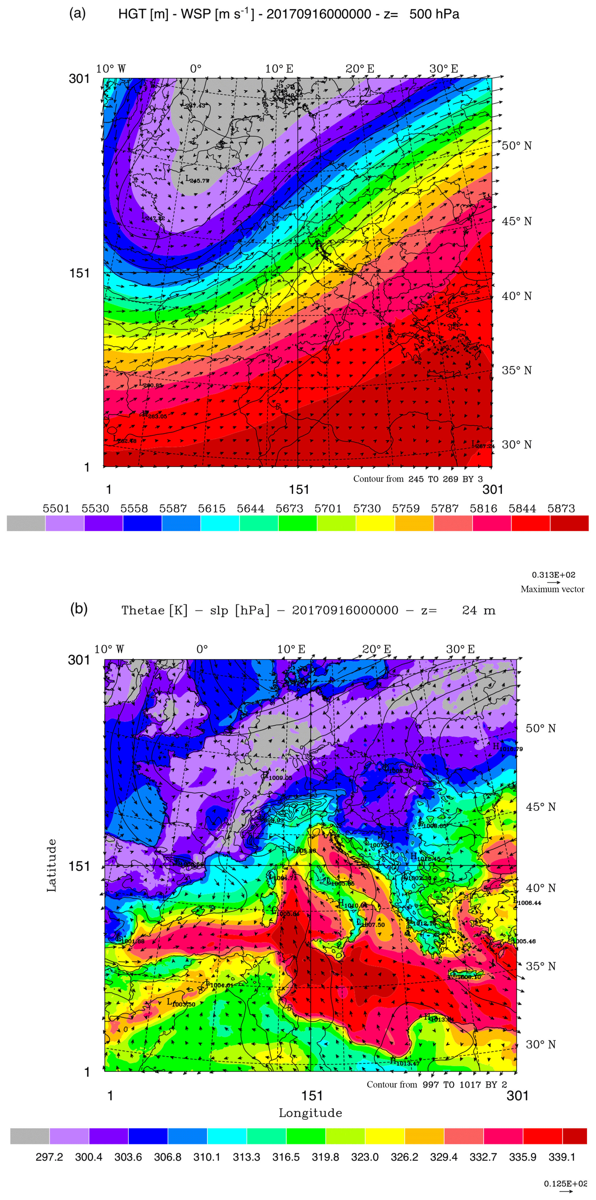
Figure 2(a) Geopotential height (filled contours), temperature (contours), and wind vectors at 500 hPa on 16 September 2017 at 00:00 UTC. Maximum velocity is 31 m s−1; (b) equivalent potential temperature (filled contours), sea-level pressure (contours), and wind vectors at 24 m above the surface (maximum value 13 m s−1). A low-pressure pattern forms over northern Italy, with a front in the western Mediterranean.
The synoptic conditions during the event are shown in Fig. 2. At 500 hPa (Fig. 2a), a trough, elongated in the SW–NE direction, extends over western Europe and air masses are advected from SW towards the western Alps. The interaction between the airflow and the Alps generates a low pressure to the lee of the Alps over northern Italy.
The analysis at the surface (Fig. 2b) shows the meteorological front represented by the equivalent potential temperature gradient between air masses advected over the Mediterranean Sea from the NW and air masses advected from the south over the Tyrrhenian Sea. The advection of warm unstable air masses towards central Italy is notable.
Infrared satellite images (Fig. 3), from 00:00 UTC on 16 September to 00:00 UTC on 17 September, show that the cold front structure moved slowly from NW to SE. Interestingly, at 00:00 UTC on 16 September, the well-defined cloud system over central Italy (red circle of Fig. 3a) that caused most of the daily precipitation observed between 43.50 and 45.0∘ N is apparent.
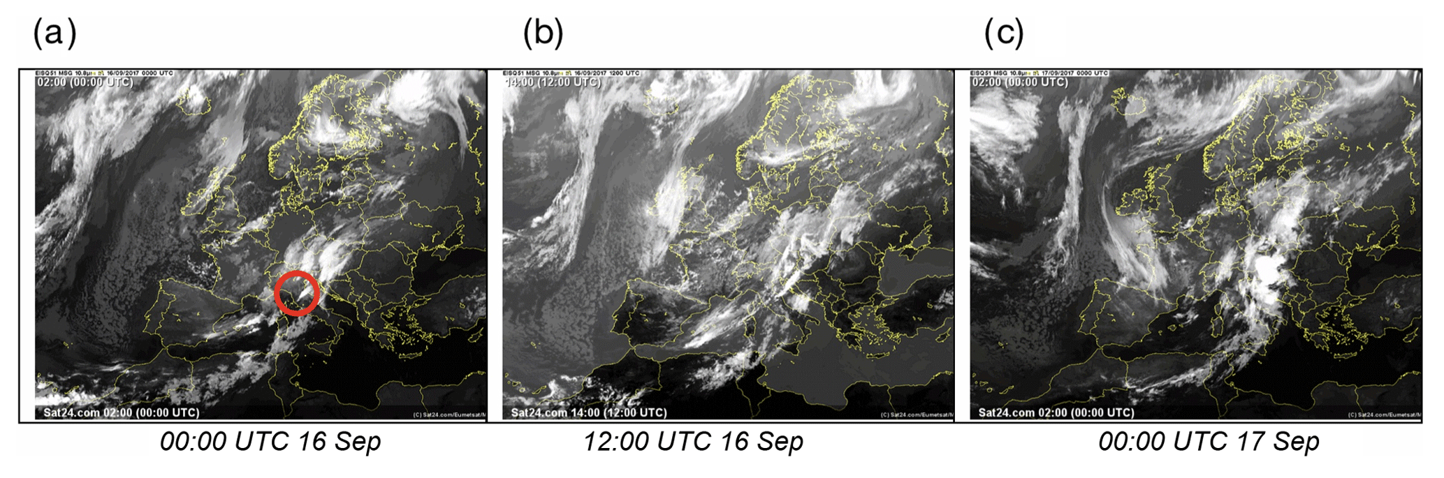
Figure 3(a) Satellite images (METEOSAT second generation) of the infrared channel, 10.8 µm, at 00:00 and 12:00 UTC on 16 September, and at 00:00 UTC on 17 September 2017. A well-defined cloud system is apparent inside the red circle of the image at 00:00 UTC on 16 September 2017. Source: https://www.sat24.com (last access: 8 August 2019); © EUMETSAT.
The well-defined cloud system over central Italy is also shown in the radar constant-altitude plan position indicator (CAPPI) at 3 km above sea level at 02:00 UTC on 16 September (Fig. 4). This CAPPI is formed by interpolating all the available data from the federated Italian radar network coordinated by the Department of Civil Protection (22 radars; see Sect. 3.3 for their positions) and it is also referred to as the national radar composite (hereafter also mosaic). Several convective cells exceeding 35 dBz can be noted over central-northern Italy. Importantly, the cloud system over central Italy shown by the satellite infrared channel at 00:00 UTC (Fig. 3a) and that of the radar at 02:00 UTC have similar positions, showing that the cloud system was active for several hours over central Italy.
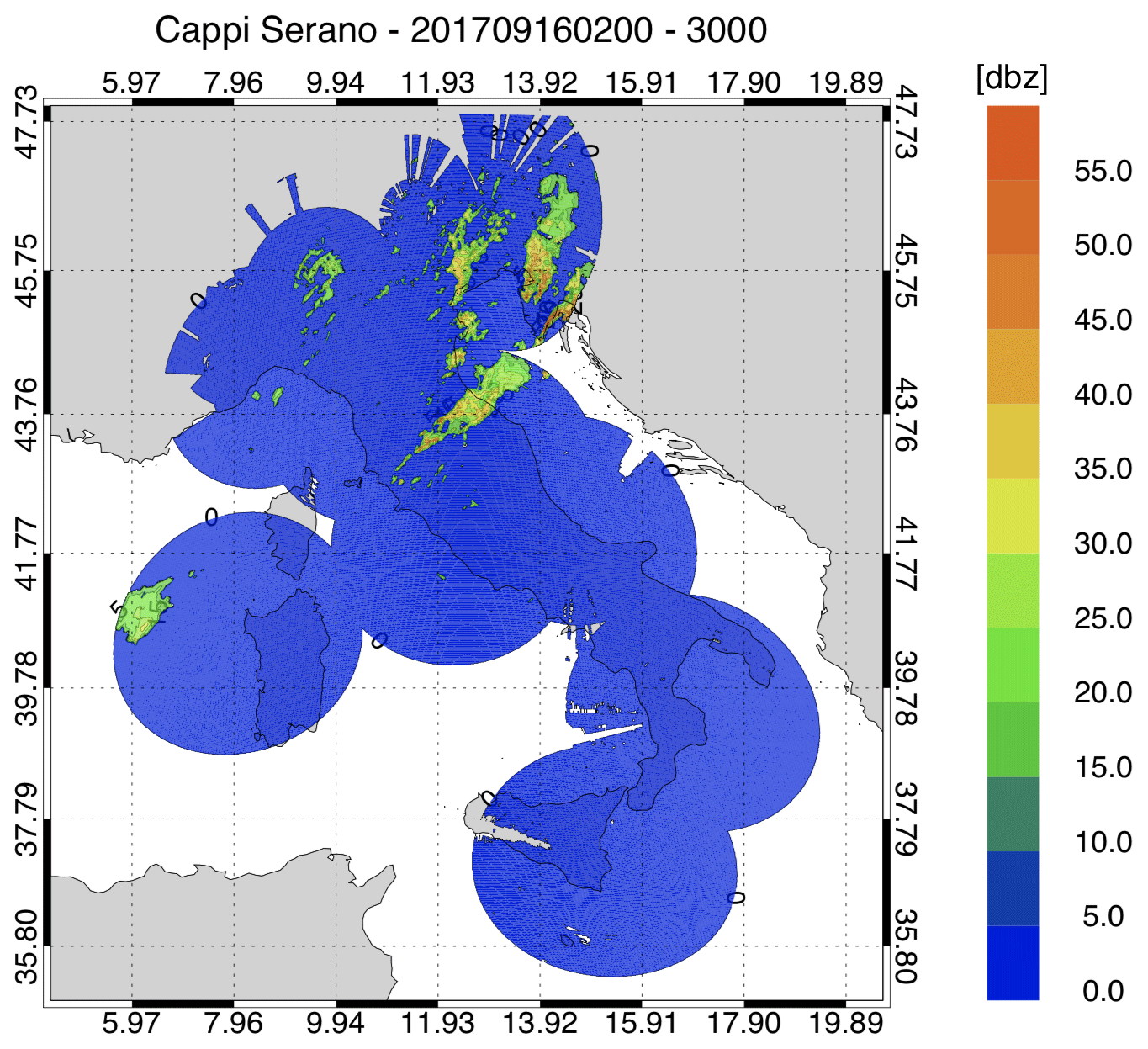
Figure 4National radar mosaic at 3 km above the sea level observed at 02:00 UTC on 16 September 2017.
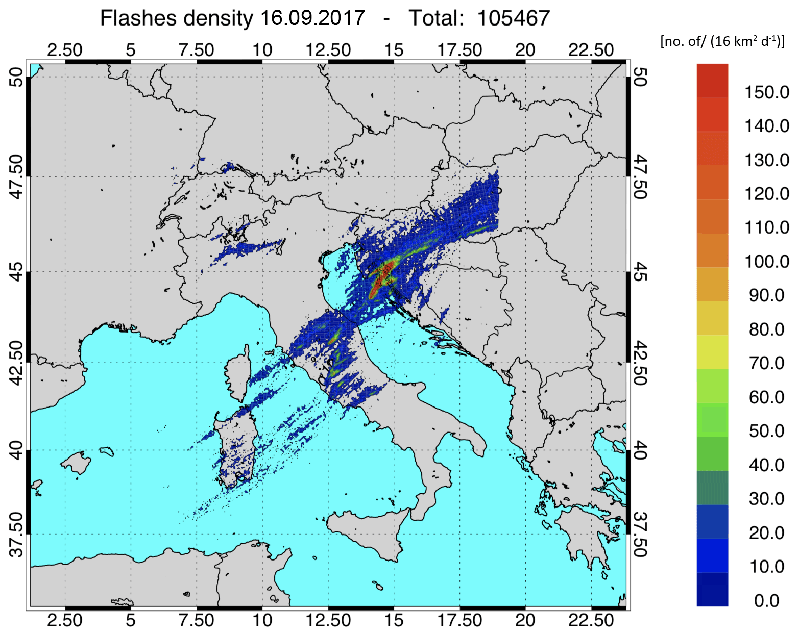
Figure 5Lightning density (number of lightning strikes per 16 km2 for the whole day) recorded on 16 September 2017. The total number of flashes is shown in the title.
Figure 5 shows the lightning recorded by LINET (lightning detection network; Betz et al., 2009) on 16 September 2017. More than 105 000 flashes were recorded; most of them occurred in the afternoon and evening, but a secondary maximum occurred in the night, from 00:00 to 06:00 UTC. In this phase, more than 3000 flashes were observed over central Italy.
2.2 The 9–10 September 2017 (Livorno) case study
On 9 and 10 September 2017, Italy was hit by a severe storm characterized by intense and widespread rainfall over the country. Figure 6a shows the precipitation on 9 September recorded by the Italian rain gauge network. Rainfall was intense over the Alps, where the maximum daily precipitation was observed (193 mm d−1), and over Liguria, with precipitation of the order of 30–50 mm d−1. One station over Tuscany reported 90 mm d−1, showing that intense precipitation had already started over the region. The storm on 9 September was intense: 20 rain gauges reported more than 100 mm d−1 and 70 rain gauges more than 60 mm d−1. In most cases, this precipitation occurred within a few hours.
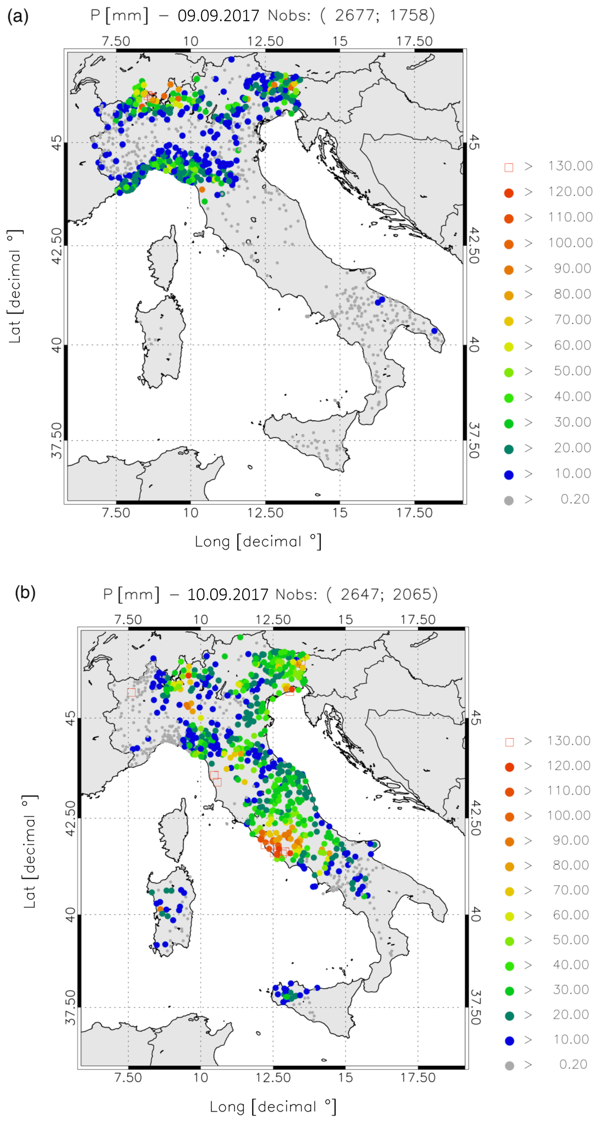
Figure 6(a) As in Fig. 1 but for (a) 9 September 2017 and (b) 10 September 2017.
The following day (see Fig. 6b) had higher rainfall. Precipitation occurred mainly over central Italy, especially over Lazio, and over northern Italy, in particular over the northeast. In Tuscany, the two stations close to the sea, in the Livorno area, recorded about 150 mm d−1 mostly falling between 00:00 and 06:00 UTC.
Synoptic conditions leading to this storm are shown in Fig. 7. At 500 hPa (Fig. 7a) a trough extended from northern Europe towards the Mediterranean. The interaction between the air masses and western Alps generated a low-pressure system to the lee of the Alps, which crossed the whole peninsula from NW to SE. It is noted that the divergent flow over central and northern Italy favoured upward motions.
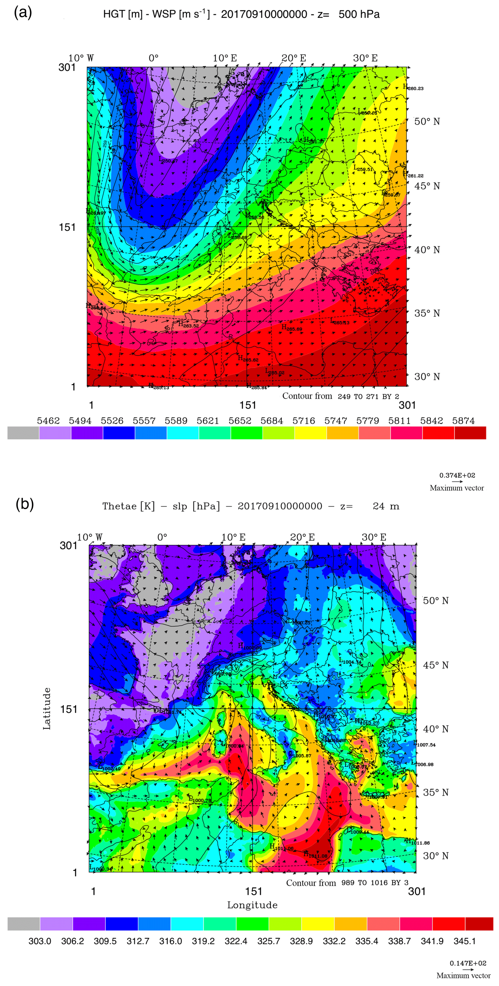
Figure 7(a) Geopotential height (filled contours), temperature (contours), and wind vectors at 500 hPa at 00:00 UTC on 10 September 2017. Maximum velocity is 37 m s−1; (b) equivalent potential temperature (filled contours), sea-level pressure (contours), and wind vectors at 24 m above the surface (maximum value 15 m s−1).
At the surface, Fig. 7b, the equivalent temperature gradient over the western Mediterranean is caused by the contrast between pre-existing air masses over the sea and air masses advected from France towards the Mediterranean. The pressure field at the surface advects air masses from the south over the Tyrrhenian Sea. These warm and humid air masses feed the cyclone during its development.
From a synoptic point of view, the Livorno and Serrano cases were similar and represented two cyclones developing to the lee of the Alps (Buzzi and Tibaldi, 1978). However, the Livorno case was more intense than Serrano.
The notable intensity of the Livorno case is confirmed by the lightning observations (Fig. 8). During the evening of 9 September (after 18:00 UTC) about 38 000 flashes were recorded by LINET. On 10 September about 290 000 flashes were recorded over Italy, following the movement of the storm from NW to SE. Therefore, more than 300 000 flashes were recorded from 18:00 UTC on 9 September to 00:00 UTC on 11 September, which is more than 3 times those recorded for Serrano.
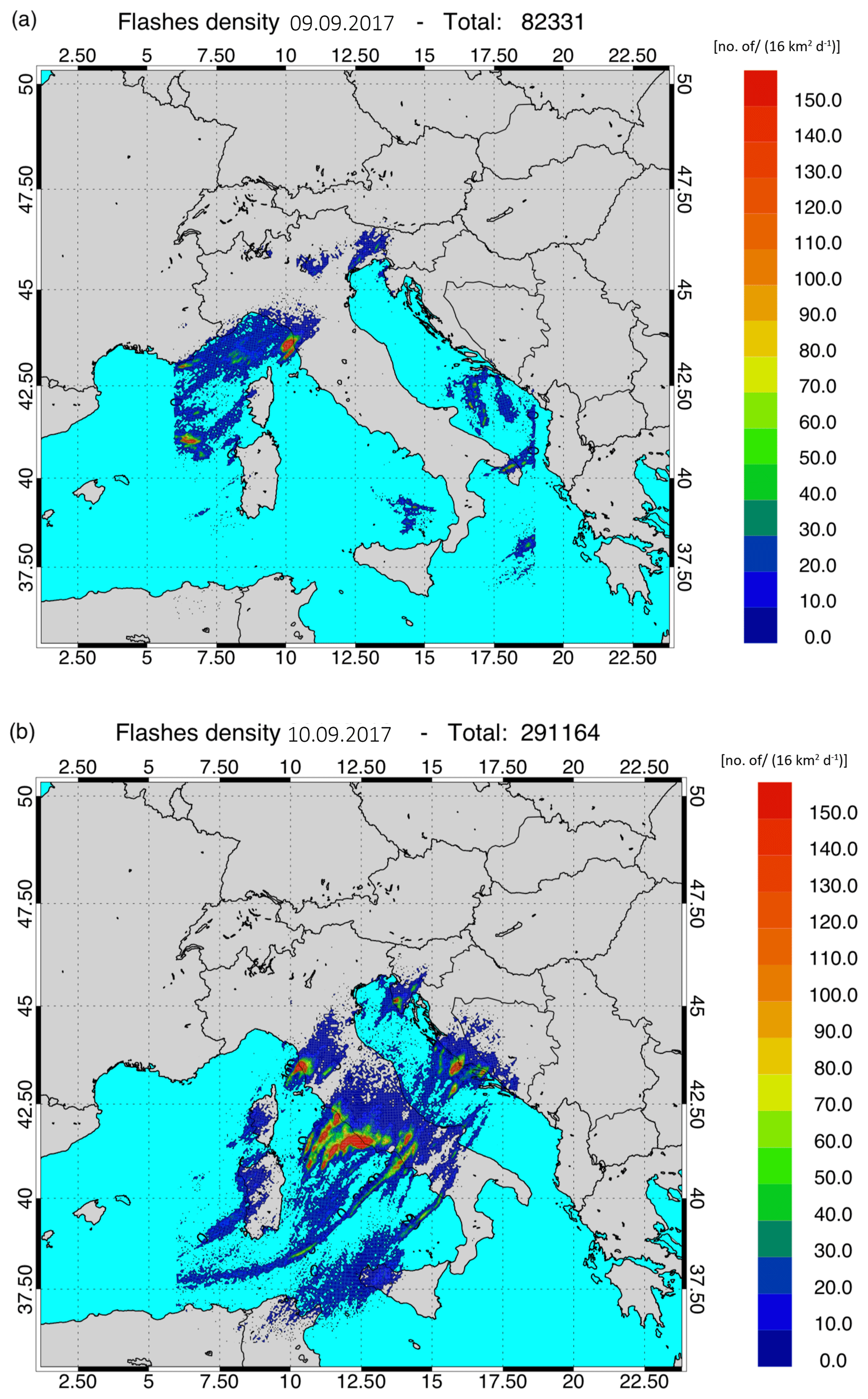
Figure 8(a) Lightning density (lightning number per 16 km2 for the whole day) recorded on 9 September 2017; (b) as in (a) for 10 September 2017. The number of flashes on each day is shown in the title.
Thermal infrared satellite images (channel, 10.8 µm; Fig. 9) show the extension of the cloud coverage every 12 h. It is very evident that the cloud system was associated with a cold front over Europe. More specifically, the satellite image at 00:00 UTC shows the cloud system over the Livorno area (red circle in Fig. 9b), before the most intense precipitation period over Tuscany (00:00–06:00 UTC), while Fig. 9c shows the cloud system over central Italy (orange circle), at the end of the period of intense precipitation over Lazio (06:00–12:00 UTC).
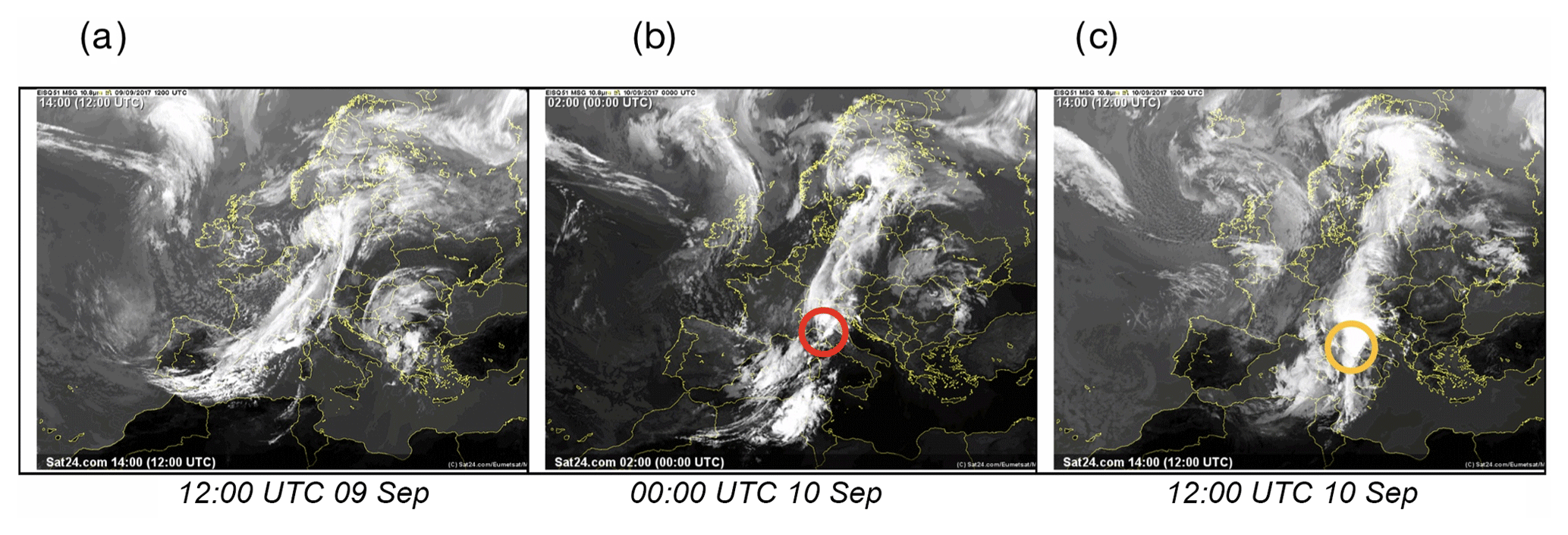
Figure 9(a) Satellite images (METEOSAT second generation) of the infrared channel, 10.8 µm, at 12:00 UTC on 9 September 2017, at 00:00 and 12:00 UTC on 10 September 2017. The red circle in Fig. 9b and the orange circle in Fig. 9c show the Livorno and Lazio areas, respectively. Source: https://www.sat24.com; © EUMETSAT.
We conclude the synoptic analysis of the case study with two CAPPIs at 3 km observed by the radar network of the Department of Civil Protection. The CAPPI in Fig. 10a, at 00:00 UTC on 10 September, shows the cloud system over Tuscany with reflectivity factors up to 40 dBz. Other clouds caused rainfall over northern Italy. The CAPPI of Fig. 10a is the last one assimilated by the 00:00–03:00 UTC VSF on 10 September described in detail in Sect. 4.2.1.
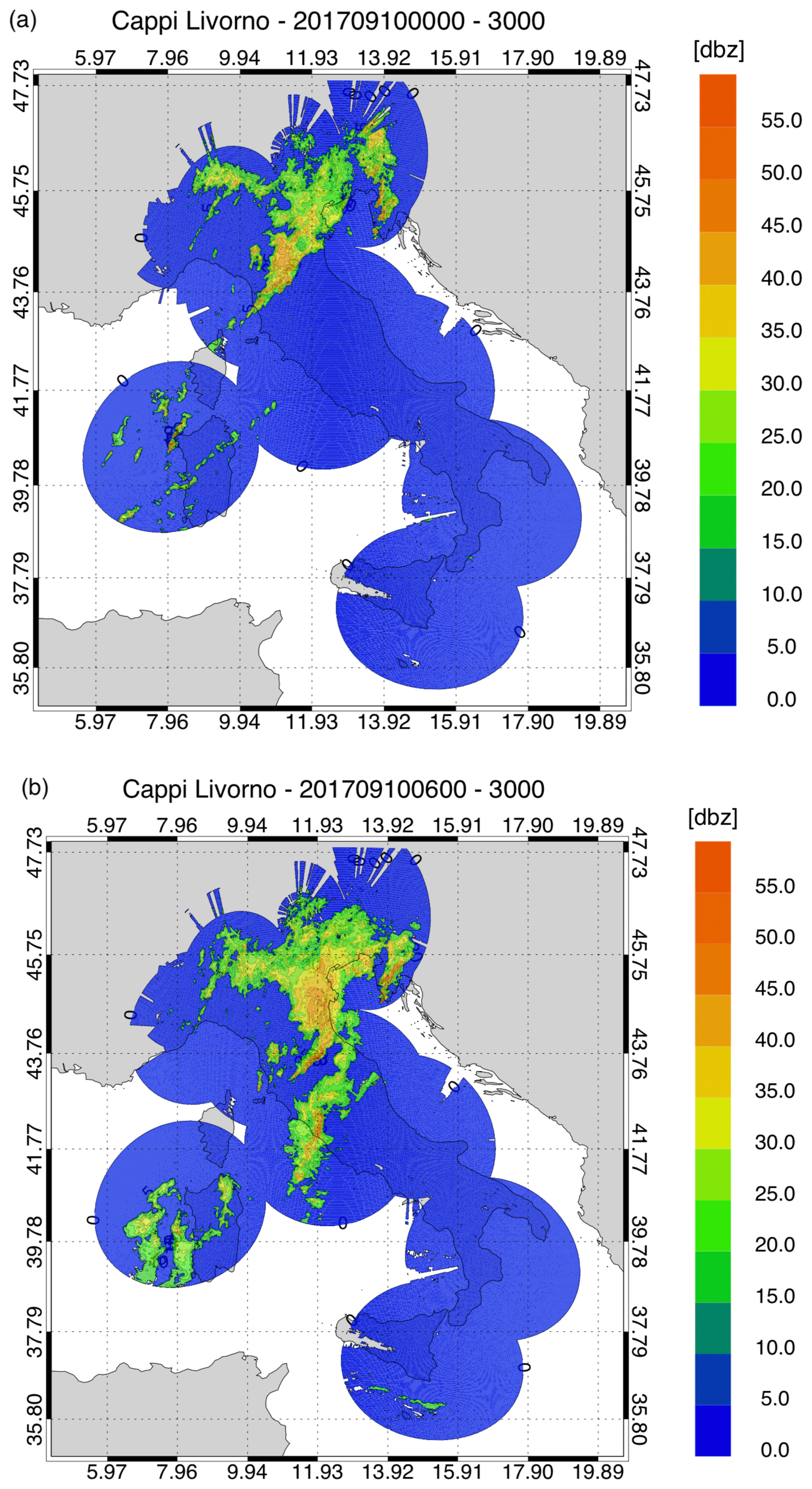
Figure 10(a) National radar mosaic at 3 km above the sea level observed at 00:00 UTC on 10 September 2017; (b) as in (a) at 06:00 UTC.
Figure 10b shows the CAPPI of the national radar mosaic at 3 km above the sea level and at 06:00 UTC. The cloud system is moving towards central Italy with reflectivity factors up to 45 dBz. Other cloud systems are apparent over northern Italy. Figure 10a–b represent the movement of the storm towards the SE well and Fig. 10b shows the last CAPPI assimilated by the 06:00–09:00 UTC VSF shown in Sect. 4.2.2.
3.1 RAMS@ISAC and simulations set-up
The RAMS@ISAC is used as a NWP driver in this work. The model is based on the RAMS 6.0 model (Cotton et al., 2003) with the addition of four main features, as well as a number of minor improvements. First, it implements additional single-moment microphysical schemes, whose performance is shown in Federico (2016): among them, the WSM6 (Hong and Lim, 2006) is used in this paper. Second, it predicts the occurrence of lightning following the diagnostic method of Dahl et al. (2011), with the implementation discussed in Federico et al. (2014). Third, the model assimilates lightning through nudging (Fierro et al., 2012, 2015; Federico et al., 2017a). Fourth, the model implements a 3D-Var data assimilation system (Federico, 2013, hereafter also RAMS-3DVar), whose extension to the radar reflectivity factor is presented in this paper (Sect. 3.3).
The list of the physical parameterization schemes used in the simulations of RAMS@ISAC is shown in Table 1.
Table 1RAMS@ISAC physical parameterizations used in this paper.

Considering the domains and the configuration of the grids (Fig. 11 and Table 2), two different set-ups are used for Serrano and Livorno. For the first case, we use the domains D1 and D2, while for Livorno we also use the domain D3. The first domain covers a large part of Europe and extends over North Africa. Grid horizontal resolution is 10 km (R10). The second domain covers all of Italy and part of Europe and the grid has 4 km horizontal resolution (R4). The third domain covers the Tuscany region, has 4∕3 km horizontal resolution (R1), and it is used for Livorno to represent the precipitation field over Tuscany with higher spatial detail. The fine structures of the precipitation field are smeared out over Tuscany using only domains D1 and D2. The operational implementation of the RAMS@ISAC model uses the domains D1 and D2 and no refinements for specific areas of Italy are used because this would require a computing power which is not currently available. Also, grid refinements over Italy would require careful testing of the model performance and data assimilation system, which are out of the scope of this paper.
Table 2Basic parameters of the RAMS@ISAC grids (R10, R4, and R1, corresponding, respectively, to the domains D1, D2, and D3). NNXP is the number of grid points in the WE direction, NNYP is the number of grid points in the NS direction, NNZP is the number of vertical levels, DX is the size of the grid spacing in the WE direction, and DY is the grid spacing in the SN direction. Lx, Ly, and Lz are the domain extensions in the NS, WE, and vertical directions. CENTLON and CENTLAT are the coordinates of the grid centres.
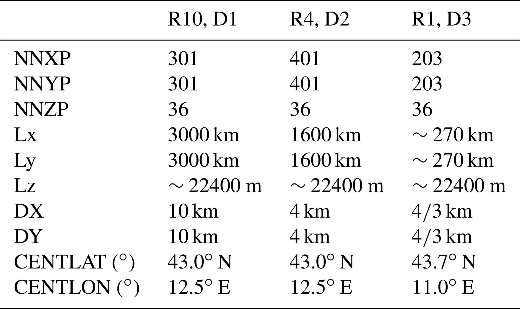
All domains share the same vertical grid, which covers the troposphere and the lower stratosphere. Vertical levels are more packed close to the ground. Among the 36 levels used in this paper 10 are below 1 km, 14 below 2 km, and 17 below 3 km. The first vertical level is at 50 m above the surface in the terrain following coordinates used by RAMS@ISAC; level 21 is at 5122 m. Above 6 km the model levels are about 1000 m apart, while the maximum allowed distance between two levels is 1200 m. The complete list of the vertical levels is shown in the Supplement of this paper (Table S2 in the Supplement).
The vertical grid is the same as the operational setting of RAMS@ISAC and is a compromise between vertical resolution and computing time. The number of vertical levels will be increased to 42, starting from September 2019, to better resolve the phenomena in this direction (planetary boundary layer processes, vertical motions, interaction between air masses and orography, etc.). Nevertheless the current setting was successfully applied to the forecast of several heavy precipitation events over Italy. A sensitivity test, using 42 vertical levels for the Livorno case, shows similar results to those reported in Sect. 4. Details on this simulation can be found in the Supplement of this paper.
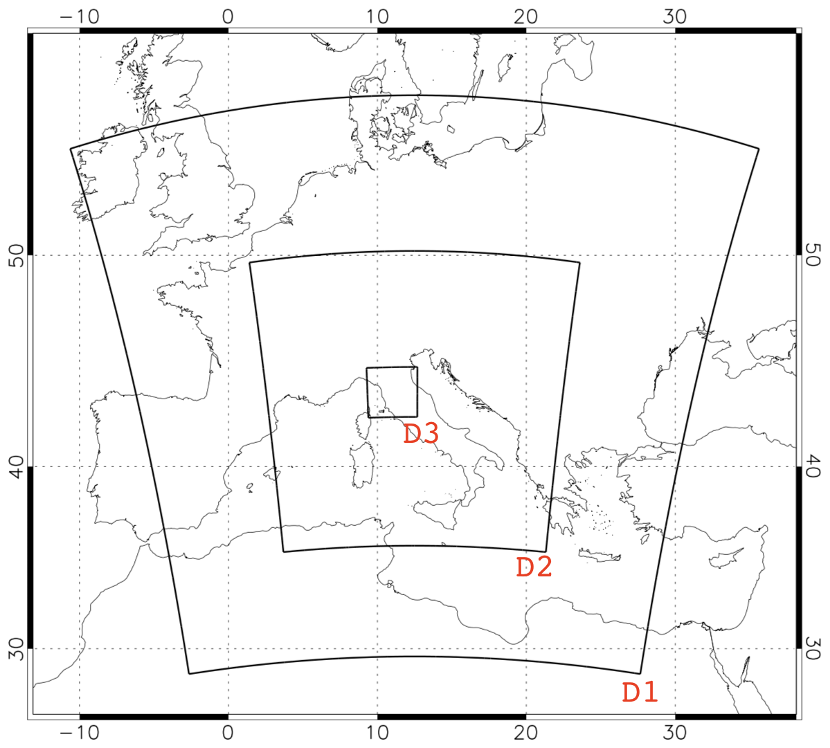
Figure 11The three domains used in RAMS@ISAC. The model grid over domain D1 has 301 grid points in the NS and WE directions and has 10 km horizontal resolution; the model grid over domain D2 has 401 grid points in the NS and WE directions and has 4 km horizontal resolution. The model grid over domain D3 has 203 grid points in the NS and WE directions and has 4∕3 km horizontal resolution. All grids have the same 36 vertical levels spanning the 0–22.4 km vertical layer.
The nesting between the first and second domains is one-way, while the nesting between the second and the third domains is two-way.
VSF was implemented as shown in Fig. 12. First a run with the R10 configuration was performed using the 0.25∘ horizontal resolution Global Forecast System (GFS) analysis–forecast cycle issued at 12:00 UTC as initial and boundary conditions. The R10 run, which started at 12:00 UTC on 16 September for Serrano and at 12:00 UTC on 9 September for Livorno, lasted 36 h and does not assimilate either radar reflectivity factor or lightning. The R10 run was not updated after the acquisition of new data by the analysis system and this is a limitation of the results shown in this paper. However, a sensitivity test for the Livorno case study showed that this limitation does not have a significant impact on the results presented in the next section. Details on this experiment can be found in the Supplement of this paper.
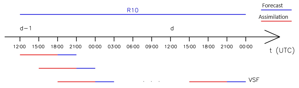
Starting from 12:00 UTC, 10 VSFs were performed using R4 for Serrano and both R4 and R1 for Livorno. The VSF lasted 9 h and used R10 simulation as initial and boundary conditions (one-way nesting). The 9 h forecast was divided into two parts: the first 6 h are the assimilation stage when RAMS@ISAC simulation was adjusted by data assimilation, whereas the last 3 h are the forecast stage, without data assimilation. During the assimilation stage, flashes are assimilated by nudging (Sect. 3.2), while radar reflectivity factor is assimilated every hour by RAMS-3DVar (Sect. 3.3).
It is noted that data assimilation is performed over the domain D2 (R4) only, and the innovations are transferred to the domain D3 (R1) for the Livorno case by the two-way nesting. The domain D3 is used for the Livorno case to refine the resolution of the precipitation field over Tuscany and to show the spatial and temporal precision of the precipitation forecast over Tuscany using data assimilation. However, its usage is exceptional because, as stated above, Italy is a complex orographic country and grid refinements for specific areas are used only after the occurrence of the event. For this reason, the domain D3 is usually not used in RAMS@ISAC and no statistics about the background error are available for this grid.
Because lightning and radar reflectivity factors are cloud-scale observations, their assimilation at higher horizontal resolution by 3D-Var is foreseeable in future works.
The verification of the VSF for precipitation was done by visual comparison of the model output with the rain gauge network of the Department of Civil Protection, which has more than 3000 rain gauges all over Italy.
In addition we considered the FBIAS (frequency bias; range [0, +∞)), where 1 is the perfect score, i.e. when no misses and false alarms occur), POD (probability of detection; range [0, 1], where 1 is the perfect score and 0 the worst value), ETS (equitable threat score; range [, 1], where 1 is the perfect score and 0 is a useless forecast), and TS (threat score; range [0, 1], where 1 is the perfect score and 0 the worst value). Scores were computed from 2×2 dichotomous contingency tables (Wilks, 2006) for different rainfall thresholds and for different neighbourhood radii. Moreover, performance diagrams (Roebber, 2009) were used to summarize the scores.
3.2 Lightning data assimilation
Lightning data are provided by LINET (lightning detection network; Betz et al., 2009; nowcast, 2019), which has more than 500 sensors worldwide with the greatest density over Europe (more than 200 sensors). The network has a good coverage over central Europe, and western Mediterranean (from 10∘ W to 35∘ E and from 30 to 60∘ N). The area of good coverage includes the region considered in this paper.
LINET exploits the VLF and LF (very low frequency and low frequency) electromagnetic bands and provides measurements of both intra-cloud (IC) and cloud-to-ground (CG) discharges. IC strokes are detected as long as lightning occurs within 120 km of the nearest sensor thanks to optimized hardware and advanced techniques of data processing (TOA-3D; Betz et al., 2004). According to Betz et al. (2009), LINET has a location accuracy of 125 m for an average distance of 200 km among the sensors verified by strikes into towers of known positions.
The good performance of the LINET network and its ability to detect IC strokes is shown in Lagouvardos et al. (2009) for a storm in southern Germany, while the good performance over Italy, including both CG and IC strokes, is discussed in Petracca et al. (2014).
The lightning data assimilation scheme is that of Fierro et al. (2012, 2014, 2015) and uses the total lightning, i.e. intra-cloud plus cloud-to-ground flashes.
The method starts by computing the water vapour mixing ratio qv:
where coefficients are set to A=0.86, B=0.15, C=0.30, D=0.25, and α=2.2, qs is the saturation mixing ratio at the model atmospheric temperature, and qg is the graupel mixing ratio (g kg−1). X is the number of total flashes (IC+CG) falling in a grid box of domain D2 (R4) in the past 5 min. The mixing ratio qv of Eq. (1) is computed only for grid points where flashes are recorded. More specifically, for each grid point we consider the number of flashes falling in a grid box centred at the grid point in the last 5 min. The mixing ratio of Eq. (1) is compared with that predicted by the model. If the mixing ratio of Eq. (1) is larger than the simulated one, the latter is nudged towards the value of Eq. (1), otherwise the modelled mixing ratio is left unchanged. This method can only add water vapour to the forecast.
The check and eventual substitution of the water vapour is performed every 5 min and it is made within the mixed phase layer zone (0 and −25 ∘C), wherein electrification processes caused by the collision of ice and graupel are the most active (Takahashi, 1978; Emersic and Sounders, 2010; Fierro et al., 2015).
The scheme of Fierro et al. (2012, 2015) was adapted to RAMS@ISAC in Federico et al. (2017a). In particular, the coefficient C of Eq. (1) was rescaled from that of Fierro et al. (2012) considering the different spatio-temporal resolution of gridded lightning data; then the coefficient C was tuned (increased) by sensitivity tests considering two case studies of HyMeX-SOP1 (15 and 27 October 2012; HyMeX stands for the Hydrological cycle in the Mediterranean Experiment – First Special Observing Period occurring between 6 September and 6 November 2012; Ducrocq et al., 2014). The C constant was adapted subjectively as a compromise of increasing the hits and minimizing false alarms. POD and ETS scores were considered metrics for this purpose. Then, Eq. (1) was applied to 20 case studies of HyMeX-SOP1 giving a statistically significant (90 %, or 95 % depending on the rainfall threshold) improvement of the RAMS@ISAC precipitation VSF (3 h).
Nevertheless, a definitive statistic on the performance of rainfall VSF to nudging formulation in RAMS@ISAC is missing and further studies are needed in this direction. Also, the optimal choice of the coefficients , and α is case dependent.
Fierro et al. (2012) applied the method using Earth Networks Total Lightning Network (ENTLN), which has a detection efficiency (DE) greater than 50 % for IC over Oklahoma, where the ENTLN data were used. The emphasis on IC flashes in the set-up of Fierro et al. (2012) is given because observational and model studies have provided evidence that IC flashes correlate better than CG flashes with various measures of intensifying convection (updraft strength, volume, graupel mass flux, etc.; MacGorman et al. 1989, 2005, 2011; Carey and Rutledge, 1998; Wiens et al., 2005; Kuhlman et al. 2006; Fierro et al., 2006; Deierling and Petersen, 2008). For these reasons methods using both IC and CG flashes perform better than those using CG only, CG flashes being correlated with the descent of reflectivity cores and the onset of the demise of the storm's updraft core (MacGorman and Nielsen, 1991).
The analysis of the case studies shows that IC strokes are about 30 % of the total number of strokes reported by LINET. Also, the fraction of IC strokes to the total strokes depends on the position. For example, for the Serrano case, the fraction of IC strokes detected by LINET over the area hit by the largest precipitation is more than 50 % while over the Adriatic Sea it decreases to 10 %.
It is also noted that the detection efficiency (DE) for IC strokes cannot be reliably compared between LINET and ENTLN because the area is different and the technical details about IC detection remain unclear (type of signals, VLF–LF or very high frequency (VHF), discrimination IC or CG).
For all the above reasons the application of the Fierro method to RAMS@ISAC is not straightforward and it is appropriate to study the dependence of the rainfall VSF on the nudging formulation. This subject is studied in the Supplement of this paper (Supplement Sect. S3) and the results show that the choice of the coefficient of Eq. (1) used in this paper is reasonable.
It is finally noted that despite the limitations noted above, the lightning data assimilation, with the setting of this paper, had a significant and positive impact on RAMS@ISAC rainfall VSF (Federico et al., 2017a, b).
3.3 Radar data assimilation
The method assimilates CAPPI of radar reflectivity factor operationally provided by the Italian Department of Civil Protection (DPC). Radar data are provided over a regular Cartesian grid with 1 km horizontal resolution and for three vertical levels (2, 3, 5 km above the sea level). The CAPPIs at 2, 3, and 5 km can be considered under-sampled vertical profiles. CAPPIs are composed starting from the 22 radars of the Italian Radar Network (Fig. 13), 19 operating at the C band (i.e. 5.6 GHz) and 3 at the X band (i.e. 9.37 GHz). The data quality control and CAPPI composition is performed by DPC. Data quality processing chain aims at identifying most of the uncertainty sources as clutter, partial beam blocking, and beam broadening. The radar observations are processed according to nine steps detailed in Vulpiani et al. (2014), Petracca et al. (2018), and references therein.
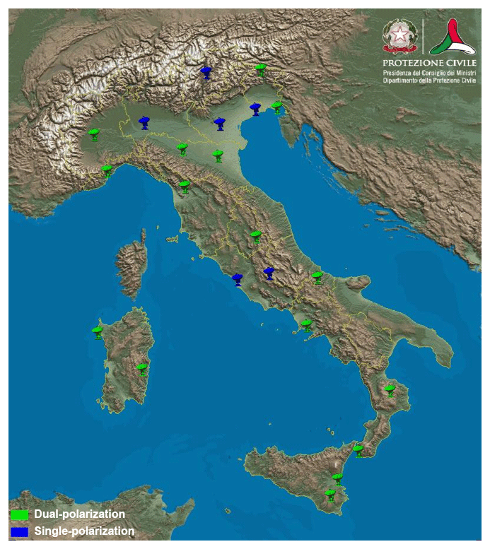
Figure 13The radar network of the Department of Civil Protection. Green radars operate with dual polarization; blue radars have single polarization.
Radial velocity is not assimilated into RAMS@ISAC because it is not operationally processed, and the scan strategy being optimized for quantitative precipitation estimation (QPE) purposes. Furthermore, the implementation of a radial velocity data assimilation scheme is under development in RAMS-3DVar and it is not currently available for testing. For these reasons, we did not consider the assimilation of this parameter.
Before entering data assimilation, the Cartesian grid is downscaled to 5 km by 5 km in order to reduce the numerical cost of the data assimilation and the effect of correlated observation errors (Rohn et al., 2001). Thus, the radar grid (Fig. 4, for example) is a Cartesian grid with 5 km grid spacing and three vertical levels.
It is important to note that pure sampling of the data could result in implementation of errors (for example reflectivity given by insects or birds) or extremes. Creating super-observations would reduce this problem, the main drawback being missing very localized phenomena. While the aim of this paper is to present the update of the data assimilation system of RAMS@ISAC and its application to two challenging cases, the problem of using super-observations will be considered in future studies because it impacts the results.
The methodology to assimilate radar reflectivity factor is that of Caumont et al. (2010), named 1D+3D-Var, which is a two-step process: first, using a Bayesian approach inspired by GPROF (Goddard profiling algorithm; Olson et al., 1996; Kummerow et al., 2001), 1-D pseudo-profiles of model variables are computed, and second those pseudo-profiles are assimilated by 3D-Var. Both steps are discussed below.
The first step computes a pseudo-profile of relative humidity, weighting the model profiles of relative humidity around the radar profile (Bayesian approach). The pseudo-profile is computed by
where RHi is the RAMS@ISAC vertical profile of relative humidity at a grid point inside a square of 50×50 km2 centred at the radar vertical profile, Wi is the weight of each profile, and is the relative humidity pseudo-profile. The weights are determined by the agreement between the simulated and observed reflectivity factors:
where hz is the forward observation operator, transforming the background column xi into the observed reflectivity factor. The radar forward observation operator is taken from the RIP (Read/Interpolate/Plot) software (https://dtcenter.org/wrf-nmm/users/OnLineTutorial/NMM/RIP/index.php, last access: 3 March 2019) and is given in the Supplement of this paper (Sect. S8). It assumes a Marshall–Palmer hydrometeor size distribution and Rayleigh scattering, and depends on the mixing ratios of rain, graupel, and snow.
The matrix Rz in Eq. (3) is diagonal and its value is nσ2, where σ is 1 dBz and n is the number of available observations in the vertical profile (from 1 to 3). In this way, we give more weight to vertical profiles containing more data.
The error of radar data is assumed to be small (1 dBz) for two reasons: (a) reflectivity data are carefully checked by the Civil Protection Department; (b) the performance of the control simulation, not assimilating any data, is rather poor for the case studies. This setting, however, could not be optimal for cases when the control forecast performs better. A sensitivity test using σ=5 dBz for the Livorno case showed small differences compared to σ=1 dBz. The results of this sensitivity test are detailed in the Supplement of this paper (Sect. S4).
It is important to point out that the 50 km length scale of the above step does not represent the horizontal correlation length scale of the background error, which determines the horizontal spread of the innovations in the 3D-Var data assimilation (the latter length scale is between 14 and 25 km depending on the level). The 50 km length scale is used to set a square for computing the pseudo-profile of relative humidity (Eq. 2). This profile is given by a weighted average whose weights are determined by the agreement between the simulated and observed reflectivity factors. The larger the agreement the larger the weight. This distance is appropriate because the spatial error of meteorological models in simulating meteorological features, for example fronts, can be of this order. The control simulation of the two events considered in this paper confirms this choice.
The method is not able to force convection when the model has no rain, snow, or graupel in a square around (50×50 km2) a radar profile with a reflectivity factor greater than zero. In this case, the pseudo-profile of relative humidity is assumed saturated above the lifting condensation level and with no data below (Caumont et al., 2010).
It is also noted that the method is able to reduce spurious convection when the reflectivity factor is simulated but not observed because the pseudo-profile of relative humidity gives more weight to the drier relative humidity profiles simulated by RAMS@ISAC inside the 50×50 km2 square centred at the radar profile. Of course, the ability to reduce spurious convection depends on the availability of dry model profiles around the specific radar profile (see the example below). Finally, if the observed profile is dry and the profile simulated by RAMS@ISAC is dry too, the pseudo-profile is not computed.
In summary, pseudo-profiles are computed for each profile of the radar grid whenever reflectivity is observed or simulated.
The pseudo-profiles computed with the procedure introduced above are then used as observations in the RAMS-3DVar data assimilation (Federico, 2013), minimizing the cost function:
where x is the state vector giving the analysis when J is minimized, xb is the background, B and R are the background and observation error matrices, is the pseudo-vertical-profile computed by Eq. (2), and h is the forward observation operator transforming the state vector (RAMS@ISAC water vapour mixing ratio) into observations. The cost function in RAMS-3DVar is implemented in incremental form (Courtier et al., 1994) and its minimization is performed by the conjugate-gradient method (Press et al., 1992). No multi-scale approach is used.
The background error matrix is divided into three components along the three spatial directions (). The Bx and By matrices account for the spatial correlation of the background error. The correlations are Gaussian with length scales between 14 and 25 km, depending on the vertical level. These distances are computed using the National Meteorological Center (NMC) method (Barker et al., 2012) applied to the HyMeX-SOP1 period. It is again stressed that the spread of the innovations along the horizontal spatial directions in the 3D-Var analysis is determined by the length scales of Bx and By matrices.
The Bz matrix contains the error for the water vapour mixing ratio, which is the control variable used in RAMS-3DVar. This error is about 2 g kg−1 at the surface and decreases with height. In particular, it is larger than 0.5 g kg−1 below 4 km, and less than 0.2 g kg−1 above 5 km. The vertical decorrelation of the background error depends on the level and can be roughly estimated to be 500–2000 m. The observation error matrix R in Eq. (4) is diagonal and observation errors are uncorrelated. This choice is partially justified due to the sampling of radar reflectivity factor observation by choosing one point every five grid points in both horizontal directions of the radar Cartesian grid. However, correlation observation errors have a significant impact on the final analysis, as shown for example in Stewart et al. (2013), and different choices of the matrix R will be considered in future studies.
The value of the elements on the diagonal of R depends on the vertical level and is one-fourth of the diagonal element of the Bz matrix at the corresponding height. With these settings, larger weights are given to the observations than to the background, and analyses strongly adjust the background towards observations. Bz matrix is computed using the NMC method (Parrish and Derber, 1992; Barker et al., 2004) applied to HyMeX-SOP1; this choice is motivated by the fact that HyMeX-SOP1 contains several heavy precipitation events over Italy and the background error matrix is representative of the convective environment of the cases considered in this paper. In particular, 10 out of 20 declared IOPs (intense observing periods) of HyMeX-SOP1 occurred in Italy (Ferretti et al., 2014). In contrast, the period of September 2017, especially before the events selected in this study, was characterized by fair and stable weather conditions over Italy and the background error matrix for September 2017 is less representative of the convective environment that characterizes the events of this paper.
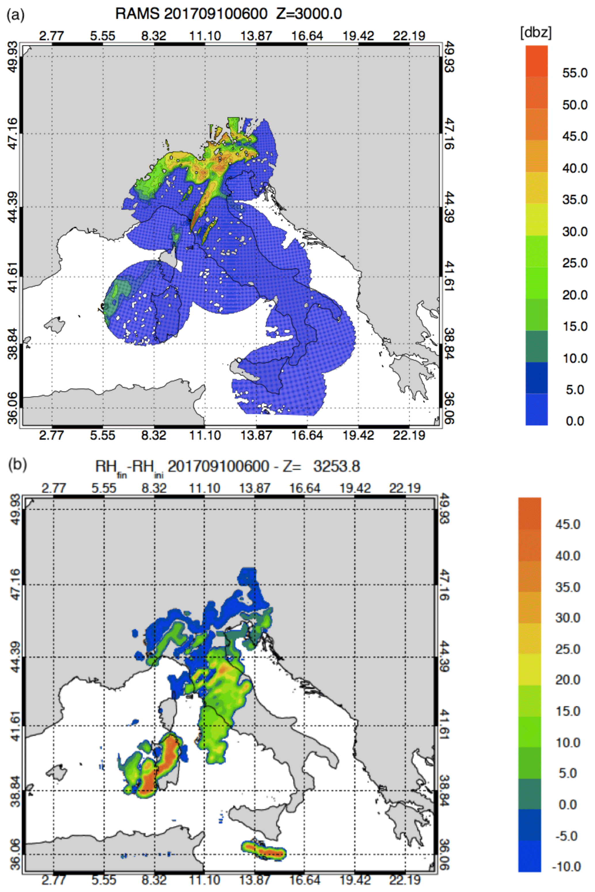
Figure 14(a) RAMS@ISAC reflectivity factor simulated 3 km above sea level at 06:00 UTC on 10 September 2017; (b) relative humidity difference between the analysis and the background at 06:00 UTC at the 3.2 km level in the terrain following the vertical coordinate of RAMS@ISAC.
Because it is the first time that we show the assimilation of radar reflectivity factor in RAMS@ISAC, it is useful to discuss an example of analysis. We select the analysis of the Livorno case study at 06:00 UTC. The observed CAPPI at 3 km above sea level is shown in Fig. 10b. The corresponding CAPPI simulated by the background is shown in Fig. 14a. In general, the comparison between simulated and observed reflectivity factor highlights the difficulty of the model to represent convection properly. In particular, the model is able to represent the convection over northern Italy but it has poor performance over Sardinia, south of Sicily, and over central Italy. The difference between the analysis and background relative humidity after and before the analysis is shown in Fig. 14b (absolute values less than 1 % are suppressed in the figure for clarity). Both positive (convection enhancing) and negative (convection suppressing) adjustments are found. Over central Italy, Sardinia, and south of Sicily relative humidity is increased because the model does not simulate the observed reflectivity (Fig. 10b). The occurrence of this condition added most of the water vapour to the RAMS@ISAC simulations for the case studies of this paper. Over northern Italy the model is partially dried for two different reasons: in the northwest of Italy because RAMS@ISAC simulates unobserved reflectivity, in the north and northeast of Italy because the model simulates larger values of reflectivity factor compared to the observations. The RAMS-3DVar reduces the relative humidity field north from Corsica island, where the RAMS@ISAC predicted unobserved reflectivity, while RAMS-3DVar did not suppress the unobserved convection west of Sardinia because the pseudo-profiles computed over this area were not appreciably drier than the background.
Cross correlations among different variables of the data assimilation system are neglected in this study and the application of RAMS-3DVar affects the water vapour mixing ratio only. Cross correlations among different variables can improve the performance of the data assimilation system, and an example of their impact in RAMS-3DVar is shown in Federico (2013). Nevertheless, the impact of cross correlations among different variables in the precipitation VSF will be explored in future works.
Since lightning data assimilation also adjusts the water vapour mixing ratio, it follows that the data assimilation presented in this study adjusts only this parameter.
Despite the fact that both radar reflectivity factor and lightning adjust the water vapour mixing ratio, different impacts on the VSF can be expected a priori because radar reflectivity factor and lightning are different types of observations and because they are used in different ways in the data assimilation system.
In particular, lightning is recorded when deep convection develops, while radar reflectivity factor is observed also for light stratiform rain. Flashes of ground-based networks, such as LINET, are available over the open sea, even if with a reduced detection efficiency, while radar reflectivity factor is confined to the range of coastal radars in the network. Lightning has a seasonal dependence over Italy, with the maximum in summer and autumn, while radar reflectivity factor is available in all seasons.
Also, differences in data assimilation of lightning and radar reflectivity factor play a role. In addition to the methods used to assimilate observations, lightning saturates the layer from 0 ∘C to −25 ∘C where and when it is detected, while radar reflectivity factor can be assimilated by pseudo-profiles or by saturation above the lifting condensation level where observed reflectivity is greater than zero.
Therefore, despite both observations adjusting the same model prognostic variable, which is a drawback of the methodology presented in this paper, the impacts of lightning and radar reflectivity factor is expected to be different as will be evident from the results of this paper.
There are, however, advantages using the methodology of this paper. In addition to being simple, it does not rely on approximate relationship between radar reflectivity factor and hydrometeor mixing ratio, leaving to the model the task of evolving the water vapour added and subtracted. Also, the impact of the data assimilation on model results is substantial (Fabry and Sun, 2010; Caumont et al., 2010), as also shown by the results of this paper.
Lightning and radar data assimilation may produce sharp gradients in the vertical direction caused by the addition of water vapour to specific layers. In the case of lightning, the water vapour is added by nudging to reduce sharp gradients. However, radar data assimilation, which accounts for the largest mass of water added to RAMS@ISAC (see Sect. S2), directly adjusts the water vapour into the model. Our experience with RAMS@ISAC, however, shows that results are reliable and the sudden addition of water vapour does not cause shocks to the model simulation, despite the notable gradients of specific humidity.
It is finally noted that the data assimilation increases or decreases the water vapour in the model depending on the cases. The eventual increase or decrease in the forecasted rainfall depends on the physical and dynamical processes occurring in the meteorological model, without any specific tuning.
In this section, we discuss the most intense phase of the Serrano case, 03:00–06:00 UTC on 16 September, and two VSFs forecasts, 00:00–03:00 UTC and 06:00–09:00 UTC on 10 September, for the Livorno case. The two VSF for Livorno correspond to the most intense phase of the storm in Livorno and to a very intense phase over the Lazio region, central Italy. The aim of the section is to show the notable improvement given by lightning and radar reflectivity factor data assimilation to the VSF.
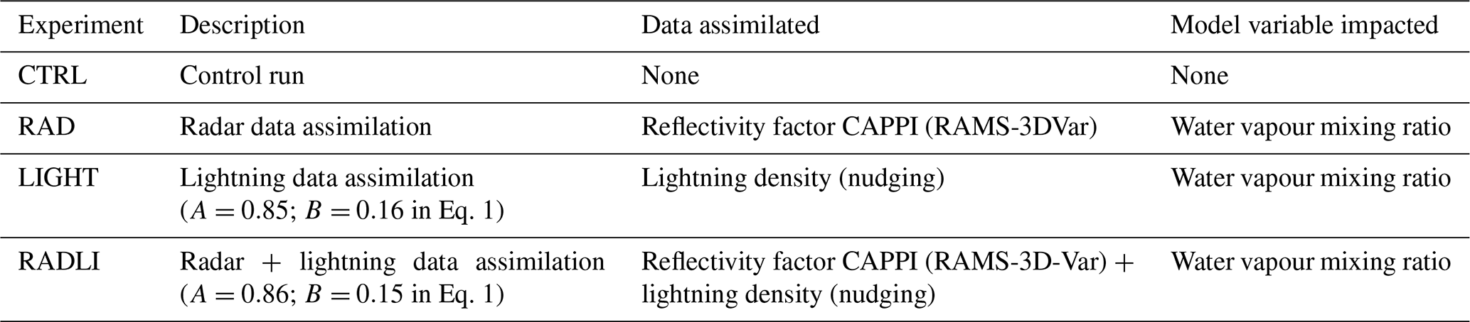
We consider four types of VSF (Table 3): (a) CTRL, without radar reflectivity factor or lightning data assimilation; (b) LIGHT, assimilating lightning but not radar reflectivity factor; (c) RAD, assimilating radar reflectivity factor but not lightning; and (d) RADLI, assimilating both lightning and radar reflectivity factor.
Several aspects of lightning and radar reflectivity factor data assimilation are considered in the Supplement of this paper: (a) the relative contribution to the total water mass given by lightning and radar reflectivity factor data assimilation (Sect. S2); (b) the sensitivity of the precipitation VSF to the nudging formulation (Sect. S3); (c) the sensitivity of rainfall VSF to two specific aspects of radar reflectivity factor data assimilation (Sect. S4); (d) the sensitivity of rainfall VSF to the RAMS@ISAC setting (Sect. S5); (e) the impact of lightning data assimilation for a case study well predicted by the control forecast (Sect. S6); (f) different plots of Figs. 15–17 (Sect. S7), and (g) the radar forward operator used in RAMS-3DVar (Sect. S8).
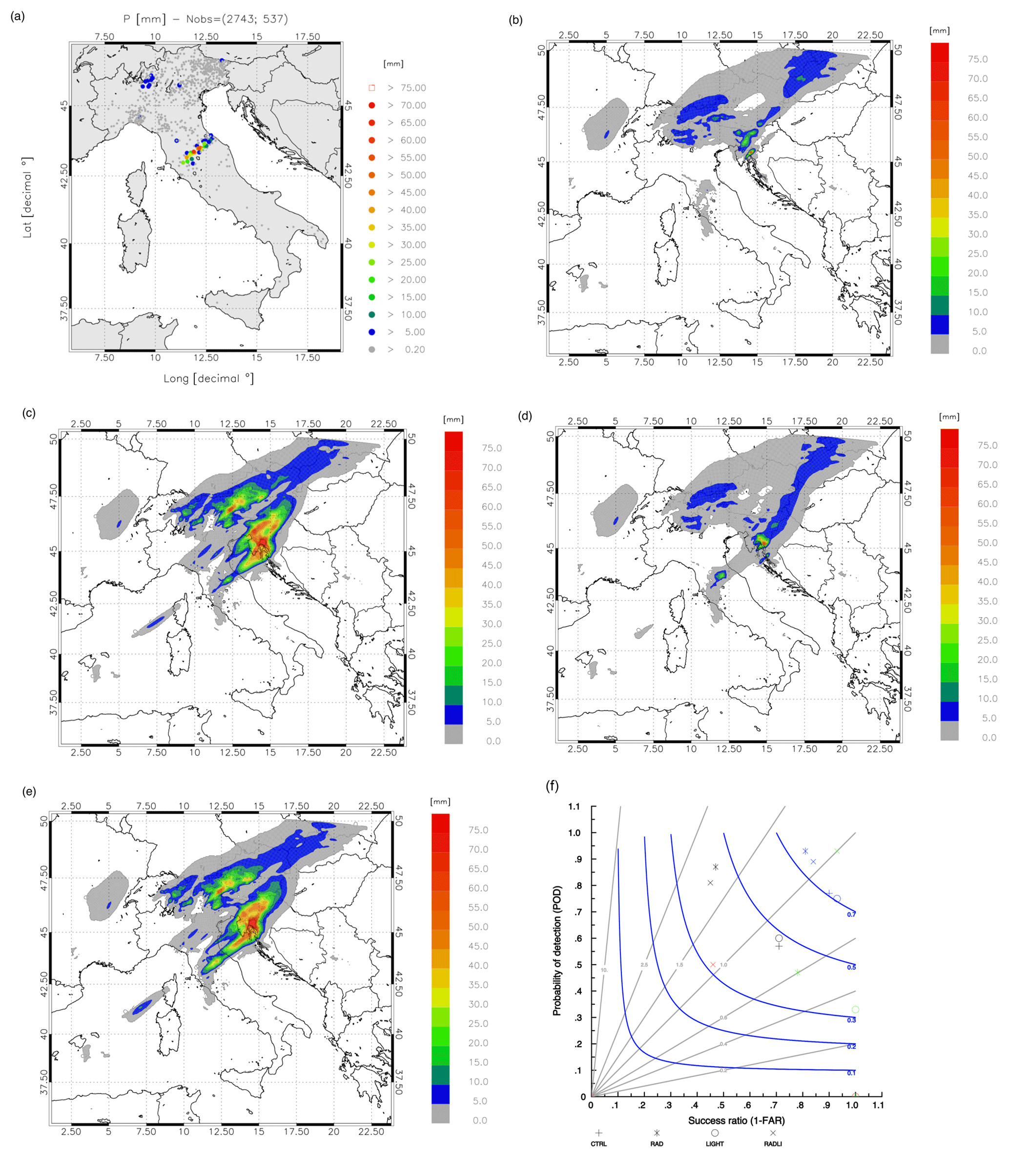
Figure 15(a) Rainfall reported by rain gauges between 03:00 and 06:00 UTC on 16 September 2017. Only rain gauges observing at least 0.2 mm every 3 h are shown. The first number in the title within brackets represents the available rain gauges, while the second number represents those observing at least 0.2 mm every 3 h; (b) rainfall VSF of CTRL for the same time interval as in (a); (c) as in (b) for RAD forecast; (d) as in (b) for LIGHT forecast; (e) as in (b) for RADLI forecast; (f) performance diagram: black symbols are for the nearest neighbourhood and for the 1 mm every 3 h threshold; red symbols are for the nearest neighbourhood and for the 30 mm every 3 h threshold; blue symbols are for the 25 km neighbourhood radii and for the 1 mm every 3 h threshold; green symbols are for the 25 km neighbourhood radii and for the 30 mm every 3 h threshold.
4.1 Serrano: 03:00–06:00 UTC on 16 September 2017
In this period, an intense and localized storm hit central Italy, while light precipitation occurred over northern Italy (Fig. 15a). Considering the storm over central Italy, 10 rain gauges observed more than 30 mm every 3 h, six more than 40 mm every 3 h, three more than 50 mm every 3 h, and one more than 60 mm every 3 h, the maximum observed value being 63 mm every 3 h.
The CTRL forecast, Fig. 15b, misses the rainfall over central Italy and considerably underestimates the precipitation area over northern Italy, giving unsatisfactory results.
The assimilation of the radar reflectivity factor improves the forecast, as shown in Fig. 15c. In particular, RAD forecast shows localized precipitation (30–35 mm every 3 h) close to the area were the most abundant precipitation was observed. Maximum precipitation is underestimated. Also, the RAD forecast better represents the precipitation over northern Italy compared to CTRL.
The rainfall forecast of LIGHT, Fig. 15d, shows some improvements compared to CTRL because the precipitation over central Italy has a maximum of 25–30 mm every 3 h, close to the area where the maximum precipitation was observed. LIGHT; however, it has a worse performance compared to RAD because it underestimates the precipitation area over northern Italy. LIGHT underestimates the maximum precipitation in central Italy.
The RADLI forecast, Fig. 15e, has the best performance. The precipitation over central Italy is well represented because the maximum rainfall (40–45 mm every 3 h) is in reasonable agreement with observations, and also because the area of intense precipitation (> 25 mm every 3 h) is elongated in the SW–NE direction in agreement with rain gauge observations. The precipitation over northern Italy is well represented by RADLI.
A performance diagram for 1 mm every 3 h and 30 mm every 3 h and for 4 and 25 km neighbourhood radii is shown in Fig. 15f. Different radii are considered to account for the well-known double penalty error (Mass et al., 2002; Mittermaier et al., 2013) caused by displacement errors of the detailed precipitation forecast in convection-allowing grids. RADLI has the best performance thanks to the synergistic contribution of lightning and radar reflectivity factor data assimilation.
4.2 Livorno
The Livorno case study lasted for several hours starting at 18:00 UTC on 9 September 2017 and ending more than a day later. The most intense phase in Livorno and its surroundings was observed during the night between 9 and 10 September. In the following, we will show two representative VSFs (3 h), including the most intense phase in Livorno.
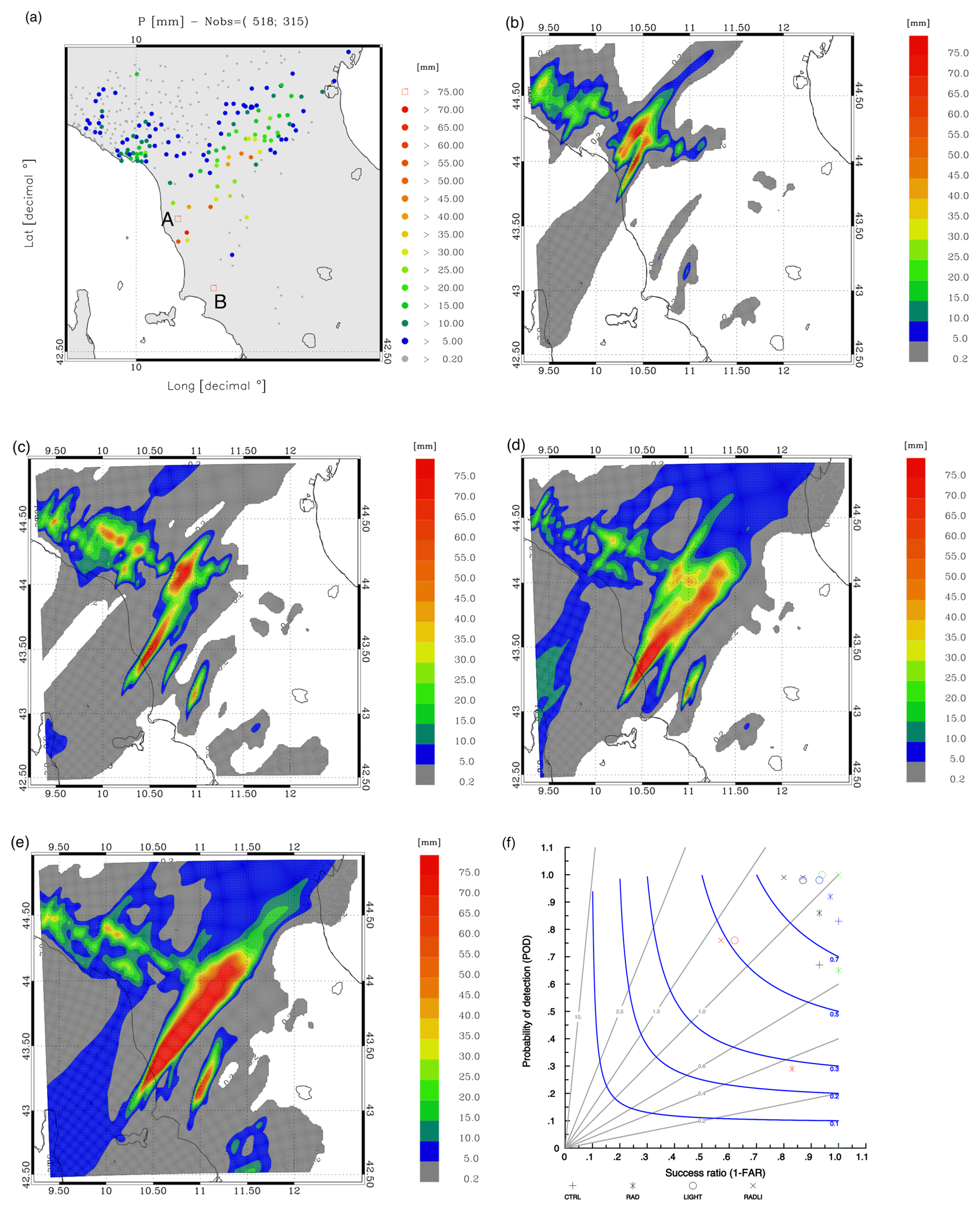
Figure 16(a) Rainfall reported by rain gauges between 00:00 and 03:00 UTC on 10 September 2017. Only stations reporting at least 0.2 mm every 3 h are shown. The first number in the title within brackets represents the number of rain gauges available over the domain, while the second number shows those observing at least 0.2 mm every 3 h; (b) rainfall VSF of CTRL for the same time interval as in (a); (c) as in (b) for the RAD forecast; (d) as in (b) for the LIGHT forecast; (e) as in (b) for the RADLI forecast. Labels A and B help to identify the positions of two rainfall maxima discussed in the text; (f) performance diagram: black symbols are for the nearest neighbourhood and for the 1 mm every 3 h threshold; red symbols are for the nearest neighbourhood and for the 30 mm every 3 h threshold; blue symbols are for the 25 km neighbourhood radii and for the 1 mm every 3 h threshold; green symbols are for the 25 km neighbourhood radii and for the 30 mm every 3 h threshold.
4.2.1 Livorno: 00:00–03:00 UTC on 10 September 2017
This period represents the most intense phase of the storm in Livorno. In particular, the rain gauge close to the label A (Fig. 16a) reported 151 mm every 3 h (Collesalvetti), while the one close to the label B measured 82 mm every 3 h. Among the 518 rain gauges reporting valid data, 75 observed more than 10 mm every 3 h, 31 more than 20 mm every 3 h, 17 more than 30 mm every 3 h, 9 more than 40 mm every 3 h, and 6 more than 50 mm every 3 h.
The CTRL precipitation forecast is shown in Fig. 16b. The forecast is poor because it misses the precipitation swath from the coast towards NE. A precipitation swath is forecasted about 50 km to the north of the real occurrence, but it is less wide compared to the observations.
The RAD forecast, Fig. 16c, shows that the assimilation of radar reflectivity factor gives a clear improvement of the forecast. The largest precipitation in the coastal part of the swath (we searched for the maximum in the area with longitudes between 10.20 and 10.70∘ E and latitudes between 43.10 and 43.60∘ N) is 94 mm every 3 h. Another local maximum is in the southern part of the domain (label B of Fig. 16a). The location of this maximum is well represented, but the forecasted value (55 mm every 3 h) underestimated the observed maximum (82 mm every 3 h).
An improvement, compared to both CTRL and RAD, is given by the assimilation of lightning (Fig. 16d). The maximum value close to Livorno, i.e. in the coastal part of the swath, is 158 mm every 3 h.
The LIGHT simulation shows the local maximum in the southern part of the domain (about 50 mm every 3 h), but the amount is underestimated.
Figure 16e shows the RADLI rainfall forecast. The precipitation swath from coastal Tuscany towards the NE is more intense compared to LIGHT and RAD. The maximum rainfall accumulated close to Livorno is 186 mm every 3 h. Also, the second precipitation maximum in the southern part of the domain reaches 70 mm every 3 h in good agreement with observations (82 mm every 3 h). RADLI is the only run giving a satisfactory precipitation VSF over southeastern Emilia Romagna (northeastern part of the domain), to the lee of the Apennines. It is also noted that the main precipitation swath forecasted by RADLI is too broad in the direction crossing the swath compared to the observations. This is confirmed by the FBIAS of RADLI (not shown), which is more than 3 for thresholds larger than 42 mm every 3 h.
The performance diagram (Fig. 16f) shows that LIGHT has better scores than RAD for this VSF.
4.2.2 Livorno: 06:00–09:00 UTC on 10 September 2017
In this period, the most intense precipitation occurred over the coastal part of Lazio (Fig. 17a). In more detail, among the 2695 rain gauges reporting valid data over the domain of Fig. 17a, 307 reported more than 10 mm every 3 h, 132 more than 20 mm every 3 h, 86 more than 30 mm every 3 h, 66 more than 40 mm every 3 h, 49 more than 50 mm every 3 h, and 35 more than 60 mm every 3 h. Among the 35 rain gauges measuring more than 60 mm every 3 h, 33 were over Lazio, showing the heavy rainfall that occurred over the region.

Figure 17(a) Rainfall reported by rain gauges between 06:00 and 09:00 UTC on 10 September 2017. For this time period 2695 rain gauges reported valid observations in the domain. However only stations reporting at least 0.2 mm every 3 h are shown The first number in the title within brackets represents the number of rain gauges available over the domain, while the second number shows those observing at least 0.2 mm every 3 h; (b) rainfall VSF of CTRL in the same time interval as (a); (c) as in (b) for the RAD forecast; (d) as in (b) for the LIGHT forecast; (e) as in (b) for the RADLI forecast; (f) performance diagram: black symbols are for the nearest neighbourhood and for the 1 mm every 3 h threshold; red symbols are for the nearest neighbourhood and for the 30 mm every 3 h threshold; blue symbols are for 25 km neighbourhood radii and for the 1 mm every 3 h threshold; green symbols are for 25 km neighbourhood radii and for the 30 mm every 3 h threshold.
Some precipitation persisted over Tuscany but the rainfall is much lower compared to the previous 6 h (the rainfall over Tuscany between 03:00 and 06:00 UTC was very intense, not shown).
Figure 17b shows the rainfall simulated by CTRL. The forecast is unsatisfactory, mainly for the following two reasons: (a) heavy precipitation is simulated over Tuscany (> 75 mm every 3 h), also close to the Livorno area; (b) precipitation is missed over central Italy. The rainfall over the NE of Italy is well represented in space, but overestimated.
Considering the evolution of the CTRL forecast for the two VSFs of Livorno, we conclude that it was able to predict abundant rain over Livorno, but the rainfall forecast was delayed compared to the real occurrence. A similar behaviour was found in Ricciardelli et al. (2018) using the WRF model, showing that the results of this paper for Livorno are likely not tied to the specific model used.
The rainfall simulated by RAD (Fig. 17c) clearly improves the forecast compared to CTRL. First, the precipitation over Lazio is well predicted. Second, the precipitation over Tuscany is less than for CTRL, showing the ability of radar reflectivity factor data assimilation to dry the model when it predicts reflectivity that is not observed. It is noted, however, that the area of intense rainfall (> 60 mm every 3 h) is overestimated by RAD, which has a wet forecast. The wet bias of the RAD forecast is apparent in the representation of the rainfall VSF shown in the Supplement of this paper (Fig. S12).
The LIGHT forecast, Fig. 17d, shows a worse performance compared to RAD for this time period. The precipitation forecast is mainly over Tuscany, where it is overestimated, with a small precipitation spot over Lazio.
The precipitation forecast of RADLI, Fig. 17e, represents the precipitation over Lazio very well, and the rainfall amount is better predicted compared to RAD. The precipitation over Sardinia is well represented by RADLI as well as the precipitation over the central Alps, giving the best results among all VSFs.
Figure 17f shows the better performance of RAD compared to LIGHT for this precipitation VSF. RADLI has the best performance and is closer to the upper right corner of the diagram.
To better understand the changes of the precipitation VSF for different data assimilation set-ups, Fig. 18 shows maps of water vapour mixing ratio averaged between 3 and 10 km at the end of the assimilation phase (06:00 UTC on 10 September 2017). It is important to note that those maps contain the effects of both data assimilation and model evolution.
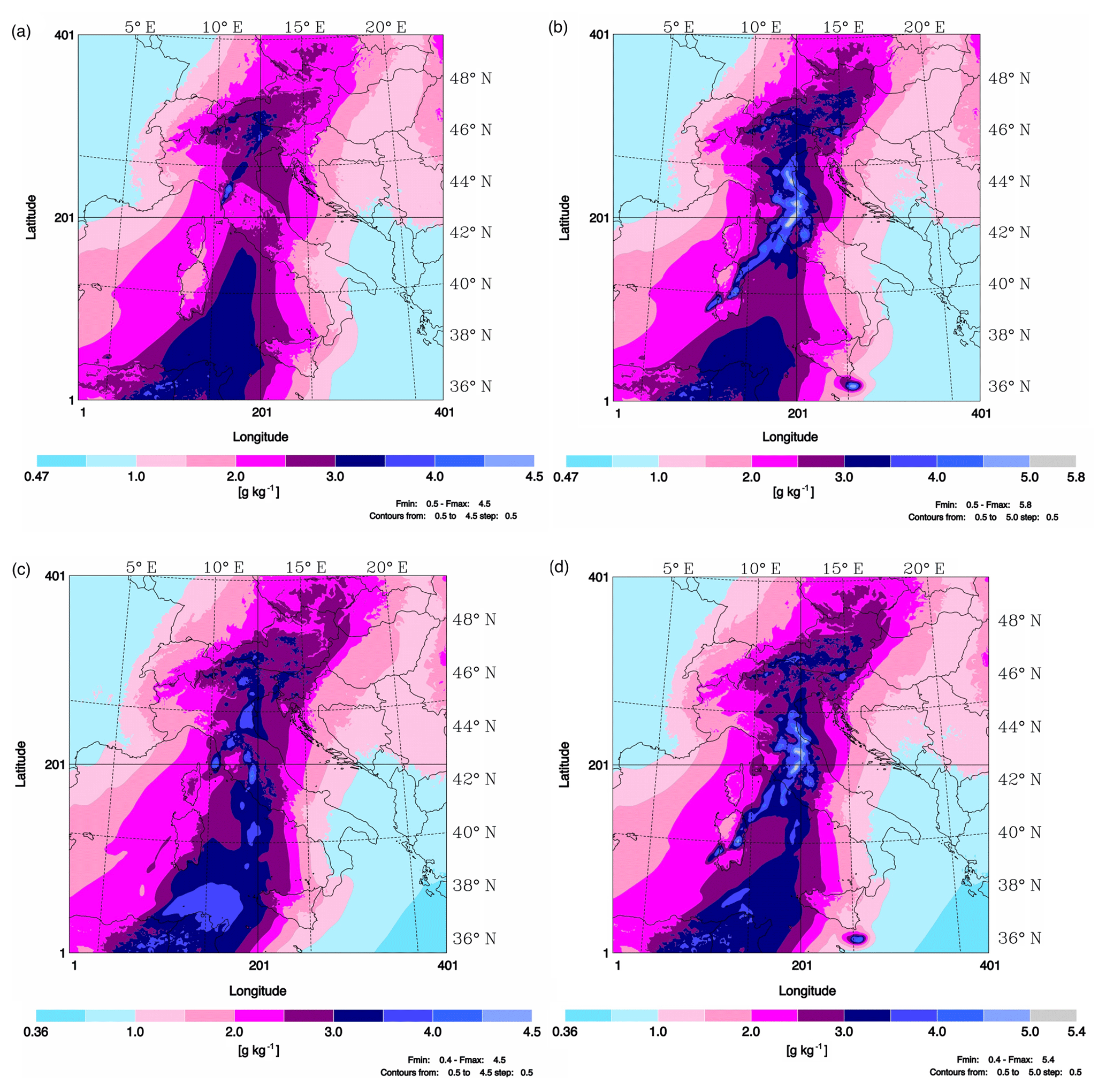
Figure 18Water vapour mixing ratio averaged between 3 and 10 km at 06:00 UTC on 10 September 2017 for (a) CTRL, (b) RAD, (c) LIGHT, and (d) RADLI.
The comparison between CTRL (Fig. 18a) and RAD (Fig. 18b) shows that RAD has a line of high water vapour values over central Italy, extending over the Tyrrhenian Sea and Sardinia, which is not simulated by CTRL. This line results from both radar data assimilation and convection, which transports water vapour from lower to upper levels. The comparison between CTRL and RAD shows the substantial impact of radar reflectivity factor data assimilation on the model evolution despite not using the relationship between hydrometeor mixing ratios and radar reflectivity factor in data assimilation.
LIGHT averaged water vapour (Fig. 18c) over the Tyrrhenian Sea and west of Sicily is higher compared to CTRL because of lightning data assimilation and model processes. Convection develops over Tuscany, northern Lazio, and NE of Italy, causing the increase in averaged water vapour in those areas.
Because RAD and LIGHT both assimilate water vapour it is important to highlight the differences between the two fields. First, LIGHT it is not able to represent a compact line of high water vapour over central Italy that, in the following hours, caused high precipitation over Lazio. Second, averaged water vapour simulated by RAD is larger than for LIGHT over central Italy, which is caused by deeper convection developing in RAD than in LIGHT, as well as by the different contributions of data assimilation. Finally, RADLI (Fig. 18d) is similar to RAD but it also shares features with LIGHT such as the increase in water vapour over the Tyrrhenian Sea.
It is also interesting to compare vertical cross sections of relative humidity for different data assimilation set-ups. Figure 19 show the longitude-height cross sections of relative humidity from different data assimilation configurations.
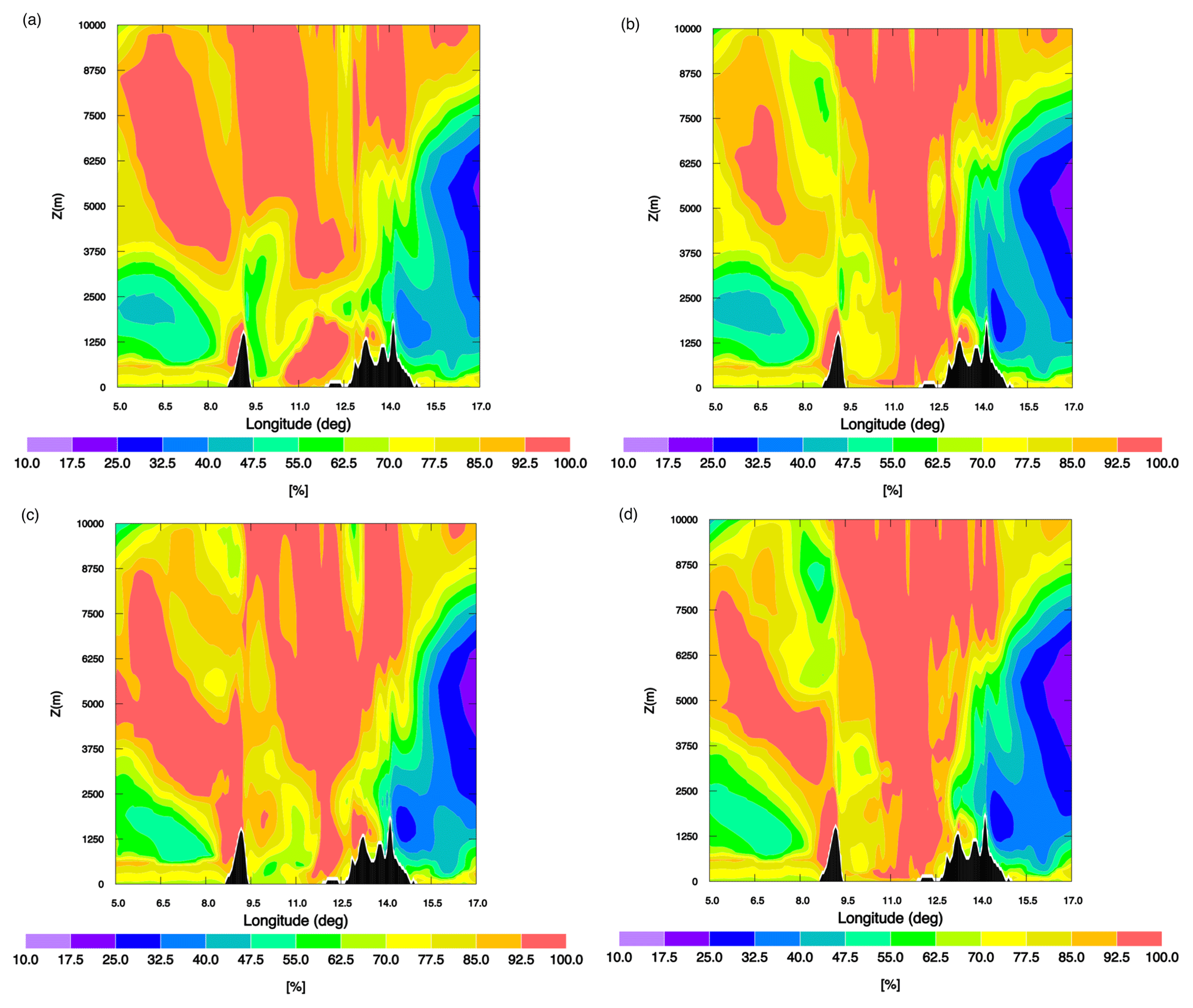
Figure 19Relative humidity longitude–height cross section at 42∘ N and at 06:00 UTC on 10 September 2017 for (a) CTRL, (b) RAD, (c) LIGHT, and (d) RADLI. Only the longitude range between 5 and 17∘ E and the vertical range between 0 and 10 km are shown for clarity.
Comparing RAD and CTRL the difference of the relative humidity field over the Tyrrhenian Sea and western part of Italy is evident (more specifically at longitudes between 10.5 and 12.5).
LIGHT shows two areas with high relative humidity: west of Corsica and over the Tyrrhenian Sea. The wet area west of Corsica is caused by the assimilation of lightning (Fig. 8b) and it is not simulated by RAD because Corsica is not well sampled by the radar network and because of different model evolutions. Lightning data assimilation also increases the humidity over the Tyrrhenian Sea and over the western part of Italy, as shown by the comparison with CTRL; nevertheless its effect is lower compared to radar reflectivity factor data assimilation.
RADLI has features of both lightning and radar reflectivity factor data assimilation.
So, considering the results of Figs. 18 and 19 as well as the rainfall VSF, the impact of lightning and radar reflectivity factors on the VSF can be very different despite both adjusting the water vapour mixing ratio.
In this paper, we showed the impact of lightning and radar reflectivity factor data assimilation on the very short-term precipitation forecast (3 h) for two case studies that occurred in Italy. We used the RAMS@ISAC model, whose 3D-Var extension to the assimilation of radar reflectivity factor is shown in this paper for the first time.
The first case study occurred on 16 September 2017 and it is a moderate case with localized rainfall over central Italy. It was chosen because the control forecast, i.e. without radar reflectivity factor or lightning data assimilation, missed the event. The second event, occurring on 9–10 September 2017, was characterized by exceptional rainfall over several parts of Italy. This event was partially represented by the control forecast. In particular, the forecast of the event was incorrect because (a) the control forecast was delayed compared to the observations and (b) the control forecast missed the rainfall over central Italy (Lazio Region).
It is important to recall that the impact of the lightning data assimilation on the precipitation forecast of RAMS@ISAC was already studied for the HyMeX-SOP1 period (Federico et al., 2017a, b), and a robust statistic is already available. The results of this study confirm the important role of the lightning data assimilation on the rainfall forecast for the other two case studies. However, considering the assimilation of radar reflectivity factor, and its combination with lightning data assimilation in RAMS@ISAC, the results of this paper are new.
Because we analysed only two case studies, no definitive conclusions can be derived on the performance of RAMS@ISAC with radar reflectivity factor data assimilation. There are, however, a few points worth mentioning.
The VSF performance of RAMS@ISAC is systematically improved by the assimilation of radar reflectivity factor. This improvement is of paramount importance for some specific VSFs (for example for the 00:00–03:00 UTC of Livorno), when the control forecast missed the event while it was correctly predicted by radar reflectivity factor data assimilation. Sometimes the improvement of reflectivity factor data assimilation has a small impact on the precipitation forecast, as for the period 18:00–21:00 UTC on 9 September 2017 (Livorno, not shown; see the discussion paper Federico et al. (2018) for a description of this VSF). This suggests that there is room for improvement for all components of the VSF: observations, data assimilation, and meteorological model.
Lightning and radar observations are different and both add value to the VSF. Some examples have been shown: the light precipitation over northern Italy for Serrano forecasted assimilating radar reflectivity factor well, while it does not simulate assimilating flashes because they are too few in this area to force convection; lightning data assimilation represents the deep convection occurring during the intense phase of the Livorno case better (00:00–03:00 UTC), especially because it is able to force convection where it occurs, reducing false alarms. The ability of lightning data assimilation to reduce false alarms compared to RAD and RADLI is shown by the fact that the ETS score for LIGHT is sometimes the best among all simulations (see also Sect. S2). These results also show that the influence of different observations depends on the meteorological situation.
The model configuration assimilating both radar reflectivity factor and lightning (RADLI) is able to retain important features of both data assimilations. For example, the simulation of the Livorno case in the phase 06:00–09:00 UTC was able to simulate the heavy precipitation over Lazio thanks to the radar reflectivity factor data assimilation and the precipitation over Sardinia, as well as the moderate precipitation over the central Alps, thanks to lightning data assimilation.
The property of RADLI to retain the precipitation features of both RAD and LIGHT is shown by the POD score, which is the best, for most cases and thresholds, for RADLI.
Another interesting feature is the considerable improvement of the POD of RADLI compared to CTRL for the lowest thresholds.
It is also underlined that the data assimilated, both lightning and radar reflectivity factor, are available in real time and could be used for an operational implementation of the VSF.
It is worth noting that several sensitivity tests were conducted for the case studies, whose results are shown in the Supplement. In particular, we studied the sensitivity of the rainfall VSF to (a) nudging formulation used for lightning data assimilation, (b) increasing the observation error of radar reflectivity factor, (c) changing the shape of the searching area to compute the relative humidity pseudo-profiles, (d) updating initial and boundary conditions (IC and BC) as new observations are available, and (e) increasing the vertical resolution of RAMS@ISAC by using 42 vertical levels. All these sensitivity tests confirm the findings of this paper.
The above results are promising and deserve future studies to better understand the role of radar reflectivity factor data assimilation and its interaction with lightning data assimilation to improve the precipitation forecast, especially at the very short range (0–3 h).
There are, however, less satisfactory aspects of assimilating both radar reflectivity factor and lightning data. In particular, the wet bias of RAD and RADLI forecast is the main drawback of the results of this paper. To reduce the moisture added by radar and lightning data assimilation, further research is needed and different approaches are possible (Fierro et al., 2016). In particular, (a) assimilating for a shorter time (0–6 h in this paper), (b) reducing the length scales of the 3D-Var in the horizontal directions to limit the spreading of the innovations, or assuming an innovation equal to zero for grid points without lightning and with zero reflectivity factor, (c) reducing the amount of water vapour added to the model (for example reducing the values of A and B constants for lightning data assimilation or relaxing the request of saturation when radar reflectivity is observed in areas where the model has zero reflectivity), and (d) adding moisture to a shallower vertical layer are options.
It is also noted that a combination of heating and moistening could provide the same buoyancy with less water vapour addition (Marchand and Fuelberg, 2014) and this approach could be used in future studies.
In addition to the acquisition of more case studies, there are two directions of future development of this work. The lightning data assimilation can be formulated by 3D-Var, using a strategy similar to the radar reflectivity factor in which pseudo-profiles of relative humidity are first generated where flashes are recorded and then assimilated by 3D-Var. This methodology was already reported in Fierro et al. (2016). The assimilation of both radar reflectivity factor and lightning using RAMS-3DVar will be explored in future studies.
Another important point to study is how long the innovations introduced by data assimilation last in the forecast. While in this study we consider the VSF at 3 h, future studies must explore longer time ranges. This kind of study was performed for lightning data assimilation (Fierro et al., 2015; Federico et al., 2017b; Lynn et al., 2015, among others) and for radar data assimilation (Hu et al., 2006; Jones et al., 2014, among others), using a rationale similar to that used in this paper.
In general, the performance of the forecast and the impact of lightning and radar data assimilation decrease with forecast range because boundary conditions propagate inside the domain and because model errors grow and eventually become dominant. Improving the data assimilation system also contributes to a longer resilience of model performance. The studies cited above showed that lightning and radar data assimilation can have an impact up to 24 h depending on several factors (meteorological model, data assimilation, quality of the data, meteorological conditions, initial and boundary conditions).
A study considering both radar reflectivity factor and lightning should be performed to understand the resilience of the innovations introduced by data assimilation.
The output of the RAMS@ISAC model and RAMS-3DVar are available upon request to the corresponding author. Radar and rain gauge data can be requested from the Department of Civil Protection (see the authors addresses). LINET data can be requested from Nowcast (https://www.nowcast.de, nowcast, 2019).
The supplement related to this article is available online at: https://doi.org/10.5194/nhess-19-1839-2019-supplement.
The idea of the study followed from discussions between SF and SD. The model and the RAMS-3DVar simulations were performed by SF, RCT, and EA. The data assimilation of radar reflectivity factor and radar data analysis were carried out by LB, OC, MM, and GV. Lightning data assimilation was performed by SF and SD. All authors contributed to writing and reviewing the paper.
The authors declare that they have no conflict of interest.
This article is part of the special issue “Hydrological cycle in the Mediterranean (ACP/AMT/GMD/HESS/NHESS/OS inter-journal SI)”. It is not associated with a conference.
This work is a contribution to the HyMeX programme. Part of the computational time used for this paper was granted by the ECMWF (European Centre for Medium-Range Weather Forecasts) throughout the special project SPITFEDE. LINET data were provided by Nowcast GmbH (https://www.nowcast.de/) within a scientific agreement between Hans Dieter Betz and the Satellite Meteorological Group of CNR-ISAC in Rome.
We acknowledge the three anonymous reviewers and the editor for the substantial improvement of the quality of the paper in the review process.
This work was partially funded by the agreement between CNR-ISAC and the Italian Department of Civil Protection.
This paper was edited by Christian Barthlott and reviewed by three anonymous referees.
Alexander, G. D., Weinman, J. A., Karyampoudi, V. M., Olson, W. S., and Lee, A. C. L.: The effect of assimilating rain rates derived from satellites and lightning on forecasts of the 1993 superstorm, Mon. Weather Rev., 127, 1433–1457, 1999.
Barker, D. M., Huang, W., Guo, Y.-R., and Xiao, Q. N.: A Three-Dimensional Variational Data Assimilation System for MM5: Implementation And Initial Results, Mon. Weather Rev., 132, 897–914, 2004.
Barker, D. M., Huang, X.-Y., Liu, Z., Aulignè, T., Zhang, X., Rugg ,S., Ajjaji, R., Bourgeois, A., Bray, J., Chen ,Y., Demirtas, M.,. Guo, Y.-R, Henderson, T., Huang, W, Lin, H. C., Michalakes, J., Rizvi, S., and Zhang, X.: The Weather Research and Forecasting (WRF) Model's Community Variational/Ensemble Data Assimilation System: WRFDA, B. Am. Meteorol. Soc., 93, 831–843, 2012.
Betz, H.-D., Schmidt, K., Oettinger, P., and Wirz, M.: Lightning detection with 3D-discrimination of intracloudandcloud-to-grounddischarges, J. Geophys. Res. Lett., 31, L11108, https://doi.org/10.1029/2004GL019821, 2004.
Betz, H. D., Schmidt, K., Laroche, P., Blanchet, P., Oettinger, P., Defer, E., Dziewit, Z., and Konarski, J.: LINET-an international lightning detection network in Europe, Atmos. Res., 91, 564–573, 2009.
Buzzi, A. and Tibaldi, S.: Cyclogenesis in the lee of the Alps: A case study, Q. J. Roy. Meteor. Soc., 104, 271–287, https://doi.org/10.1002/qj.49710444004, 1978.
Carey, L. D. and Rutledge, S. A.: Electrical and multiparameter radar observations of a severe hailstorm, J. Geophys. Res., 103, 13979–14000, https://doi.org/10.1029/97JD02626, 1998.
Caumont, O., Ducrocq, V., Wattrelot, E., Jaubert, G., and Pradier-Vabre, S.: 1D+3DVar assimilation of radar reflectivity data: a proof of concept, Tellus A, 62, 173–187, https://doi.org/10.1111/j.1600-0870.2009.00430.x, 2010.
Chang, D. E., Weinman, J. A., Morales, C. A., and Olson, W. S.: The effect of spaceborn microwave and ground-based continuous lightning measurements on forecasts of the 1998 Groundhog Day storm, Mon. Weather Rev., 129, 1809–1833, 2001.
Chen, C. and Cotton, W. R.: A One-Dimensional Simulation of the Stratocumulus-Capped Mixed Layer, Bound.-Lay. Meteorol., 25, 289–321, 1983.
Cotton, W. R., Pielke Sr., R. A., Walko, R. L., Liston, G. E., Tremback, C. J., Jiang, H., McAnelly, R. L., Harrington, J. Y., Nicholls, M. E., Carrio, G. G., and McFadden, J. P.: RAMS 2001: Current status and future directions, Meteorol. Atmos. Phys., 82, 5–29, 2003.
Courtier, P., Thépaut, J. N., and Hollingsworth, A.: A strategy for operational implementation of 4D-Var, using an incremental approach, Q. J. Roy. Meteor. Soc., 120, 1367–1387, 1994.
Dahl, J. M. L., Höller, H., and Schumann, U.: Modeling the Flash Rate of Thunderstorms. Part II: Implementation, Mon. Weather Rev., 139, 3112–3124, 2011.
Deierling, W. and Peterse, W. A.: Total lightning activity as an indicator of updraft characteristics, J. Geophys. Res., 113, D16210, https://doi.org/10.1029/2007JD009598, 2008.
Ducrocq, V., Braud, I., Davolio, S., Ferretti, R., Flamant, C., Jansa, A., Kalthoff, N., Richard, E., Taupier-Letage, I., Ayral, P.-A., Belamari, S., Berne, A., Borga, M., Boudevillain, B., Bock, O., Boichard, J.-L., Bouin, M.-N., Bousquet, O., Bouvier, C., Chiggiato, J., Cimini, D., Corsmeier, U., Coppola, L., Cocquerez, P., Defer, E., Delanoë, J., Di Girolamo, P., Doerenbecher, A., Drobinski, P., Dufournet, Y., Fourrié, N., Gourley, J.J., Labatut, L., Lambert, D., Le Coz, J., Marzano, F.S., Molinié, G., Montani, A., Nord, G., Nuret, M., Ramage, K., Rison, W., Roussot, O., Said, F., Schwarzenboeck, A., Testor, P., Van Baelen, J., Vincendon, B., Aran, M., and Tamayo, J.: HYMEX-SOP1 The Field Campaign Dedicated to Heavy Precipitation and Flash Flooding in the Northwestern Mediterranean, B. Am. Meteorol. Soc., 95, 1083–1100, https://doi.org/10.1175/BAMS-D-12-00244.1, 2014.
Emersic, C., and Saunders, C. P. R.: Further laboratory investigations into the relative diffusional growth rate theory of thunderstorm electrification, Atmos. Res., 98, 327–340, https://doi.org/10.1016/j.atmosres.2010.07.011, 2010.
Fabry, F. and Sun, J.: For how long should what data be assimilated for the mesoscale forecasting of convection and why? Part I: On the propagation of initial condition errors and their implications for data assimilation, Mon. Weather Rev., 138, 242–255, 2010.
Federico, S.: Implementation of a 3D-Var system for atmospheric profiling data assimilation into the RAMS model: initial results, Atmos. Meas. Tech., 6, 3563–3576, https://doi.org/10.5194/amt-6-3563-2013, 2013.
Federico, S.: Implementation of the WSM5 and WSM6 Single Moment Microphysics Scheme into the RAMS Model: Verification for the HyMeX-SOP1, Adv. Meteorol., 2016, 17 pp., https://doi.org/10.1155/2016/5094126, 2016.
Federico, S., Avolio, E., Petracca, M., Panegrossi, G., Sanò, P., Casella, D., and Dietrich, S.: Simulating lightning into the RAMS model: implementation and preliminary results, Nat. Hazards Earth Syst. Sci., 14, 2933–2950, https://doi.org/10.5194/nhess-14-2933-2014, 2014.
Federico, S., Petracca, M., Panegrossi, G., and Dietrich, S.: Improvement of RAMS precipitation forecast at the short-range through lightning data assimilation, Nat. Hazards Earth Syst. Sci., 17, 61–76, https://doi.org/10.5194/nhess-17-61-2017, 2017a.
Federico, S., Petracca, M., Panegrossi, G., Transerici, C., and Dietrich, S.: Impact of the assimilation of lightning data on the precipitation forecast at different forecast ranges, Adv. Sci. Res., 14, 187–194, 2017b.
Federico, S., Torcasio, R. C., Avolio, E., Caumont, O., Montopoli, M., Baldini, L., Vulpiani, G., and Dietrich, S.: The impact of lightning and radar data assimilation on the performance of very short term rainfall forecast for two case studies in Italy, Nat. Hazards Earth Syst. Sci. Discuss., https://doi.org/10.5194/nhess-2018-319, in review, 2018.
Ferretti, R., Pichelli, E., Gentile, S., Maiello, I., Cimini, D., Davolio, S., Miglietta, M. M., Panegrossi, G., Baldini, L., Pasi, F., Marzano, F. S., Zinzi, A., Mariani, S., Casaioli, M., Bartolini, G., Loglisci, N., Montani, A., Marsigli, C., Manzato, A., Pucillo, A., Ferrario, M. E., Colaiuda, V., and Rotunno, R.: Overview of the first HyMeX Special Observation Period over Italy: observations and model results, Hydrol. Earth Syst. Sci., 18, 1953–1977, https://doi.org/10.5194/hess-18-1953-2014, 2014.
Fierro, A. O., Gilmore, M. S., Mansell, E. R., Wicker, L. J., and Straka, J. M.: Electrification and lightning in an idealized boundary-crossing supercell simulation of 2 June 1995, Mon. Weather Rev., 134, 3149–3172, https://doi.org/10.1175/MWR3231.1, 2006.
Fierro, A. O., Mansell, E., Ziegler, C., and MacGorman, D.: Application of a lightning data assimilation technique in the WRFARW model at cloud-resolving scales for the tornado outbreak of 24 May 2011, Mon. Weather Rev., 140, 2609–2627, 2012.
Fierro, A. O., Gao, J., Ziegler, C., Mansell, E. R., MacGorman, D. R., and Dembek, S.: Evaluation of a cloud scale lightning data assimilation technique and a 3DVAR method for the analysis and short-term forecast of the 29 June 2012 derecho event, Mon. Weather Rev., 142, 183–202, https://doi.org/10.1175/MWR-D-13-00142.1, 2014.
Fierro, A. O., A. J. Clark, E. R. Mansell, D. R. MacGorman, S. Dembek, and C. Ziegler: Impact of storm-scale lightning data assimilation on WRF-ARW precipitation forecasts during the 2013 warm season over the contiguous United States, Mon. Weather Rev., 143, 757–777, https://doi.org/10.1175/MWR-D-14-00183.1, 2015.
Fierro, A. O., Gao, L., Ziegler, C. L., Calhoun, K. M., Mansell, E. R., and MacGorman, D. R.: Assimilation of Flash Extent Data in the Variational Framework at Convection-Allowing Scales: Proof-of-Concept and Evaluation for the Short-Term Forecast of the 24 May 2011 Tornado Outbreak, Mon. Weather Rev., 144, 4373–4393, https://doi.org/10.1175/MWR-D-16-0053.1, 2016.
Giannaros, T. M., Kotroni, V., and Lagouvardos, K.: WRFLTNGDA: A lightning data assimilation technique implemented in the WRF model for improving precipitation forecasts, Environ. Model. Softw., 76, 54–68, https://doi.org/10.1016/j.envsoft.2015.11.017, 2016.
Hong, S. Y. and Lim, J. J. O.: The WRF single-moment 6-class microphysics scheme (WSM6), J. Korean Meteorol. Soc., 42, 129–151, 2006.
Hu, M., Xue, M., and Brewster, K.: 3DVAR and cloud analysis with WSR-88D level-II data for the prediction of the Fort Worth, Texas, tornadic thunderstorms. Part I: Cloud analysis and its impact, Mon. Weather Rev., 134, 675–698, https://doi.org/10.1175/MWR3092.1, 2006.
Ikuta, Y. and Honda, Y.: Development of 1D+4DVAR data assimilation of radar reflectivity in JNoVA. Tech, Report, 01.09–01.10, available at: http://www.wcrp-climate.org/WGNE/BlueBook/2011/individual-articles/01_Ikuta_Yasutaka_WGNE2011_1D4DVAR.pdf (last access: 8 August 2019), 2011.
Jones, C. D. and Macpherson, B.: A latent heat nudging scheme for the assimilation of precipitation into an operational mesoscale model, Meteorol. Appl., 4, 269–277, 1997.
Jones, T. A., Otkin, J. A., Stensrud, D. J., and Knopfmeier, K.: Forecast evaluation of an observing system simulation experiment assimilating both radar and satellite data, Mon. Weather Rev., 142, 107–124, https://doi.org/10.1175/MWR-D-13-00151.1, 2014.
Kain, J. S. and Fritsch, J. M.: Convective parameterization for mesoscale models: the Kain-Fritsch scheme. The representation of cumulus convection in numerical models, Meteor. Monogr. No. 46, Am. Meteor. Soc., Boston, 165–170, 1993.
Kuhlman, K. M., Zielger, C. L., Mansell, E. R., MacGorman, D. R., and Straka, J. M.: Numerically simulated electrification and lightning of the 29 June 2000 STEPS supercell storm, Mon. Weather Rev., 134, 2734–2757, https://doi.org/10.1175/MWR3217.1, 2006.
Kummerow, C., Hong, Y., Olson, W. S., Yang. S., Adler, R. F., McCollum, J., Ferraro, R., Petty, G., Shin. D.-B., and Wilheit, T. T.: The evolution of the Goddard profiling algorithm (GPROF) for rainfall estimation from passive microwave sensors, J. Appl. Meteorol., 40, 1801–1820, 2001.
Lagouvardos, K., Kotroni, V., Betz, H.-D., and Schmidt, K.: A comparison of lightning data provided by ZEUS and LINET networks over Western Europe, Nat. Hazards Earth Syst. Sci., 9, 1713–1717, https://doi.org/10.5194/nhess-9-1713-2009, 2009.
Lynn, B. H.: The Usefulness and Economic Value of Total Lightning Forecasts Made with a Dynamic Lightning Scheme Coupled with Lightning Data Assimilation, Weather Forecast., 32, 645–663, https://doi.org/10.1175/WAF-D-16-0031.1, 2017.
Lynn, B. H., Kelman, G., and Ellrod, G.: An evaluation of the ef?cacy of using observed lightning to improve convective lightning forecasts, Weather Forecast., 30, 405–423 https://doi.org/10.1175/WAF-D-13-00028.1, 2015.
MacGorman, D. R. and Nielsen, K. E.: Cloud-to-Ground Lightning in a Tornadic Storm on 8 May 1986, Mon. Weather Rev., 119, 1557–1574, https://doi.org/10.1175/1520-0493(1991)119<1557:CTGLIA>2.0.CO;2, 1991.
MacGorman, D. R., Burgess, D. W., Mazur, V., Rust, W. D., Taylor, W. L., and Johnson, B. C.: Lightning rates relative to tornadic storm evolution on 22 May 1981, J. Atmos. Sci., 46, 221–251, https://doi.org/10.1175/1520-0469(1989)046<0221:LRRTTS>2.0.CO;2, 1989.
MacGorman, D. R., Apostolakopoulos, I. R., Lund, N. R., Demetriades, N. W. S., Murphy, M. J., and Krehbiel, P. R.: The timing of cloud-to-ground lightning relative to total lightning activity, Mon. Weather Rev., 139, 3871–3886, https://doi.org/10.1175/MWR-D-11-00047.1, 2011.
MacGorman, D. R., Apostolakopoulos, I. R., Lund, N. R., Demetriades, N. W. S., Murphy, M. J., and Krehbiel, P. R.: The electrical structure of two supercell storms during STEPS, Mon. Weather Rev., 133, 2583–2607, https://doi.org/10.1175/MWR2994.1, 2005.
Mansell, E. R., Ziegler, C. L., and MacGorman, D. R.: A lightning data assimilation technique for mesoscale forecast models, Mon. Weather Rev., 135, 1732–1748, 2007.
Marchand, M. and Fuelberg, H.: Assimilation of lightning data using a nudging method involving low-level warming, Mon. Weather Rev., 142, 4850–4871, https://doi.org/10.1175/MWR-D-14-00076.1, 2014.
Mass, C. F., Ovens, D., Westrick, K., and Colle, B. A.: Does increasing horizontal resolution produce more skilful forecasts?, B. Am. Meteorol. Soc., 83, 407–430, 2002.
Mellor, G. and Yamada, T.: Development of a Turbulence Closure Model for Geophysical Fluid Problems, Review of Geophysics and Space Physics, 20, 851–875, 1982.
Mittermaier, M., Roberts, N., and Thompson, S. A.: A long-term assessment of precipitation forecast skill using the Fractions Skill Score, Meteor. Appl., 20, 176–186, https://doi.org/10.1002/met.296, 2013.
Molinari, J. and Corsetti, T.: Incorporation of cloud-scale and mesoscale down-drafts into a cumulus parametrization: results of one and three-dimensional integrations, Mon. Weather Rev., 113, 485–501, 1985.
nowcast: available at: https://www.nowcast.de, last access: 8 August 2019.
Olson, W. S., Kummerow, C. D., Heymsfield, G. M., and Giglio, L.: A method for combined passive-active microwave retrievals of cloud and precipitation profiles, J. Appl. Meteorol., 35, 1763–1789, 1996.
Papadopoulos, A., Chronis, T. G., and Anagnostou, E. N.: Improving convective precipitation forecasting through assimilation of regional lightning measurements in a mesoscale model, Mon. Weather Rev., 133, 1961–1977, 2005.
Parrish, D. F. and Derber, J. C.: The National Meteorological Center's Spectral Statistical Interpolation analysis system, Mon. Weather Rev., 120, 1747–1763, 1992.
Pessi, A. T. and Businger, S.: Relationships among Lightning, Precipitation, and Hydrometeor Characteristics over the North Pacific Ocean, J. Appl. Meteor. Clim., 48, 833–848, https://doi.org/10.1175/2008JAMC1817.1, 2009.
Petracca, M., Casella, D., Dietrich, S., Milani, L., Panegrossi, G., Sanò, P., Möhrlein, M., Riso, S., and Betz, H. D.: Lightning strokes frequency homogenization for climatological analysis: application to LINET data records over Europe, 2nd TEA – IS Summer School, 23–27 June, Collioure, France, 2014.
Petracca, M., D'Adderio, L. P., Porcù, F., Vulpiani, G., Sebastianelli, S., and Puca, S.: Validation of GPM Dual-Frequency Precipitation Radar (DPR) rainfall products over Italy, J. Hydrometeorol., 19, 907–925, https://doi.org/10.1175/JHM-D-17-0144.1, 2018.
Press, W. H., Teukolsky, S. A., Vetterling, W. T., and Flannery, B. P.: Numerical recipes in Fortran 77, second ed., Cambridge University Press, Cambridge, 992 pp., 1992.
Qie, X., Zhu, R., Yuan, T., Wu, X., Li, W., and Liu, D.: Application of total-lightning data assimilation in a mesoscale convective system based on the WRF model, Atmos. Res., 145–146, 255–266, 2014.
Ricciardelli, E., Di Paola, F., Gentile, S., Cersosimo, A., Cimini, D., Gallucci, D., Geraldi, E., Larosa, S., Nilo, S. T., Ripepi, E., Romano, F., and Viggiano, M.: Analysis of Livorno Heavy Rainfall Event: Examples of Satellite-Based Observation Techniques in Support of Numerical Weather Prediction, Remote Sensing, 2018, 1549, https://doi.org/10.3390/rs10101549, 2018.
Ridal, M. and Dahlbom, M.: Assimilation of multinational radar reflectivity data in a mesoscale model: a proof of concept, J. Appl. Meteorol. Clim., 56, 1739–1751, https://doi.org/10.1175/jamc-d-16-0247.1, 2017.
Roebber, P. J.: Visualizing multiple measures of forecast quality, Weather Forecast., 24, 601–608, 2009.
Rohn, M., Kelly, G., and Saunders, R. W.: Impact of a New Cloud Motion Wind Product from Meteosat on NWP Analyses and Forecasts, Mon. Weather Rev., 129, 2392–2403, 2001.
Smagorinsky, J.: General circulation experiments with the primitive equations. Part I, The basic experiment, Mon. Weather Rev., 91, 99–164, 1963.
Stensrud, D. J. and Fritsch, J. M.: Mesoscale convective systems in weakly forced large-scale environments. Part II: Generation of a mesoscale initial condition, Mon. Weather Rev., 122, 2068–2083, 1994.
Stensrud, D. J., Xue, M., Wicker, L. J., Kelleher, K. E., Foster, M. P., Schaefer, J. T., Schneider, R. S., Benjamin, S. G., Weygandt, S. S., Ferree, J. T., and Tuell, J. P.: Convective-Scale Warn-on-Forecast System, B. Am. Meteorol. Soc., 90, 1487–1500, https://doi.org/10.1175/2009BAMS2795.1, 2009.
Stewart, L. M., Dance, S. L., and Nichols, N. K.: Data assimilation with correlated observation errors: experiments with a 1-D shallow water model, Tellus A, 65, 19546, https://doi.org/10.3402/tellusa.v65i0.19546, 2013.
Sun, J. and Crook, N. A.: Dynamical and Microphysical Retrieval from Doppler RADAR Observations Using a Cloud Model and Its Adjoint, Part I: Model Development and Simulated Data Experiments, J. Atmos. Sci., 54, 1642–1661, 1997.
Sun, J. and Crook, N. A.: Dynamical and Microphysical Retrieval from Doppler RADAR Observations Using a Cloud Model and Its Adjoint, Part II: Retrieval Experiments of an Observed Florida Convective Storm, J. Atmos. Sci., 55, 835–852, 1998.
Takahashi, T.: Riming electrification as a charge generation mechanism in thunderstorms, J. Atmos. Sci., 35, 1536–1548, https://doi.org/10.1175/1520-0469(1978)035<1536:REAACG>2.0.CO;2, 1978.
Vulpiani, G., Rinollo, A., Puca, S., and Montopoli, M.: A quality-based approach for radar rain field reconstruction and the H-SAF precipitation products validation. Proc. Eighth European Radar Conf., Garmish-Partenkirchen, Germany, ERAD, Abstract 220, 6 pp., available at: http://www.pa.op.dlr.de/erad2014/programme/ExtendedAbstracts/220_Vulpiani.pdf (last access: 8 August 2019), 2014.
Walko, R. L., Band, L. E., Baron, J., Kittel, T. G., Lammers, R., Lee, T. J., Ojima, D., Pielke Sr., R. A., Taylor, C., Tague, C., Tremback, C. J., and Vidale, P. L.: Coupled Atmosphere-Biosphere-Hydrology Models for environmental prediction, J. Appl. Meteorol., 39, 931–944, 2000.
Wattrelot, É., Caumont, O., and Mahfouf, J. F.: Operational implementation of the 1D+3D-Var assimilation method of radar reflectivity data in the AROME model, Mon. Weather Rev., 142, 1852–1873, https://doi.org/10.1175/MWR-D-13-00230.1, 2014.
Weisman, M. L., Skamarock, W. C., and Klemp, J. B.: The resolution dependence of explicitly modeled convective systems, Mon. Weather Rev., 125, 527–548, 1997.
Weygandt, S. S., Benjamin, S. G., Hu, M., Smirnova, T. G., and Brown, J. M.: Use of lightning data to enhance radar assimilation within the RUC and Rapid Refresh models. Third Conf. on Meteorological Applications of Lightning Data, 20–24 January 2008, New Orleans, LA, Amer. Meteor. Soc., 8.4, available at: https://ams.confex.com/ams/88Annual/webprogram/Paper134112.html (last access: 3 October 2018), 2008.
Wiens, K. C., Rutledge, S. A., and Tessendorf, S. A.: The 29 June 2000 supercell observed during STEPS. Part II: Lightning and charge structure, J. Atmos. Sci., 62, 4151–4177, https://doi.org/10.1175/JAS3615.1, 2005.
Wilks, D. S.: Statistical Methods in the Atmospheric Sciences, Academic Press, London, 627 pp., 2006.
Xu, Q., Wei, L., Gu, W., Gong, J., and Zhao, Q.: A 3.5-dimensional variational method for Doppler radar data assimilation and its application to phased array radar observations, Adv. Meteorol., 2010, 797265, https://doi.org/10.1155/2010/797265, 2010.
Xue, M., Wang, D., Gao, J., Brewster, K., and Droegemeier, K. K.: The Advanced Regional Prediction System (ARPS), storm scale numerical weather prediction and data assimilation, Meteorol. Atmos. Phys., 82, 139–170, 2003.
Zhao, Q., Cook, J., Xu, Q., and Harasti, P. R.: Using radar wind observations to improve mesoscale numerical weather prediction, Weather Forecast., 21, 502–522, 2006.
Throughout the paper we use the expression radar reflectivity factor, which is the quantity provided by the radar (and expressed in millimetres to the sixth power per cubic metre or Z) after conversion from the received power. The radar reflectivity factor is different from reflectivity and is obtained in the special case of Rayleigh scattering. Reflectivity is not the quantity that radars usually provide and display on their screens, although most people refer to it.