California earthquake insurance unpopularity:  the issue is the price, not the risk perception

Pothon, Adrien; Gueguen, Philippe; Buisine, Sylvain; Bard, Pierre-Yves

doi:https://doi.org/10.5194/nhess-19-1909-2019

Articles | Volume 19, issue 8

https://doi.org/10.5194/nhess-19-1909-2019

Articles | Volume 19, issue 8

Research article

29 Aug 2019

Research article |

| 29 Aug 2019

California earthquake insurance unpopularity: the issue is the price, not the risk perception

Adrien Pothon, Philippe Gueguen, Sylvain Buisine, and Pierre-Yves Bard

Abstract

Despite California being a highly seismic prone region, most homeowners are not covered against this risk. This study analyses the reasons for homeowners to purchase insurance to cover earthquake losses, with application in California. A dedicated database is built from 18 different data sources about earthquake insurance, gathering data since 1921. A new model is developed to assess the take-up rate based on the homeowners’ risk awareness and the average annual insurance premium amount. Results suggest that only two extreme situations would lead all owners to cover their home with insurance: (1) a widespread belief that a devastating earthquake is imminent, or alternatively (2) a massive decrease in the average annual premium amount by a factor exceeding 6 (from USD 980 to 160, 2015 US dollars). Considering the low likelihood of each situation, we conclude from this study that new insurance solutions are necessary to fill the protection gap.

Download & links

Article (PDF, 1423 KB)

Supplement (60 KB)

Download & links

Article (1423 KB)
Supplement (60 KB)
BibTeX
EndNote

How to cite

How to cite.

Dates

Received: 01 Feb 2019 – Discussion started: 08 Feb 2019 – Revised: 01 Aug 2019 – Accepted: 02 Aug 2019 – Published: 29 Aug 2019

1 Introduction

Since 2002, the rate of homeowners insured against earthquake risk in California has never exceeded 16 %, according to data provided by the California Department of Insurance (CDI, 2017b, California Insurance Market Share Reports). Such a low rate is surprising in a rich area prone to earthquake risk. Consequently, several studies have already investigated homeowners' behaviour regarding earthquake insurance in California, in order to identify people who might have an interest in purchasing earthquake insurance and to understand why they do not do so. Three main variables have been observed as decisive in purchasing an earthquake insurance: the premium amount, the socio-economic background and the risk perception (Kunreuther et al., 1978; Palm and Hodgson, 1992a; Wachtendorf and Sheng, 2002). For the premium amount, both a survey conducted by Meltsner (1978) and the statistics collected from insurance data by Buffinton (1961) and Latourrette et al. (2010) show, as expected, a negative correlation between the premium amount and the insurance adoption. Nevertheless, even uninsured homeowners tend to overestimate the loss they would face in case of a major event and feel vulnerable regardless of their income level (Kunreuther et al., 1978; Palm and Hodgson, 1992a). As they are not expecting much from federal aids, they do not know how they will recover (Kunreuther et al., 1978).

Consequently the decision to purchase insurance to cover earthquake losses is not correlated to the income level (Kunreuther et al., 1978; Wachtendorf and Sheng, 2002). Several other socio-economic factors (e.g. the duration of residence, the neighbours' behaviour, the communication strategies of mass media, real estate agencies and insurance companies) have an impact on the risk perception (Meltsner, 1978; Palm and Hodgson, 1992a; Lin, 2013).

Pricing methods used in the real estate market do not take into account seismic risk. Indeed, based on data from the World Housing Encyclopedia, Pothon et al. (2018) have shown that building construction price is not correlated to the seismic vulnerability rating. Moreover, earthquake insurance is not mandatory in California for residential mortgage (CDI, 2019, Information Guides, Earthquake Insurance). Still, lenders for commercial mortgages are used to requiring earthquake insurance only when the probable maximum loss is high (Porter et al., 2004). However, Porter et al. (2004) have shown that taking into account earthquake risk for calculating the building's net asset value can have a significant impact in earthquake-prone areas like California.

Also, people insured against earthquake risk can receive a compensation lower than the loss incurred because most earthquake insurance policies in California include a deductible amount (i.e. at the charge of the policyholder) and are calibrated based on a total reconstruction cost, declared by the policyholder. As reported by Marquis et al. (2017) after the 2010–2011 Canterbury (NZL) earthquakes, this amount can be inadequate for the actual repair costs. Both high deductible amount (Meltsner, 1978; Palm and Hodgson, 1992b; Burnett and Burnett, 2009) and underestimated total reconstruction cost (Garatt and Marshall, 2003) can make insured people feel unprotected after an earthquake, making this kind of insurance disrepute.

Since homeowners are aware of the destructive potential of a major earthquake, the risk perception reflects their personal estimate of the occurrence (Kunreuther et al., 1978; Wachtendorf and Sheng, 2002). Indeed, most of them disregard this risk because it is seldom, even if destructive earthquake experiences foster insurance underwriting during the following year (Buffinton, 1961; Kunreuther et al., 1978; Meltsner, 1978; Lin, 2015). Consequently, earthquake insurance purchasing behaviour is correlated with personal understanding of seismic risk and is not only related to scientific-based hazard level (Palm and Hodgson, 1992a; Palm, 1995; Wachtendorf and Sheng, 2002).

With limits in earthquake insurance consumption identified, the next step is to assess the contribution of each factor to the take-up rate. Kunreuther et al. (1978) first proposed a sequential model showing that the individual's purchasing behaviour depends on personal risk perception, premium amount and knowledge of insurance solutions. In the same study (Kunreuther et al., 1978), a numerical model was developed, at the same granularity, failing however to accurately reproduce the observed behaviours. According to the authors, the model failed because many surveyed people had a lack of knowledge of existing insurance solutions or were unable to quantify the risk. Models published later (Latourrette et al., 2010; Lin, 2013, 2015) assessed the take-up rate by postal code and used demographic variables to capture the disparity in insurance solution knowledge. Nevertheless because of lack of data, they assumed the premium amount or the risk perception as constant.

The main objective of this study is to introduce a new take-up rate model for homeowners at the scale of California state. Such spatial resolution allows work on most data available in financial reports, which are numerous enough to use both the premium amount and the risk perception as variables. Different from previous studies focusing on risk pricing (Yucemen, 2005; Petseti and Nektarios, 2012; Asprone et al., 2013), this study takes into account the homeowners' risk perception and behaviour. This shift in point of view approach changes the main issue from what the price of earthquake insurance should be considering the risk level to what the acceptable price for consumers to purchase an earthquake insurance cover is. Despite results being at the state level, they bring a new framework to model earthquake insurance consumption which allows us to quantify the gap between premium amount and homeowners' willingness to pay, depending on the homeowners' risk awareness. Last, this study is also innovative by separately modelling the contribution of the risk perception and the premium amount to the level of earthquake insurance consumption.

In the first section, data are collected from several sources, processed and summarized in a new database. A take-up rate model is then developed by introducing the two following explanatory variables: the average premium amount and the subjective annual occurrence probability, defined as the risk perceived by homeowners of being affected by a destructive earthquake in 1 year. The perceived annual probability of occurrence is then studied from 1926 to present, in the next section. Finally, the last section is dedicated to analysing the current low earthquake insurance take-up rate for California homeowners.

2 Data collection and processing

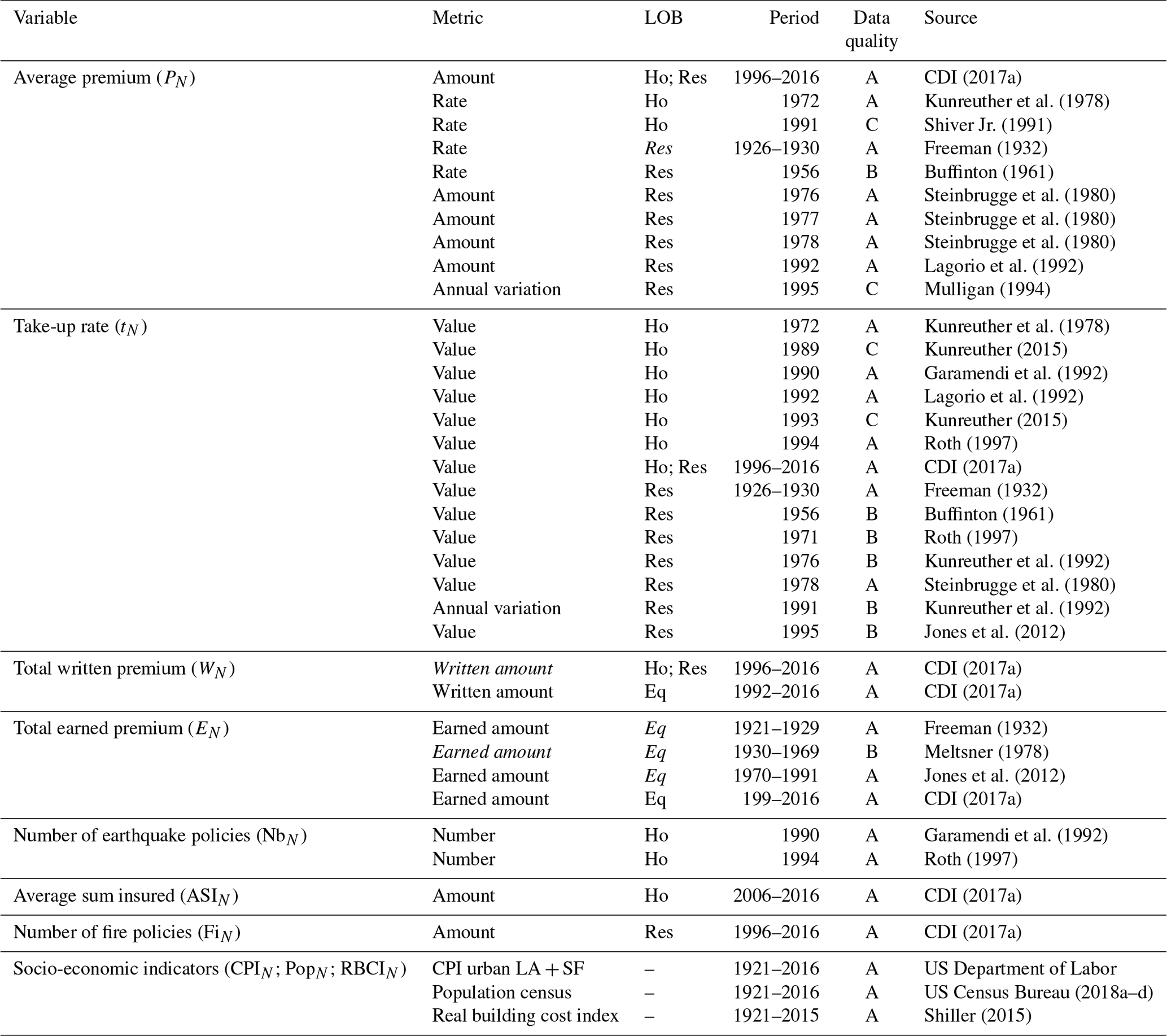
Developing such a model, even at the state level, faces a first challenge in data collection. Despite the California earthquake insurance market having been widely analysed, data volume before the 1990s remains low and extracted from scientific and mass media publications which refer to original data sources that are no longer available. As a consequence, data description is often sparse and incomplete and values can be subject to errors or bias. Consequently, data quality of each dataset has to be assessed. Here, it is done on the basis of the support (scientific publication or mass media), the data description (quality of information on the data type and the collecting process) and the number of records. The datasets with the highest quality are used and presented in Table 1 (values are available in the Supplement).

Table 1Raw data collected about earthquake insurance. Labels in italic are not extracted from publications but have been inferred by cross-checking with other sources. The data quality scale is A (good): scientific publication with methodology explained; B (acceptable): scientific publication without details on the methodology; C (weak): mass media. CPI: consumer price index; Eq: earthquake; Ho: homeowners; LA: Los Angeles; LOB: line of business; Res: residential; SF: San Francisco.

Download Print Version | Download XLSX

This study focuses on the following variables about earthquake insurance policies:

the total written premium (W_N), corresponding to the total amount paid by policyholders to insurance companies during the year N;
the take-up rate (t_N), defined as the ratio between the number of policies with an earthquake coverage (Nb_N) and those with a fire coverage (Fi_N);
the annual average premium (P_N), equal to W_N over Nb_N;
the average premium rate (p_N) equal to the ratio between the annual average premium amount P_N and the average value of the good insured (here a house), later referred to as the average sum insured (ASI_N).

All these variables can be calculated for any set of earthquake insurance policies. Insurance companies usually classify their products as follows: the residential line of business (Res) corresponds to insurance policies covering personal goods (e.g. house, condominium, mobile home, jewellery, furniture). The homeowners line of business corresponds to the insurance policies included in the residential line of business but dedicated to homeowners. As an earthquake insurance cover can be either a guarantee included in a wider policy (e.g. also covering fire or theft risks) or issued in a stand-alone policy, the earthquake line of business (Eq) classifies all insurance policies exclusively covering the earthquake risk. Some insurance policies within the earthquake line of business are dedicated to professional clients and do not belong to the residential line of business. For clarity, variables hold the title of the line of business when they are not related to the homeowners line of business.

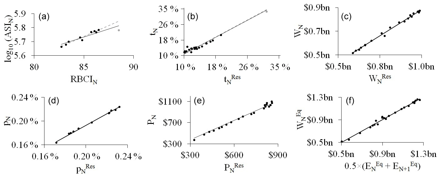
https://www.nat-hazards-earth-syst-sci.net/19/1909/2019/nhess-19-1909-2019-f01

Figure 1Fits of the linear regressions for (a) the average sum insured and the real building cost index, (b) the average premium rate between the residential and the homeowner lines of business, (c) the take-up rate between the residential and the homeowner lines of business, (d) the average premium amount between the residential and the homeowner lines of business, (e) the total written premium amount between the residential and the homeowner lines of business, and (f) the written and the earned premium amounts. Grey points on (a) and (c) represent the extreme values, affecting the linear regression from the solid black line to the dashed grey line, when removed. Financial values are in 2015 US dollars.

Download

Data for all the variables listed are available only since 1996 (Table 1). In order to expand the historical database, they are also estimated in an indirect way for the following periods: 1926–1930, 1956, 1971–1972, 1976–1978 and 1989–1995, leading us to consider additional data (Table 1) and to use linear regressions (Fig. 1).

By definition of the average premium rate (p_N), P_N can be approximated by the product of p_N and the average sum insured (ASI_N). The latter is estimated from the real building cost index (RBCI_N), which is an economic index (base: 31 December 1979=100) capturing the evolution of the cost of building construction works (Shiller, 2018). The following linear regression has been calibrated on data from Table 1 between 2006 and 2015:

\begin{matrix} (1) & \begin{aligned} \log_{10} ({ASI}_{N}) = & 0.0233 \times {RBCI}_{N} + 3.7554 \\ (R^{2} = 0.84 Fig . 1 a) \end{aligned}, \end{matrix}

where ASI_N is in 2015 US dollars and R² is the coefficient of determination. When the average premium rate corresponds to the residential line of business ( $p_{N}^{Res}$ ), it can be converted into p_N with the following linear regression built on the CDI database between 2006 and 2016 (Table 1):

\begin{matrix} (2) & p_{N} = 0.96 \times p_{N}^{Res} (R^{2} = 1 Fig . 1 b) . \end{matrix}

Again using the CDI database between 1996 and 2016 (Table 1), the following linear regressions have also been developed between P_N, t_N, and W_N and the corresponding metrics for the residential line of business ( $P_{N}^{Res}$ , $t_{N}^{Res}$ and $W_{N}^{Res})$ .

\begin{array}{l} (3) & t_{N} = 1.08 \times t_{N}^{Res} (R^{2} = 0.95 Fig . 1 c) \\ (4) & P_{N} = 1.24 \times P_{N}^{Res} (R^{2} = 0.99 Fig . 1 d) \end{array}

\begin{matrix} (5) & W_{N} = 0.88 \times W_{N}^{Res} (R^{2} = 0.99 Fig . 1 e) \end{matrix}

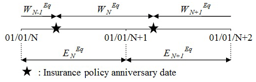
Before 1996, the total premium amount for earthquake insurance, mentioned in CDI (2017b) reports, was about the earthquake line of business, and in terms of total earned premium (E_N). While the total written premium (W_N) corresponds to the total amount of premium paid by policyholders to insurance companies during the year N, E_N is the amount of premium used to cover the risk during the year N. To illustrate these two definitions, Fig. 2 takes the example of an insurance policy for which the annual premium is paid 1 March every year. As the amount received at year N by the insurance company (W_N) covers the risk until 1 March, N+1, the insurance company can use only 75 % of W_N during the year N (9 months over 12). By adding the 25 % of W_N−1, this makes the total earned premium E_N, for the year N.

https://www.nat-hazards-earth-syst-sci.net/19/1909/2019/nhess-19-1909-2019-f02

Figure 2Illustration of the difference between the earned and the written premium amount.

Download

To estimate $W_{N}^{Eq}$ from $E_{N}^{Eq}$ for the earthquake line of business, the following relationship has been defined based on data from the CDI (2017a, b) database and over the period 1992–2016 (Table 1):

\begin{matrix} (6) & W_{N}^{Eq} = \frac{E_{N}^{Eq} + E_{N + 1}^{Eq}}{2} (R^{2} = 0.99 Fig . 1 f) . \end{matrix}

About the difference between $W_{N}^{Eq}$ and $W_{N}^{Res}$ , despite data (Table 1) showing a significant difference ( $W_{N}^{Eq} - W_{N}^{Res}$ = USD 250 m) since 1996, this study assumes that $W_{N}^{Eq}$ is equal to $W_{N}^{Res}$ until 1995, i.e.

\begin{matrix} (7) & W_{N}^{Res} = \approx \{\begin{cases} W_{N}^{Eq} & if N \leq 1995 \\ W_{N}^{Eq} - US 249 188 671 & else \end{cases} . \end{matrix}

This strong assumption was used by Garamendi et al. (1992) and was verified for the loss after the 1994 Northridge earthquake reported by Eguchi et al. (1998).

Lastly, when variables cannot be inferred from other variables, they are estimated based on the annual variation for $P_{N}^{Res}$ ,

\begin{matrix} (8) & P_{N}^{Res} = P_{N - 1}^{Res} \times Δ_{P_{N - 1}^{Res}}^{P_{N}^{Res}}, \end{matrix}

and the biennial variation for $t_{N}^{Res}$ ,

\begin{matrix} (9) & t_{N}^{Res} = t_{N - 2}^{Res} \times Δ_{t_{N - 2}^{Res}}^{t_{N}^{Res}}, \end{matrix}

where $Δ_{X}^{Y}$ is equal to the ratio Y over X. Furthermore, the variation in the total written premium for the residential line of business ( $Δ_{W_{N - 1}^{Res}}^{W_{N}^{Res}}$ ) is linked to $Δ_{P_{N - 1}^{Res}}^{P_{N}^{Res}}$ , $Δ_{t_{N - 1}^{Res}}^{t_{N}^{Res}}$ and $Δ_{{Fi}_{N - 1}^{Res}}^{{Fi}_{N}^{Res}}$ as follows:

\begin{matrix} (10) & \begin{aligned} Δ_{W_{N - 1}^{Res}}^{W_{N}^{Res}} & = \frac{W_{N}^{Res}}{W_{N - 1}^{Res}} \\ = \frac{P_{N}^{Res} \times {Nb}_{N}^{Res}}{P_{N - 1}^{Res} \times {Nb}_{N - 1}^{Res}} \\ = \frac{P_{N}^{Res} \times {Fi}_{N}^{Res} \times t_{N}^{Res}}{P_{N - 1}^{Res} \times {Fi}_{N - 1}^{Res} \times t_{N - 1}^{Res}} \\ = Δ_{P_{N - 1}^{Res}}^{P_{N}^{Res}} \times Δ_{{Fi}_{N - 1}^{Res}}^{{Fi}_{N}^{Res}} \times Δ_{t_{N - 1}^{Res}}^{t_{N}^{Res}} . \end{aligned} \end{matrix}

As we have no data regarding the annual variation in the number of fire insurance policies for the residential line of business ( $Δ_{{Fi}_{N - 1}^{Res}}^{{Fi}_{N}^{Res}}$ ) before 1996 (Table 1), it is assumed to be equal to the variation in the California population Pop_N:

\begin{matrix} (11) & Δ_{{Fi}_{N - 1}^{Res}}^{{Fi}_{N}^{Res}} \approx Δ_{{Pop}_{N - 1}}^{{Pop}_{N}} . \end{matrix}

Figures 1 and 3 illustrate the goodness of fit of the regressions developed (Eqs. 1 to 6) and the variations in the population compared to the number of fire insurance policies between 1996 and 2016 (Eq. 11), respectively.

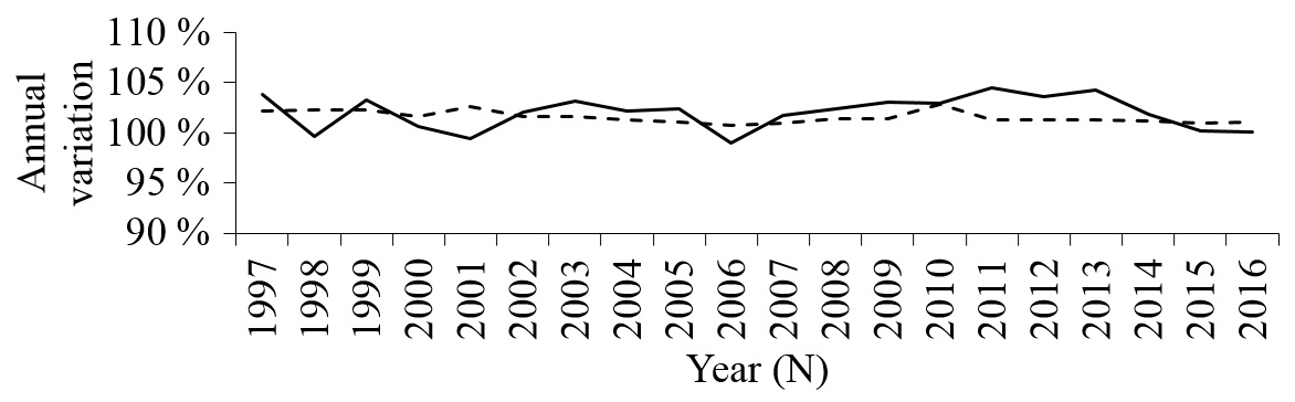
https://www.nat-hazards-earth-syst-sci.net/19/1909/2019/nhess-19-1909-2019-f03

Figure 3Comparison between the annual variations in the number of fire insurance policies for the residential line of business (solid line) and the California population (dashed line).

Download

Finally, values of P_N, t_N and W_N collected (Table 1) and estimated in this study (Eqs. 1 to 11) are aggregated into a new database presented in Table 2.

Table 2The California homeowners earthquake insurance database developed for this study. Data quality scale is as follows. A (good): all data from scientific publications with methodology explained; (B) acceptable: at least one data point from a scientific publication without details on the methodology or one processing has been applied; (C) weak: data are uncertain. Financial amounts are in 2015 US dollars. The total written premium is given in millions of US dollars. Column names are Q: data quality; E: equation ID. Abbreviations are E₁={3; 6; 7; 10} and E₂={5; 6; 7}.

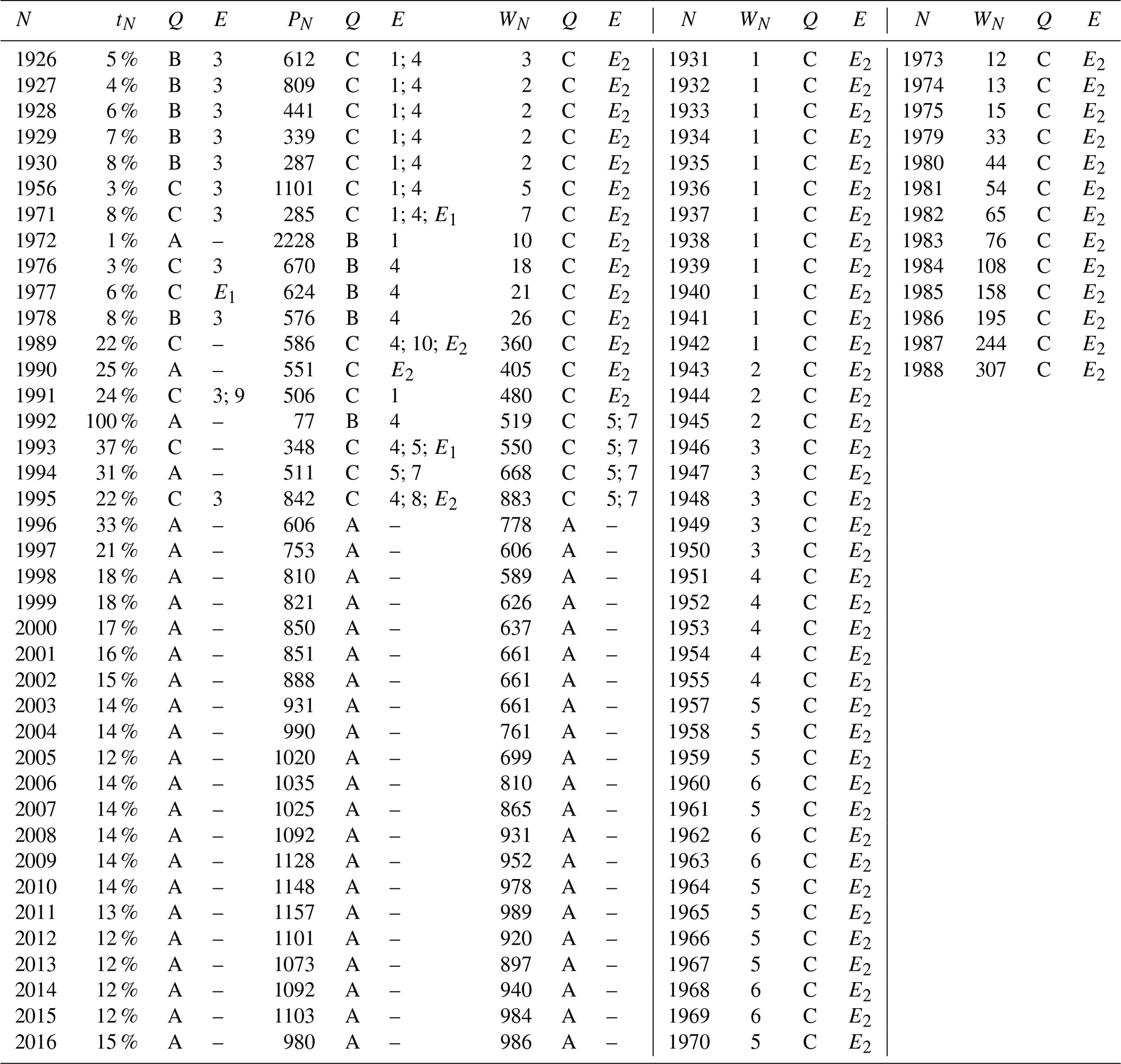
Download Print Version | Download XLSX

Financial amounts are converted into 2015 US dollars using the Consumer Price Index (US Department of Labor, 2018). The data quality of each variable is also assessed at the weakest data quality used (Table 1), by as many levels as the number of equations used to assess it (listed in the column equation ID). For example, the annual average premium P₁₉₂₆ has been calculated from the premium rate for the residential line of business $p_{1926}^{Res}$ (Table 1) and Eqs. (1) and (4). The associated data quality is C (Table 2) because the data quality of $p_{1926}^{R e s}$ is A (Table 1), downgraded by two levels for the two equations used.

The model developed in the next section uses this new database to estimate the take-up rate for the California homeowners (t_N) from the average premium amount (P_N) and another variable capturing the relative earthquake risk awareness.

3 Model development for the period 1997–2016

In order not to presume a linear trend between the consumers' behaviour and explanatory variables (e.g. the average premium amount), this study refers to the expected utility theory (Von Neumann and Morgenstern, 1944) instead of statistical linear models. The expected utility theory is a classical framework in economic science to model the economical choices of a consumer, depending on several variables like the wealth or the risk aversion (Appendix A). Here the application field is the California homeowners instead of a single consumer. Within this framework, homeowners are assumed to be rational and making decisions in order to maximize their utility. Furthermore, their relative risk aversion is considered constant whatever the wealth because the decision to purchase earthquake insurance is independent of the income level (Kunreuther et al., 1978; Wachtendorf and Sheng, 2002). One of the most used utility functions (U) is (Holt and Laury, 2002)

\begin{matrix} (12) & U (g_{N} (t_{N})) = \frac{g_{N} {(t_{N})}^{1 - β}}{1 - β}, \end{matrix}

where g_N and β are the wealth function at year N and the risk profile controlling the risk aversion level (the larger β, the higher the aversion), respectively.

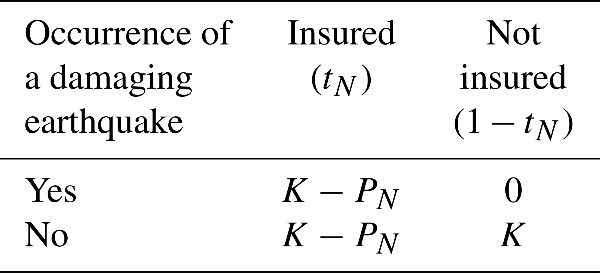
Then, the average household's capital K is assumed to be equal to the average sum insured (ASI₂₀₁₅) since the earthquake insurance consumption is uncorrelated to the wealth (Kunreuther et al., 1978; Wachtendorf and Sheng, 2002) and equal to USD 604 124 (USD 2015). Consequently, the wealth of uninsured homeowners is g_N=K, if no damaging earthquake occurs. Regarding the loss estimation, homeowners are mostly concerned by destructive earthquakes, defined as earthquakes which can potentially damage their home, and tend to overestimate the impact (Buffinton, 1961; Kunreuther et al., 1978; Meltsner, 1978; Lin, 2015). Furthermore, according to Kunreuther et al. (1978), insured people believe that they are fully covered in case of loss. Therefore, we assume that only uninsured homeowners expect to incur a loss equal to K after a damaging earthquake. This leads us to model the fact that uninsured homeowners expect a wealth at g_N=0 after a damaging earthquake. About insured homeowners, we assume that they expect to have a constant wealth at $g_{N} = K - P_{N}$ since they believe to be fully covered in case of losses induced by an earthquake. Table 3 summarizes these three wealth levels, based on the occurrence of a devastating earthquake and the insurance cover.

Table 3The four different wealth levels of a homeowner, considered in this study, according to the occurrence of a damaging earthquake and the insurance cover. The quantities t_N and 1−t_N represent the share of homeowners insured and not insured, respectively.

Download Print Version | Download XLSX

Finally, taking into account the share of insured homeowners (t_N) and the results in Table 3, g_N can be written for all homeowners as

\begin{matrix} (13) & g_{N} (t_{N}) = K - t_{N} \times P_{N} - K \times (1 - t_{N}) \times B_{EQ} (r_{N}), \end{matrix}

where ℬ_EQ(r_N) is a random variable following the Bernoulli distribution (i.e. equal to 1 if a damaging earthquake occurs during the year N and 0 otherwise). The parameter r_N, called the subjective annual occurrence probability, controls the homeowners' risk perception through the perceived probability of being affected by a destructive earthquake during the year N (Kunreuther et al., 1978; Wachtendorf and Sheng, 2002). As homeowners want to maximize their utility, t_N is solution of

\begin{matrix} (14) & t_{N}^{Estimated} = \underset{0 \leq t_{N} \leq 1}{argmax} E [U (g_{N} (t_{N}))], \end{matrix}

where argmax stands for the argument of the maxima function (i.e. which returns the value of t_N, which maximizes the quantity 𝔼[U(g_N(t_N))]) and 𝔼 is the expected value of U(g_N(t_N)), which depends on the random variable ℬ_EQ(r_N) (Eq. 13). Assuming that homeowners are risk-averse (i.e. β>0) and noticing that $\frac{P_{N}}{K}$ is very small compared to 1, $t_{N}^{Estimated}$ is shown (Appendix B) to be equal to

\begin{matrix} (15) & t_{N}^{Estimated} = \min [{(\frac{r_{N}}{1 - r_{N}} \times \frac{K}{P_{N}})}^{\frac{1}{β}}; 100 %] . \end{matrix}

As a first step, the model is calibrated with data for the period 1997–2016 corresponding to the whole activity period of the California Earthquake Authority (CEA) providing high-quality data (Table 2). Created on December 1996, this is a non-profit, state-managed organization selling residential earthquake policies (Marshall, 2017). The stability of the insurance activity and the lack of devastating earthquakes leads us to model parameters β and r_N, capturing the homeowners' risk perception, by constant variables. They are estimated at $r_{1997; \dots; 2016} = 0.027$ % and β=0.93, using the least squared method with the generalized reduced gradient algorithm. The model (Eq. 15) fits the observed data with a R²=0.79 (Fig. 4).

https://www.nat-hazards-earth-syst-sci.net/19/1909/2019/nhess-19-1909-2019-f04

Figure 4Fit between the take-up rates modelled and observed for the period 1997–2016.

Download

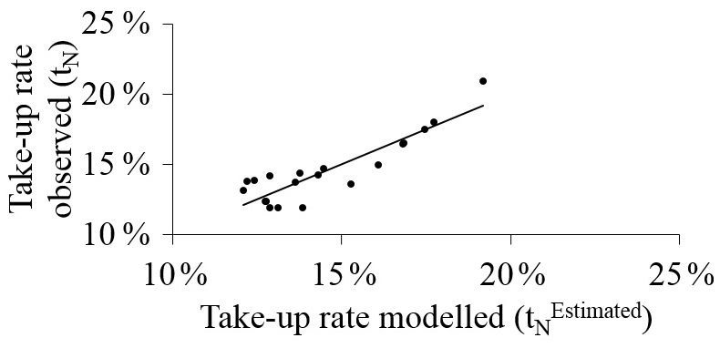
Furthermore, the values of the two parameters are meaningful: homeowners are modelled as “very risk-averse” (β=0.93), which is consistent with a high-severity risk like an earthquake (Holt and Laury, 2002). r_N is also somehow consistent with the value that can be calculated from a hazard analysis, as presented later.

The model calibration between 1997 and 2016 is not appropriate for other periods corresponding to different seismic activity and insurance economic context. The next section investigates how the homeowners' risk perception has changed since 1926 in order to adapt the model to any period.

4 Evolution of the homeowners' risk perception since 1926

The homeowners' risk perception is controlled by both the risk materiality (what kind of earthquakes are expected to occur?) and the risk tolerance (how much are homeowners ready to lose?). The associated parameters in the model are r_N and β. As we cannot differentiate the one from the other, β is assumed constant in this study and all the variations in the homeowner's risk perception are passed on to r_N.

According to the model and the relationships developed (Eqs. 3–5, 10–11 and 15), the variations in the total written premium amount per capita (W_N∕Pop_N) depend on the variation in the average premium amount (P_N) and the subjective annual occurrence probability (r_N):

\begin{matrix} (16) & \begin{aligned} \frac{W_{N} / {Pop}_{N}}{W_{N - 1} / {Pop}_{N - 1}} & = \frac{Δ_{W_{N - 1}}^{W_{N}^{Res}}}{Δ_{{Pop}_{N - 1}}^{{Pop}_{N}}} \\ = Δ_{P_{N - 1}}^{P_{N}} \times Δ_{t_{N - 1}}^{t_{N}} \\ = Δ_{P_{N - 1}}^{P_{N}} \times \frac{\min [{(\frac{r_{N}}{1 - r_{N}} \times \frac{K}{P_{N}})}^{\frac{1}{β}}; 100 %]}{\min [{(\frac{r_{N - 1}}{1 - r_{N - 1}} \times \frac{K}{P_{N - 1}})}^{\frac{1}{β}}; 100 %]} . \end{aligned} \end{matrix}

Under the assumption that $t_{N}^{Estimated}$ has never reached 100 % in the past and with β=0.93, Eq. (16) can be simplified as follows:

\begin{matrix} (17) & \begin{aligned} \frac{W_{N} / {Pop}_{N}}{W_{N - 1} / {Pop}_{N - 1}} & = Δ_{P_{N - 1}}^{P_{N}} \times \frac{{(\frac{r_{N}}{1 - r_{N}} \times \frac{K}{P_{N}})}^{\frac{1}{β}}}{{(\frac{r_{N - 1}}{1 - r_{N - 1}} \times \frac{K}{P_{N - 1}})}^{\frac{1}{β}}} \\ = {(\frac{P_{N}}{P_{N - 1}})}^{- 0.07} \times {(\frac{r_{N} \times (1 - r_{N - 1})}{r_{N - 1} \times (1 - r_{N})})}^{1.07} . \end{aligned} \end{matrix}

The contribution of $P_{N} / P_{N - 1}$ is clearly marginal, leading to consider the regression, built on the variations in W_N∕Pop_N and r_N between 1997 and 2016 (Table 2):

\begin{matrix} (18) & \frac{r_{N}}{r_{N - 1}} - 1 = 0.92 \times (\frac{W_{N} / {Pop}_{N}}{W_{N - 1} / {Pop}_{N - 1}} - 1) (R^{2} = 1) . \end{matrix}

Equations (16) and (18) used and the goodness of fit are illustrated in Fig. 5a and b, respectively.

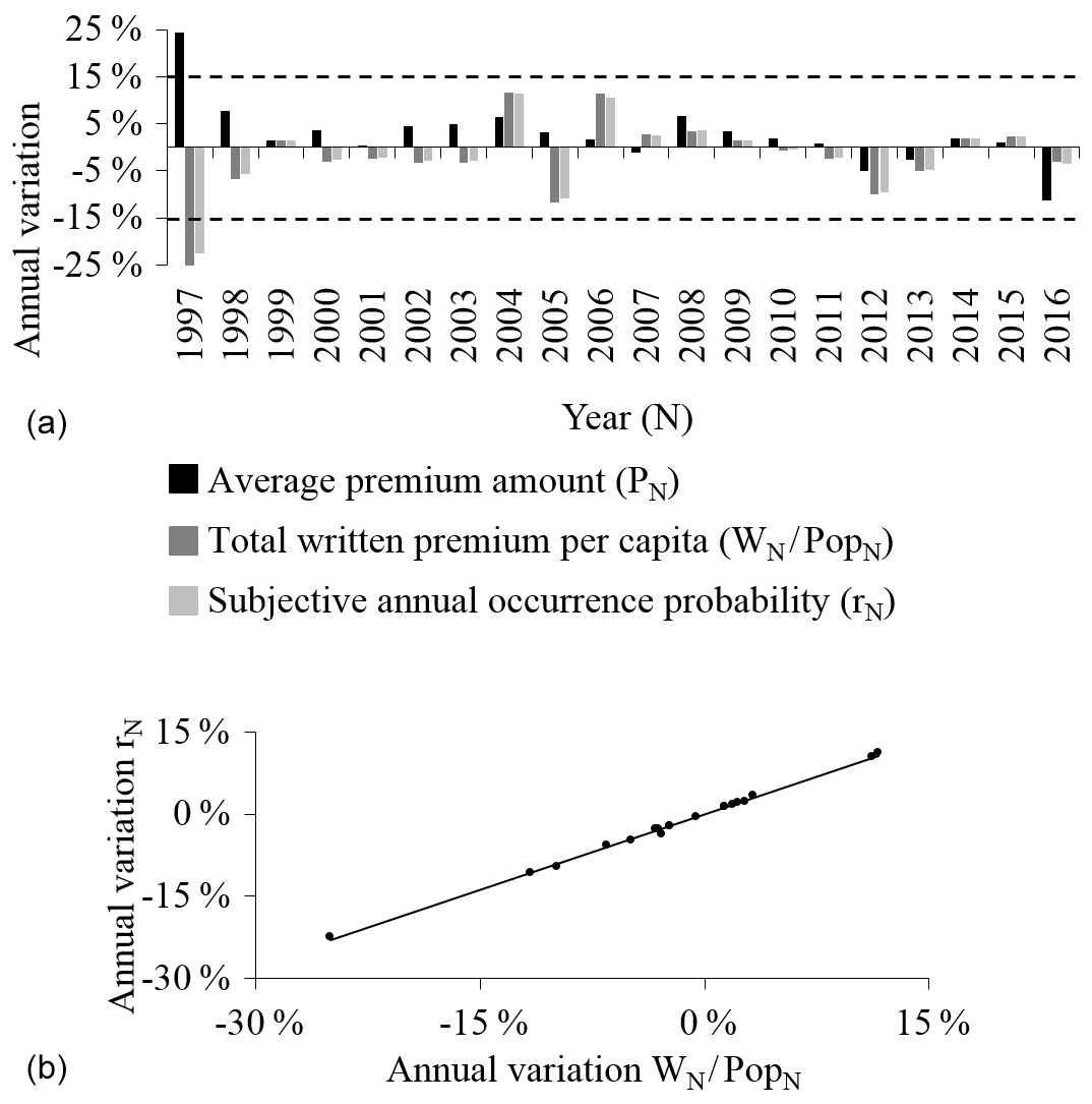
https://www.nat-hazards-earth-syst-sci.net/19/1909/2019/nhess-19-1909-2019-f05

Figure 5(a) Variations in the average premium amount, the total written premium per capita and the subjective annual occurrence probability between 1997 and 2016. Variations are calculated compared to the previous year. Dashed lines represent the thresholds for a significant variation. (b) Fit between the variation in the total written premium per capita and the subjective annual occurrence probability.

Download

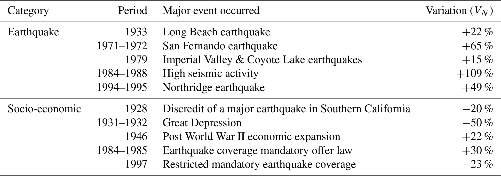
Considering that understanding the details of those variations is out of reach given the scarcity of data, this study focuses only on those above 15.5 % in absolute value, qualified hereafter as significant variations (V_N). Other variations are neglected and we assume they cancel each other out. Table 4 lists all of them, together with the most significant event that occurred the same year, for the earthquake insurance industry. Despite the fact that these events (Table 4) could have led insurance companies to restrict or enlarge the number of earthquake insurance policies (Born and Klimaszewski-Blettner, 2013), contributing in this way to V_N, this study focuses only on the homeowners' risk perception variations.

Table 4Events expected to have significantly modified the homeowners' risk perception through the subjective annual occurrence probability. V_N represents the variation compared to the previous year, with the sign “+” for an increase and “−” for a decrease.

Download Print Version | Download XLSX

Then, the subjective annual occurrence probability (r_N) is estimated according to the following time series for N∈[1926; 2016]:

\begin{matrix} (19) & \{\begin{cases} r_{2016} & = 0.027 % \\ r_{N} & = \frac{r_{N + 1}}{1 + V_{N + 1}} \forall N \in [1926; 2015] \end{cases} . \end{matrix}

The time series of r_N is represented in Fig. 6 and illustrates that some earthquakes (indicated by dots) have increased r_N during the year as already published (Buffinton, 1961; Kunreuther et al., 1978; Meltsner, 1978; Lin, 2015), but, more surprisingly, some others had no apparent impact, like the 1952 Kern County and 1989 Loma Prieta earthquakes.

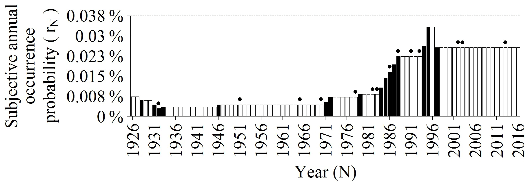
https://www.nat-hazards-earth-syst-sci.net/19/1909/2019/nhess-19-1909-2019-f06

Figure 6Estimated subjective annual occurrence probability between 1927 and 2016. The horizontal dashed line corresponds to the historical average value. Black bars represent the significant evolutions and dots indicate the occurrence of the following big earthquakes in California: 1933 Long Beach, 1952 Kern County, 1966 Parkfield, 1971 San Fernando, 1979 Coyote Lake, 1979 Imperial Valley and Coyote Lake, 1983 Coalinga, 1984 Morgan Hill, 1987 Whittier Narrows, 1989 Loma Prieta, 1992 Big Bear and Landers, 1994 Northridge, 2003 San Simeon, 2004 Parkfield and 2014 Napa.

Download

The first earthquake damaged over 400 unreinforced masonry buildings (Jones et al., 2012), but none of the buildings were designed under the latest seismic codes (Geschwind, 2001). Consequently, structural engineers claimed that new buildings were earthquake-proof and that no additional prevention measures were needed (Geschwind, 2001). This message was received well among the population despite the warnings of some earthquake researchers like Charles Richter (Geschwind, 2001).

Regarding the second earthquake, most homeowners were only partially refunded, due to large deductibles, and decided to cancel their earthquake insurance policies (Meltsner, 1978; Palm and Hodgson, 1992b; Burnett and Burnett, 2009). Moreover, the 1989 Loma Prieta earthquake struck just after a high-seismic-activity period during which r_N increased significantly. Indeed, the number of earthquakes occurring during the preceding 5 years with a moment magnitude greater than M5 reached the highest peak since 1855 between 1984 and 1998, as illustrated in Fig. 7.

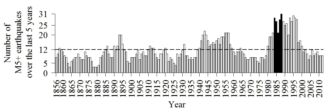
https://www.nat-hazards-earth-syst-sci.net/19/1909/2019/nhess-19-1909-2019-f07

Figure 7Number of earthquakes with a moment magnitude M5+ occurring during the 5 previous years. For year N, the sum is calculated from N−5 to N−1. Earthquakes occurring the same day count as one. Black bars correspond to the peak of seismicity observed between 1984 and 1988. The dotted line represents the average value from 1855 to 2012. The historical earthquake database used is taken from the UCERF3 (Field et al., 2013; Felzer, 2013).

Download

The sequence includes in particular the 1983 Coalinga and the 1987 Whittier Narrows earthquakes. This specific temporal burst in seismic activity may have contributed to homeowners' rising risk awareness (Table 4).

Some major socio-economic events also had an impact on r_N (Table 4), such as the 1929 Great Depression and the post World War II economic expansion. Insurance regulation acts also have an impact. During the period 1984–1985, the California senate assembly voted on the Assembly Bill AB2865 (McAlister, 1984), which required insurance companies to offer earthquake coverage. A second bill in 1995, named AB1366 (Knowles, 1995), amended the Insurance Code Section 10089 to restrict the extent of the mandatory cover and addressed the insurance crisis caused by the 1994 Northridge earthquake. The new “mini-policy” met with limited success mainly because the price was more expensive for a lower guarantee (Reich, 1996). Furthermore, the creation of the CEA was at odds with the trend in insurance market privatization and people perceived it as an insurance industry bailout (Reich, 1996). The combined impact on r_N of the two assembly bills is null as (1+30 %) × (1−23 %) = 1 (Table 4). It means that the efforts to promote earthquake insurance among the population by a first assembly bill were cancelled 20 years later by the other. Last, the discredit of a mistaken prediction can lead to a decrease in r_N, as happened in 1928 with the occurrence of a major earthquake in Southern California (Geschwind, 1997; Yeats, 2001).

r_N is then compared to a scientifically based earthquake annual occurrence probability to assess the level of the homeowners' risk perception. This requires the assessment of the annual probability for a homeowner of being affected by a destructive earthquake. For that, the ShakeMap footprints, released by the US Geological Survey (Allen et al., 2009), are used. A ShakeMap footprint gives, for a historical earthquake, the modelled ground motions for several metrics, including the macroseismic intensity on the modified Mercalli intensity scale (MMI). In California, a total of 564 ShakeMap footprints are available on the USGS website (https://earthquake.usgs.gov/data/shakemap/) for the period 1952–2018 and the magnitude range M3–M7.3. According to the MMI scale, heavy damage can be observed for an intensity above or equal to VIII. Among the 564 historical earthquakes, the ShakeMap footprints report that only 21 have caused such a high intensity and are labelled as destructive earthquakes. For each of the 21 ShakeMap footprints, the area corresponding to an intensity above or equal to VIII was reported in Table 5 and the population living inside was estimated using the Global Settlement Population Grid (European Commission; Florczyk et al., 2019).

Table 5Earthquakes that have occurred in California since 1950 with a maximum macroseismic intensity on the modified Mercalli scale (MMI) modelled by the ShakeMap programme (US Geological Survey) above or equal to VIII. The columns “area” and “number of people affected” give the size and the estimated population of the area affected above or equal to VIII, respectively. The population has been assessed using the Global Human Settlement Population Grid (European Commission, Florczyk et al., 2019).

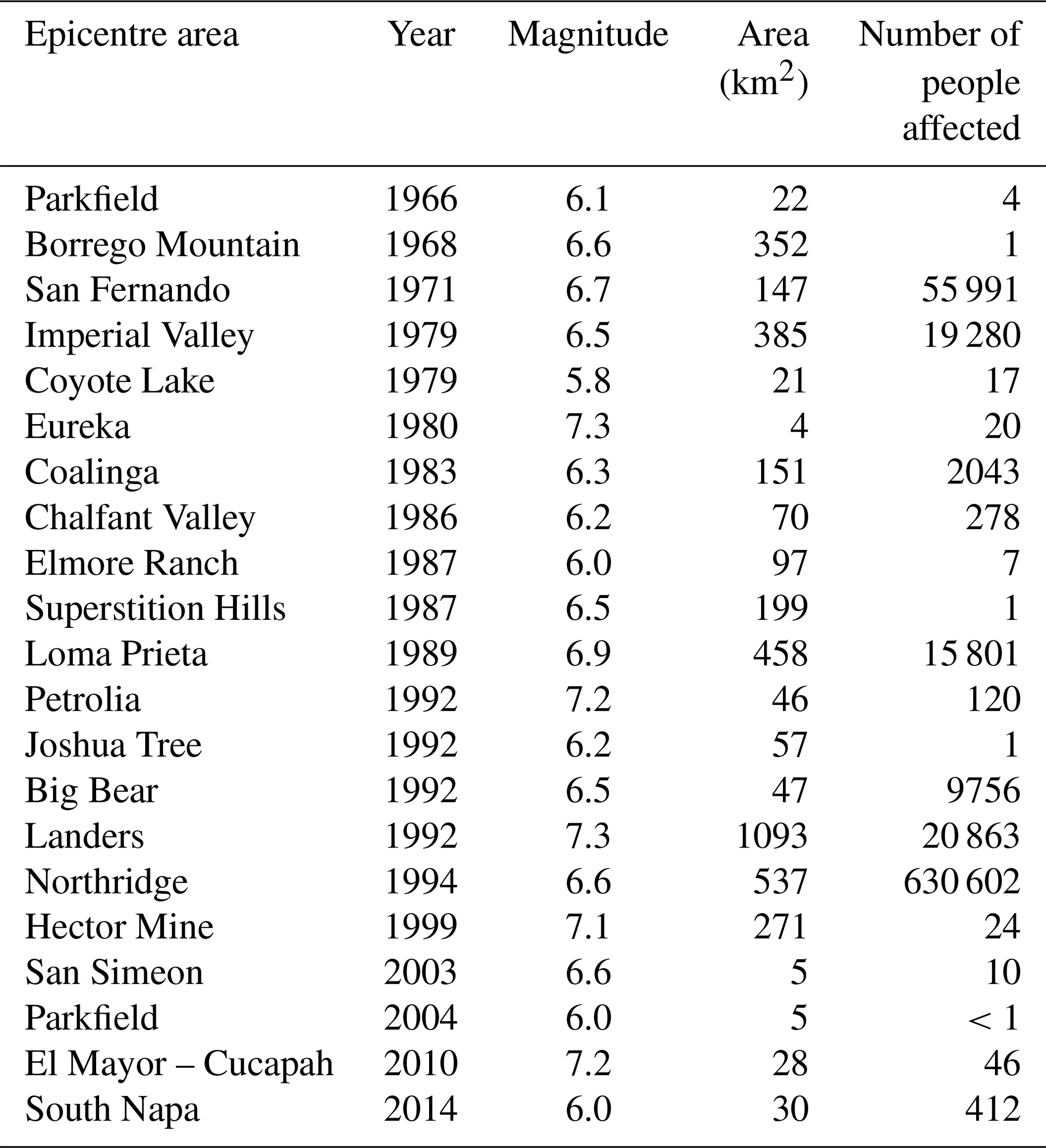
Download Print Version | Download XLSX

Finally, for each year since 1952, the annual rate of people was calculated by dividing the number of people having experienced an intensity above or equal to VIII by the total population of California according to the Global Human Settlement Population Grid (European Commission, Florczyk et al., 2019). The arithmetic mean of the annual rates during the period 1952–2018 is equal to r^Hist=0.038 %. In this study, we consider r^Hist as the true average probability for a California homeowner to be affected by a destructive earthquake. Therefore, the risk has always been underestimated by California homeowners because AWR_N has been lower than r^Hist since 1926 (Fig. 6). The severity underestimation is quantified using the earthquake risk awareness ratio (AWR_N) defined as

\begin{matrix} (20) & {AWR}_{N} = \frac{r_{N}}{r^{Hist}} = 2632 \times r_{N} . \end{matrix}

With AWR_N being estimated since 1926, the take-up rate model is generalized in the next section and used to understand the current low take-up rate.

5 Understanding the current low take-up rate

Introducing the earthquake risk awareness ratio (AWR_N), we redefine the take-up rate model (Eq. 15) as follows:

\begin{matrix} (21) & t_{N}^{Estimated} = \min [{(\frac{{AWR}_{N}}{2632 - {AWR}_{N}} \times \frac{K}{P_{N}})}^{1.07}; 100 %] . \end{matrix}

From the estimated values of AWR_N (Eqs. 19 and 20) and P_N (Table 2), Fig. 8 shows the fit between $t_{N}^{Estimated}$ (Eq. 21) and t_N (Table 2).

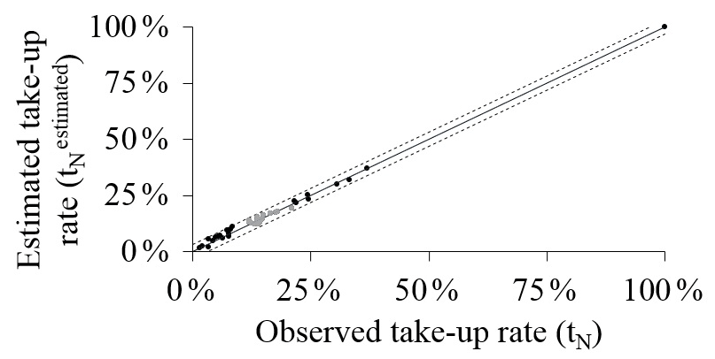
https://www.nat-hazards-earth-syst-sci.net/19/1909/2019/nhess-19-1909-2019-f08

Figure 8Comparison between the take-up rates observed and estimated using the model developed in this study. Grey points correspond to the period 1997–2016, which was used to calibrate the model. Dashed lines represent a buffer of ±0.03.

Download

The goodness of fit is R²=0.99 and the modelling errors are below ±3 %, as represented by the dashed lines. The record at 100 % corresponds to the 1992 California Residential Earthquake Recovery Fund Program (CRER), which was a mandatory public earthquake insurance, including a cover amount for households up to USD 15 000 (USD 1992), at a very low premium amount (Lagorio et al., 1992).

Figure 9 illustrates the sensitivity of $t_{N}^{Estimated}$ to the average premium P_N and the earthquake risk awareness ratio AWR_N (Eq. 20).

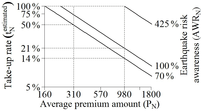
https://www.nat-hazards-earth-syst-sci.net/19/1909/2019/nhess-19-1909-2019-f09

Figure 9Relationship between the average premium amount, the take-up rate and the earthquake risk awareness. Financial values are in US dollars (2015).

Download

The lines AWR_N=70 %, AWR_N=100 % and AWR_N=425 % stand for the current situation, the true risk level and the target value of AWR_N for $t_{N}^{Estimated} = 100$ %, at the current price of USD 980 (USD 2015), respectively. According to the first value (AWR_N=70 %), half of homeowners ( $t_{N}^{Estimated} = 50$ %) are not willing to pay an average premium amount exceeding P_N = USD 310 (USD 2015) per year for an insurance cover. This would represent a 68 % decrease in the price of earthquake insurance coverage.

Conversely, the relatively low earthquake risk awareness (AWR_N=70 %) contributes only marginally to the current low take-up rate ( $t_{N}^{Estimated} = 14$ %). In fact, even with the true level of risk (AWR_N=100 %), only $t_{N}^{Estimated} = 21$ % of homeowners are expected to buy insurance. This result is consistent with previous findings by Shenhar et al. (2015), who observed in Israel that the earthquake insurance take-up rate did not significantly increase after a large prevention campaign.

To reach a 100 % take-up rate with the current premium amount, according to the model, the earthquake risk awareness ratio has to reach 425 %, which is very unlikely. Indeed, the UCERF3 assesses the annual probability of occurrence, in California, of an earthquake with a magnitude above M6.7 at 15 % (Field et al., 2013). Under the assumption that the probability for a homeowner of experiencing a damaging earthquake is proportional to the occurrence of such an earthquake, reaching that awareness ratio would mean that homeowners consider this probability to reach the level of 425 % × 15 % = 64 %. In other words, only the belief that a destructive earthquake is imminent (i.e. a probability of occurrence somewhere in California during the year, for a 1994 Northridge-like earthquake, above 64 %) can bring all homeowners to buy an earthquake insurance plan at the current price.

6 Conclusions

The model developed in the present study shows that the low earthquake insurance take-up rate, observed until 2016 for the homeowner line of business in California, is due foremost to high premiums. Indeed, no homeowner would prefer to stay uninsured against earthquake risk if the annual average premium were to decrease from USD 980 (as observed in 2016) to USD 160 (USD 2015) or lower. Moreover, Kovacevic and Pflug (2011) have shown that a minimum capital is required to benefit from an earthquake insurance cover, otherwise the cost of the premium would be more than the potential risk. They have also found that the lower the insurance premium, the lower this minimum capital. Consequently, the results of Kovacevic and Pflug (2011) suggest that some uninsured people can be well aware of the earthquake risk but just cannot afford earthquake insurance at the current price. This corroborates the result of the present study because bringing such people to buy earthquake insurance is foremost a matter of price, not of insufficient risk perception.

Nevertheless, as the current average premium amount corresponds to the annualized risk assessment, insurance companies would not have enough reserves to pay future claims following earthquakes if they collect on average only USD 160 per policy (CEA, 2017). Hence, the current insurance mechanism cannot meet the homeowners' demand and be sustainable, as was the case for the 1992 CRER programme (Kunreuther et al., 1998).

Since this initiative, earthquake insurance has not been mandatory in California. Because compulsory insurance is not only hard to implement but also has an unpredictable impact (Chen and Chen, 2013), new insurance solutions have emerged to increase the earthquake insurance market, like parametric insurance. This insurance product stands out from traditional insurance policies by paying a fixed amount when the underlying metrics (e.g. the magnitude and the epicentre location) exceed a threshold, whatever the loss incurred by the policyholder. This new insurance claim process significantly reduces the loss uncertainty, the operating expenses and so the premium rate. In California, parametric insurance has been offered to cover homeowners against earthquake risk since 2016 (Jergler, 2017).

Nevertheless, risk awareness remains important in earthquake insurance consumption, and insurance companies also encourage local policies led by public authorities to improve prevention (Thevenin et al., 2018).

This study supports these initiatives by demonstrating that a new earthquake insurance scheme is necessary to meet the premium expected by homeowners. However, it also shows that the lower the premium amount, the more the earthquake risk awareness contributes in insurance consumption (Fig. 9). Finally, only a global effort involving all stakeholders may fill the adoption gap in earthquake insurance coverage. This also includes the financial stakeholders, involved in the mortgage loan business. A recent study (Laux et al., 2016) analysed the fact that most banks do not require earthquake insurance from their mortgage loan clients, preferring instead to keep the risk and to increase the interest rate by +0.2 % (in 2013). These additional bank fees are, on average, as expensive as the premium rate for the residential earthquake insurance (0.185 % in 2013 according to the CDI, 2017a). Nevertheless, such a market practice puts an estimated USD 50 billion–100 billion loss risk on the US mortgage system (Fuller and Kang, 2018). Consequently, expanding earthquake insurance cover, for homeowners, is also a challenge for the banking industry. In this respect, requiring earthquake insurance for mortgage loans would strongly enhance the insurance and public initiatives.

Data availability

Insurance market raw data and socio-economic indicators collected between 1921 and 2016 in California are available in the Supplement.

Appendix A: The expected utility theory

The expected utility theory (also called the von Neumann–Morgenstern utilities) was introduced in 1947 by von Neumann and Morgenstern. It models a decision maker's preferences from a basket of goods (materialized by the function g), according to their utility. Under this framework, the utility is defined as the satisfaction that a decision maker receives from the goods they get. The utility is measured by a utility function, U_i, where i is the name of the decision maker. The function U_i is defined by the Von Neumann and Morgenstern (1944) theorem, which is based on several axioms that could be split in six parts (Narahary, 2012). For the first two, let us consider a basket of three goods: b={g₁; g₂:g₃}. Then, the two first axioms state the following.

Completeness. The decision maker can always compare two goods (e.g. g₁ and g₂) and decide which one they prefer or if both are equal.
Transitivity. If the decision maker prefers g₁ to g₂ and g₂ to g₃, then they also prefer g₁ to g₃.

Let us now consider that the decision maker does not select a good from a basket of goods b={g₁; g₃} but instead participates in a lottery l₁ on b. We introduce p₁ and 1−p₁ as the probability for the decision maker to win the goods g₁ and g₃, respectively. Similarly, l₂ is the lottery on b with the probabilities p₂ and 1−p₂. Here, the decision maker can choose between two different lotteries. On this basis, the four remaining axioms are as follows.

3.
Substitutability. The decision maker has no preference between l₁ and the same lottery where g₁ is changed by g₄ if the decision maker has no preference between g₁ and g₄.
4.
Decomposability. The decision maker has no preference on the way to carry on the lottery l₁, as long as long as the probabilities (p₁ and 1−p₁) remain the same.
5.
Monotonicity. Between l₁ and l₂, the decision maker always prefers the one with the higher chance of winning their favourite good (i.e. if they prefer g₁ to g₃, then the decision maker prefers l₁ to l₂ when p₁>p₂, and reciprocally).
6.
Continuity. If the decision maker prefers g₁ to g₂ and g₂ to g₃, there is a value of p₁ for which the decision maker has no preference between having g₂ and participating at l₁.

According to the von Neumann–Morgenstern theorem, a utility function associates a good g₁ with a level of utility U_i(g₁) for the decision maker i. When the good g₁ is replaced by a lottery l₁, this theorem states that the level of utility is the weighted average: $U_{i} (l_{1}) = p_{1} \times U_{i} (g_{1}) + (1 - p_{1}) \times U_{i} (g_{3})$ .

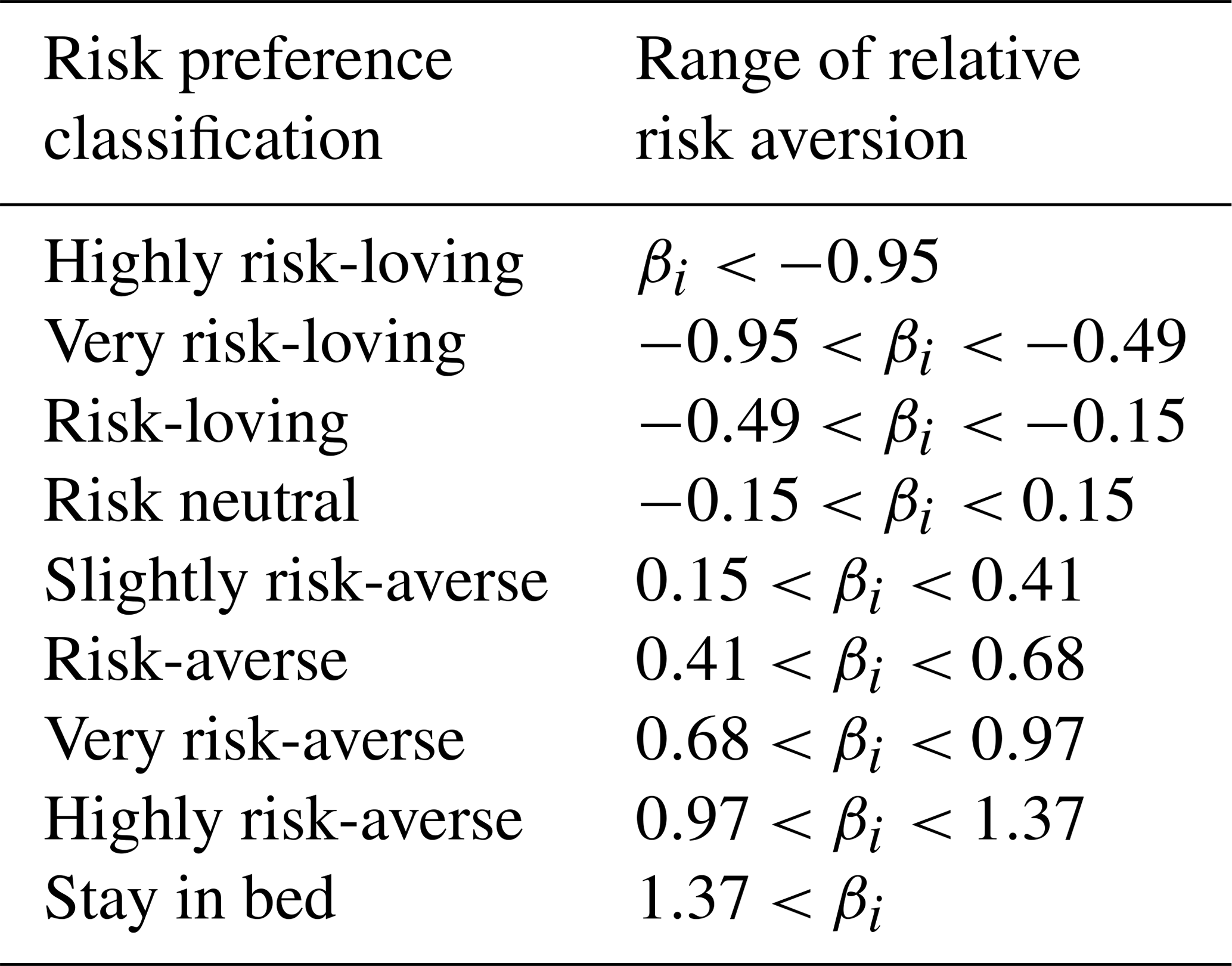
Table A1Risk preference scale depending on the parameter β_i, according to Holt and Laury (2002).

Download Print Version | Download XLSX

The first property of U_i is to be strictly increasing (i.e. its first derivative $U_{i}^{'}$ is strictly positive). When g₁ corresponds to the decision maker's wealth, like in this study, it means that the decision maker always wants to increase their level of wealth. Conversely, the sign of the second derivative, $U_{i}^{''}$ , can be positive (i.e. U_i is convex) or negative (i.e. U_i is concave). It represents the decision maker's behaviour: when $U_{i}^{''} < 0$ , the decision maker is risk-averse, meaning that the difference of utility between g₁ and g₁+1 is decreasing when g₁ increases. Still considering that g₁ is the decision maker's wealth, it means that increasing the wealth by EUR +100 provides a higher utility for a decision maker with a wealth g₁ = EUR 1000 than for one with a wealth g₁ = EUR 1 000 000. In terms of insurance, a risk-averse decision maker wants to be covered. Indeed, we assume that the decision maker can be protected against losing g₁ with a probability p₁ when paying a premium amount $P_{N} = p_{1} \times g_{1}$ . Since the utility function is concave, the following equation is verified:

\begin{matrix} (A1) & U_{i} (0) \times p_{1} + U_{i} (g_{1}) \times (1 - p_{1}) < U_{i} (g_{1} - P_{N}) . \end{matrix}

Conversely, when $U_{i}^{''} > 0$ , the decision maker is risk-loving and behaves in the opposite way.

Depending on the choice of U_i, this behaviour (risk-averse or risk-loving) can change depending on g₁. To represent it, the Arrow–Pratt measure of relative risk aversion (named after Pratt, 1964, and Arrow, 1965) is used:

\begin{matrix} (A2) & RRA (g_{1}) = g_{1} \times \frac{- U_{i}^{''} (g_{1})}{U_{i}^{'} (g_{1})} . \end{matrix}

When RRA, the Arrow–Pratt measure of relative risk aversion, is decreasing, increasing or constant, it means that the decision maker is less, more or indifferently risk-averse with the value of the good g₁.

The utility function U_i used in this study was developed by Holt and Laury (2002).

\begin{matrix} (A3) & U_{i} (g_{1}) = \{\begin{cases} \frac{g^{1 - β_{i}}}{1 - β_{i}} & if β_{i} \neq 1 \\ \log (g_{1}) & otherwise, \end{cases} \end{matrix}

where β_i is the level of relative risk aversion and materializes the decision maker's risk behaviour from highly risk-loving to highly risk-averse. Indeed, one can verify that the RRA measure for the Holt and Laury (2002) utility function is RRA(g₁)=β_i. Therefore, this function belongs to the constant risk relative aversion utility function family. It means that a decision maker's behaviour is assumed to be uncorrelated to their wealth level (g₁). Furthermore, the parameter β_i controls the decision maker's behaviour (Table A1).

Appendix B: Solution of the expected utility maximization equation

Let us consider the following mathematical problem in Eq. (B1):

\begin{matrix} (B1) & t_{N}^{Estimated} = \underset{0 \leq t_{N} \leq 1}{} argmax E [U (g_{N} (t_{N}))] . \end{matrix}

The function f(t_N)=𝔼[U(g_N(t_N))] can be rewritten by detailing the expression of the expected utility 𝔼:

\begin{matrix} (B2a) & \begin{aligned} f (t_{N}) & = U (g_{N} (t_{N})) \times P (B_{E Q} (r_{N}) = 0) \\ + U (g_{N} (t_{N})) \times P (B_{E Q} (r_{N}) = 1) . \end{aligned} \end{matrix}

Introducing the definition of g_N(t_N) (Eq. A3) gives

\begin{matrix} (B2b) & \begin{aligned} f (t_{N}) & = U (K - t_{N} \times P_{N}) \times P (B_{E Q} (r_{N}) = 0) \\ + U (K - t_{N} \times P_{N} - K \times (1 - t_{N})) \\ \times P (B_{E Q} (r_{N}) = 1) . \end{aligned} \end{matrix}

Using the definition of the function U (Eq. A2), f(t_N) becomes

\begin{matrix} (B2c) & \begin{aligned} f (t_{N}) & = (\frac{{(K - t_{N} \times P_{N})}^{1 - β}}{1 - β}) P (B_{E Q} (r_{N}) = 0) \\ + (\frac{{(t_{N} \times (K - P_{N}))}^{1 - β}}{1 - β}) P (B_{E Q} (r_{N}) = 1) \\ = \frac{1}{1 - β} [(1 - r_{N}) {(K - t_{N} \times P_{N})}^{1 - β} \\ + r_{N} {(K - P_{N})}^{1 - β} t_{N}^{1 - β}] . \end{aligned} \end{matrix}

Furthermore, the derivative of f(t_N) is equal to

\begin{matrix} (B2d) & \{\begin{cases} \frac{δ f (t)}{δ t_{N}} & = (- P_{N}) (1 - r_{N}) {(K - t_{N} \times P_{N})}^{- β} \\ + r_{N} {(K - P_{N})}^{1 - β} t_{N}^{- β} \\ \frac{δ f (0)}{δ t_{N}} & = + \infty \\ \frac{δ f (1)}{δ t_{N}} & = {(K - P_{N})}^{- β} (K r_{N} - P_{N}) \end{cases} . \end{matrix}

Thus, when $\frac{δ f (1)}{δ t_{N}} < 0$ , $t_{N}^{Estimated}$ is equal to (otherwise, $t_{N}^{Estimated} = 1$ )

\begin{matrix} (B2e) & \begin{aligned} \frac{δ f (t_{N}^{Estimated})}{δ t} = 0 & \Leftrightarrow {(\frac{K}{t_{N}^{Estimated}} - P_{N})}^{- β} \times P_{N} \\ \times (1 - r_{N}) = r_{N} \times {(K - P_{N})}^{1 - β} \\ \Leftrightarrow t_{N}^{Estimated} = \frac{K X}{K - P_{N} + P_{N} X} \\ where X = {(\frac{r_{N} (K - P_{N})}{P_{N} (1 - r_{N})})}^{\frac{1}{β}} . \end{aligned} \end{matrix}

As the expression of $t_{N}^{Estimated}$ is complex, it can be simplified using the approximation $\frac{P_{N}}{K} \approx 0$ :

\begin{matrix} (B2f) & \begin{array}{ll} t_{N}^{Estimated} & = X \\ = {(\frac{r_{N} (K - P_{N})}{P_{N} (1 - r_{N})})}^{\frac{1}{β}} \\ = {(\frac{r_{N}}{(1 - r_{N})} \times \frac{K}{P_{N}})}^{\frac{1}{β}} \times {(1 - \frac{P_{N}}{K})}^{\frac{1}{β}} \\ = {(\frac{r_{N}}{(1 - r_{N})} \times \frac{K}{P_{N}})}^{\frac{1}{β}} . \end{array} \end{matrix}

Supplement

The supplement related to this article is available online at: https://doi.org/10.5194/nhess-19-1909-2019-supplement.

Author contributions

AP had a role in the following in this study: conceptualization, formal analysis, investigation, methodology and writing. PG performed the supervision, validation, and visualization and also wrote the original draft. PYB and SB were involved in the validation as well as in the writing, review and editing processes.

Competing interests

The authors declare that they have no conflict of interest.

Acknowledgements

The authors acknowledge Madeleine-Sophie Déroche, CAT Modelling R & D Leader at AXA Group Risk Management, for her contribution to this work. They are also grateful to the California Department of Insurance, the EM-DAT, Robert Shiller, the US Census, the US Department of Labor, and the USGS for providing open access to their databases.

Financial support

This research has been supported by the European Union's H2020 Research and Innovation programme under the Marie Skłodowska-Curie grant (grant no. 813137) and Labex OSUG@2020 (Investissements d'avenir, ANR10-LABX56 grant).

Review statement

This paper was edited by Sven Fuchs and reviewed by two anonymous referees.

References

Allen, T. I., Wald, D. J., Earle, P. S., Marano, K. D., Hotovec, A. J., Lin, K., and Hearne, M. G.: An Atlas of ShakeMaps and population exposure catalog for earthquake loss modeling, Bull. Earthquake Eng., 7, 701–718, 2009.

Arrow, K. J.: Aspects of the Theory of Risk Bearing, in: The Theory of Risk Aversion, Yrjo Jahnssonin Saatio, Helsinki, 1965.

Asprone, D., Jalayer, F., Simonelli, S., Acconcia, A., Prota, A., and Manfredi, G.: Seismic insurance model for the Italian residential building stock, Struct. Saf., 44, 70–79, 2013.

Born, P. H. and Klimaszewski-Blettner, B. K.: Should I Stay or Should I Go? The Impact of Natural Disasters and Regulation on U.S. Property Insurers' Supply Decisions, J. Risk. Insur., 80, 1–36, 2019.

Buffinton, P.: Earthquake Insurance In The United States – A Reappraisal, Bull. Seismol. Soc. Am., 51, 315–329, 1961.

Burnett, B. and Burnett, K.: Is Quake Insurance Worth it?, SFGate, available at: https://www.sfgate.com/homeandgarden/article/Is-quake-insurance-worth-it-3246888.php (last access: 12 January 2018), 25 March 2009.

California Earthquake Authority: Our Financial Strength – More than $15 billion in claim-paying capacity, available at: https://www.earthquakeauthority.com/who-we-are/cea-financial-strength (last access: 12 January 2018), 2017.

CDI – California Department of Insurance: Residential and Earthquake Insurance Coverage Study, CA EQ Premium, Exposure, and Policy Count Data Call Summary, available at: http://www.insurance.ca.gov/0400-news/0200-studies-reports/0300-earthquake-study/ (last access: 19 December 2017), 2017a.

CDI – California Department of Insurance: California Insurance Market Share Reports, available at: http://www.insurance.ca.gov/01-consumers/120-company/04-mrktshare/ (last access: 17 December 2017), 2017b.

CDI – California Department of Insurance: Information Guides, Earthquake Insurance, available at: http://www.insurance.ca.gov/01-consumers/105-type/95-guides/03-res/eq-ins.cfm, last access: 2 July 2019.

Chen, Y. and Chen, D.: The review and analysis of compulsory insurance, Insurance Markets and Companies: Analyses and Actuarial Computations, Business Perspectives, Ukraine, 4, 1, 2013.

Eguchi, R., Goltz, J., Taylor, C., Chang, S., Flores, P., Johnson, L., Seligson, H., and Blais, N.: Direct Economic Losses in the Northridge Earthquake: A Three-Year Post-Event Perspective, Earthq. Spectra, 14, 245–264, 1998.

Florczyk, A. J., Corbane, C., Ehrlich, D., Freire, S., Kemper, T., Maffenini, L., Melchiorri, M., Pesaresi, M., Politis, P., Schiavina, M., Sabo, F., and Zanchetta, L.: GHSL Data Package 2019, EUR 29788 EN, JRC 117104, Publications Office of the European Union, Luxembourg, 2019.

Felzer, K. R.: UCERF3, Appendix K: The UCERF3 Earthquake Catalog, available at: https://pubs.usgs.gov/of/2013/1165/data/ofr2013-1165_EarthquakeCat.txt (last access: 27 November 2018), 2013.

Field, E., Biasi, G., Bird, P., Dawson, T., Felzer, K., Jackson, D., Johnson, K., Jordan, T., Madden, C., Michael, A., Milner, K., Page, M., Parsons, T., Powers, P., Shaw, B., Thatcher, W., Weldon, R., and Zeng, Y.: Uniform California earthquake rupture forecast, version 3 (UCERF3) – The time-independent model, US Geological Survey Open-File Report 2013-1165, California Geological Survey Special Report 228, and Southern California Earthquake Center Publication 1792, p. 97, 2013.

Freeman, J.: Earthquake Damage And Earthquake Insurance, 1st Edn., Mc Graw-Hill Book Company Inc., New York, London, 1932.

Fuller, T. and Kang, I.: California Today: Who Owns the Risk for Earthquakes?, New York Times, available at: https://www.nytimes.com/2018/09/11/us/california-today-earthquake-insurance.html (last access: 3 December 2018), 11 September 2018.

Garamendi, J., Roth, R., Sam, S., and Van, T.: California Earthquake Zoning And Probable Maximum Loss Evaluation Program: An Annual Estimate Of Potential Insured Earthquake Losses From Analysis Of Data Submitted By Property And Casualty Companies In California, Diane Pub Co, California Department of Insurance, Los Angeles, California, 1992.

Garrat, R. and Marshall, J. M.: Equity Risk, Conversion Risk, And The Demand For Insurance, J. Risk. Insur., 70, 439–460, 2003.

Geschwind, C.: 1920s Prediction Reveals Some Pitfalls of Earthquake Forecasting, Eos, 78, 401–412, 1997.

Geschwind, C.: California Earthquakes: Science, Risk & the Politics of Hazard Mitigation, The Joins Hopkins University Press, Baltimore, Maryland, 2001.

Holt, C. and Laury, S.: Risk Aversion and Incentive Effects, Am. Econ. Rev., 92, 1644–1655, 2002.

Jergler, D.: Exclusive: California Broker Plans Parametric Quake Product That Pays Even If No Damage, Insurance Journal, available at: https://www.insurancejournal.com/news/west/2017/07/21/458549.htm (last access: 29 october 2018), 21 July 2017.

Jones, D., Yen, G., and the Rate Specialist Bureau of the Rate Regulation Branch: California Earthquake Zoning And Probable Maximum Loss Evaluation Program, An Analysis Of Potential Insured Earthquake Losses From Questionnaires Submitted To The California Department Of Insurance By Licensed Property/Casualty Insurers In California For 2002 To 2010, California Department of Insurance, available at: http://www.insurance.ca.gov/0400-news/0200-studies-reports/upload/EQ_PML_RPT_2002_2010.pdf (last access: 17 December 2017), May 2012.

Knowles, D.: California Legislature, Assembly Bill No. 1366, available at: http://leginfo.ca.gov/pub/95-96/bill/asm/ab_1351-1400/ab_1366_cfa_950719_145442_sen_floor.html (last access: 26 August 2019), 1995.

Kovacevic, R. M. and Pflug, G. C.: Does Insurance Help To Escape The Poverty Trap? – A Ruin Theoretic Approach, J. Risk. Insur., 78, 1003–1027, 2011.

Kunreuther, H.: Reducing Losses From Extreme Events, Insurance Thought Leadership, available at: http://insurancethoughtleadership.com/tag/earthquake/ (last access: 17 December 2017), August 2015.

Kunreuther, H., Ginsberg, R., Miller, L., Sagi, P., Slovic, P., Borkan, B., and Katz, N.: Disaster Insurance Protection Public Policy Lessons, Wiley Interscience Publications, Toronto, Canada, 1978.

Kunreuther, H., Doherty, N., and Kleffner, A.: Should Society Deal with the Earthquake Problem?, Regulation, The CATO Review of Business & Government, CATO Institute, Washington, D.C., 60–68, Spring 1992.

Kunreuther, H., Roth, R., Davis, J., Gahagan, K., Klein, R., Lecomte, E., Nyce, C., Palm, R., Pasterick, E., Petak, W., Taylor, C. and VanMarcke, E. Paying the Price: The Status and Role of Insurance Against Natural Disasters in the United States. Washington, DC: Joseph Henry Press, 1998.

Lagorio, H., Olson, R., Scott, S., Goettel, K., Mizukoshi, K., Miyamura, M., Miura, Y., Yamada, T., Nakahara, M., and Ishida, H.: Multidisciplinary Strategies for Earthquake Hazard Mitigation – Earthquake Insurance, Final Project Report, Report No. CK 92-04, California Universities for Research in Earthquake Engineering, Kajima Corporation, University of California, Berkeley, 15 February 1992.

Latourrette, T., Dertouzos, J., Steiner, C., and Clancy, N.: The Effect Of Catastrophe Obligation Guarantees On Federal Disaster-Assistance Expenditures In California, RAND Corporation, available at: https://www.rand.org/content/dam/rand/pubs/technical_reports/2010/RAND_TR896.pdf (last access: 7 December 2017), 2010.

Laux, C., Lenciauskaite, G., and Muermann, A.: Foreclosure and Catastrophe Insurance, Preliminary Version, available at: https://www.wu.ac.at/fileadmin/wu/d/i/finance/wissenschaftlMitarbeiter/MC3BCrmann_Alexander/Dateien/foreclosure_LLM_20181108.pdf (last access: 3 December 2018), 2016.

Lin, X.: The Interaction Between Risk Classification And Adverse Selection: Evidence From California's Residential Earthquake Insurance Market – Preliminary Version, University of Wisconsin, Madison, available at: http://finance.business.uconn.edu/wp-content/uploads/sites/723/2014/08/Interaction-Between-Risk-Classification.pdf (last access: 7 December 2017), 2013.

Lin, X.: Feeling Is Believing? Evidence From Earthquake Insurance Market, World Risk and Insurance Economics Congress, available at: http://www.wriec.net/wp-content/uploads/2015/07/1G2_Lin.pdf (last access: 7 December 2017), 2015.

Marquis, F., Kim, J. J., Elwood, K. J., and Chang, S. E.: Understanding post-earthquake decisions on multi-storey concrete buildings in Christchurch, New Zealand, Bull. Earthq. Eng., 15, 731–758, 2017.

Marshall, D.: The California Earthquake Authority, Discussion paper, Wharton university of Pennsylvania, Resources for the future, RFF DP 17-05, available at: https://www.soa.org/globalassets/assets/Files/Research/Projects/2017-02-discussion-california-earthquake-authority.pdf (last access: 22 January 2018), February 2017.

McAlister, A.: California Legislature 1983–84,Assembly Bill No. 2865, Regular Session, available at: http://leginfo.ca.gov/pub/95-96/bill/asm/ab_1351-1400/ab_1366_cfa_950719_145442_sen_floor.html (last access: August 2019), 13 February 1984.

Meltsner, A.: Public Support For Seismic Safety: Where Is It In California?, Mass Emergencies, 3, Elsevier, Amsterdam, the Netherlands, 167–184, 1978.

Mulligan, T.: Fair Plan Earthquake Insurance Detailed, Los Angeles Times, available at: http://articles.latimes.com/1994-11-09/business/fi-60528_1_earthquake-insurance (last access: 17 December 2017), 9 November 1994.

Narahary, Y.: Game Theory: Chapter 7: Von Neumann-Morgenstern Utilities, Department of Computer Science and Automation Indian Institute of Science, available at: http://lcm.csa.iisc.ernet.in/gametheory/ln/web-ncp7-utility.pdf (last access 2 July 2019), August 2012.

Palm, R.: The Roepke Lecture in Economic Geography Catastrophic Earthquake Insurance: Patterns of Adoption, Georgia State University, Geosciences Faculty Publications, available at: https://scholarworks.gsu.edu/cgi/viewcontent.cgi?referer=https://www.google.fr/&httpsredir=1&article=1008&context=geosciences_facpub (last access: 10 April 2018), 1995.

Palm, R. and Hodgson, M.: Earthquake Insurance: Mandated Disclosure And Homeowner Response In California, Georgia State University, Geosciences Faculty Publications, available at: https://pdfs.semanticscholar.org/5dc9/191ddb964e99a5def2060dad57ce0e96ab45.pdf (last access: 7 December 2017), 1992a.

Palm, R. and Hodgson, M.: After a California Earthquake: Attitude and Behavior Change, Geography Research Paper 223, The University of Chicago, Chicago, 1992b.

Petseti, A. and Nektarios, M.: Proposal for a National Earthquake Insurance Programme for Greece, Geneva Pap R I-Iss P 37, Geneva Association, Zurich, Switzerland, 377–400, 2012.

Porter, K. A., Beck, J. L., Shaikhutdinov, R. V., Kiu Au, S., Mizukoshi, K., Miyamura, M., Ishida, H., Moroi, T., Tsukada, Y., and Masuda, M.: Effect of Seismic Risk on Lifetime Property Value, Earthq. Spectra, 20, 1211–1237, 2004.

Pothon, A., Guéguen, P., Buisine, S., and Bard, P. Y.: Assessing the Performance of Existing Repair-Cost Relationships for Buildings, in: 16th European Conference on Earthquake Engineering, 18–21 June 2018, Thessaloniki, 2018.

Pratt, J. W.: Risk Aversion in the Small and in the Large, Econometrica, 32, 122–136, 1964.

Reich, K.: Earthquake Insurance Agency is Born, Los Angeles Times,, available at: http://articles.latimes.com/1996-09-28/news/mn-48246_1_earthquake-insurance (last access: 22 January 2018), 28 September 1996.

Roth, R.: Earthquake basics: Insurance: What are the principles of insuring natural disasters?, Earthquake Engineering Research Institute publication, Oakland, California, 1997.

Shenhar, G., Radomislensky, I., Rozenfeld, M., and Peleg, K.: The Impact of a National Earthquake Campaign on Public Preparedness: 2011 Campaign in Israel as a Case Study, Disaster Med. Publ., 9, 138–144, 2015.

Shiller, R. J.: Irrational Exuberance: Revised and Expanded Third Edition, 3rd Edn., Broadway book, Princeton University Press, Princeton, 2015.

Shiller, R. J.: Real Building Cost Index, available at: https://www.quandl.com/data/YALE/RBCI-Historical-Housing-Market-Data-Real-Building-Cost-Index, last access: 20 July 2018.

Shiver Jr., J.: Earthquake Insurance: Is It Worth the Price?, Los Angeles Times, available at: http://articles.latimes.com/1991-06-29/news/mn-1185_1_earthquake-insurance (last access: 17 July 2018), 29 June 1991.

Steinbrugge, K., Lagorio, H., and Algermissen, S.: Earthquake insurance and microzoned geologic hazards; United States practice, in: Proceedings of the World Conference on Earthquake Engineering, available at: http://www.iitk.ac.in/nicee/wcee/article/7_vol9_321.pdf (last access: 17 December 2017), 1980.

Thevenin, L., Maujean, G. and Barré, N.: Thomas Buberl: “La France est en pleine renaissance”, Les Echos, available at: https://www.lesechos.fr/finance-marches/banque-assurances/thomas-buberl-la-france-est-en-pleine-renaissance-130058 (last access: 15 February 2018), 11 January 2018.

Université catholique de Louvain (UCL), Centre for Research on the Epidemiology of Disasters (CRED) and Guha-Sapir, D.: The Emergency Events Database, available at: https://www.emdat.be/emdat_db/, last access: 2 August 2018.

US Census Bureau: State Intercensal Tables: 1900–1990, available at: https://www.census.gov/data/tables/time-series/demo/popest/pre-1980-state.html, (last access: 10 April 2018), 2018a.

US Census Bureau: State and County Intercensal Tables: 1990–2000, available at: https://www.census.gov/data/tables/time-series/demo/popest/intercensal-1990-2000-state-and-county-totals.html (last access: 10 April 2018), 2018b.

US Census Bureau: State Intercensal Tables: 2000–2010, available at: https://www.census.gov/data/tables/time-series/demo/popest/intercensal-2000-2010-state.html (last access: 10 April 2018), 2018c.

US Census Bureau: National Population Totals and Components of Change: 2010–2018, available at: https://www.census.gov/data/tables/time-series/demo/popest/2010s-national-total.html (last access: 10 April 2018), 2018d.

US Department of Labor: Consumer Price Index, available at: https://www.dir.ca.gov/OPRL/CAPriceIndex.htm, last access: 10 April 2018.

Von Neumann, J. and Morgenstern, O.: Theory of Games and Economic Behavior, Princetown University Press, Princetown, 1944.

Wachtendorf, T. and Sheng, X.: Influence Of Social Demographic Characteristics And Past Earthquake Experience On Earthquake Risk Perceptions, Disaster Research Center, University of Delaware, Delaware, 2002.

Yeats, R.: Living with Earthquakes in California: A Survivor's Guide, Oregon State University Press, Oregon, 2001.

Yucemen, M. S.: Probabilistic Assessment of Earthquake Insurance Rates for Turkey, Nat. Hazards, 35, 291–313, 2005.

Articles

Download

Article (1423 KB)
Full-text XML

Short summary

Despite California being a region highly prone to seismic activity, most homeowners are not covered against this risk. This study analyses the reasons for homeowners to purchase insurance to cover earthquake losses, with application in California. Results suggest that only two extreme situations would lead all owners to cover their home with insurance: (1) a widespread belief that a devastating earthquake is imminent; (2) a massive decrease in the average premium amount by a factor exceeding 6.