Probabilistic characteristics of narrow-band  long-wave run-up onshore

Gurbatov, Sergey; Pelinovsky, Efim

doi:https://doi.org/10.5194/nhess-19-1925-2019

Articles | Volume 19, issue 9

https://doi.org/10.5194/nhess-19-1925-2019

Articles | Volume 19, issue 9

Research article

02 Sep 2019

Research article |

| 02 Sep 2019

Probabilistic characteristics of narrow-band long-wave run-up onshore

Sergey Gurbatov and Efim Pelinovsky

Abstract

The run-up of random long-wave ensemble (swell, storm surge, and tsunami) on the constant-slope beach is studied in the framework of the nonlinear shallow-water theory in the approximation of non-breaking waves. If the incident wave approaches the shore from the deepest water, run-up characteristics can be found in two stages: in the first stage, linear equations are solved and the wave characteristics at the fixed (undisturbed) shoreline are found, and in the second stage the nonlinear dynamics of the moving shoreline is studied by means of the Riemann (nonlinear) transformation of linear solutions. In this paper, detailed results are obtained for quasi-harmonic (narrow-band) waves with random amplitude and phase. It is shown that the probabilistic characteristics of the run-up extremes can be found from the linear theory, while the same ones of the moving shoreline are from the nonlinear theory. The role of wave-breaking due to large-amplitude outliers is discussed, so that it becomes necessary to consider wave ensembles with non-Gaussian statistics within the framework of the analytical theory of non-breaking waves. The basic formulas for calculating the probabilistic characteristics of the moving shoreline and its velocity through the incident wave characteristics are given. They can be used for estimates of the flooding zone characteristics in marine natural hazards.

Download & links

Article (PDF, 1748 KB)

How to cite

How to cite.

Dates

Received: 02 Jun 2019 – Discussion started: 06 Jun 2019 – Revised: 11 Aug 2019 – Accepted: 13 Aug 2019 – Published: 02 Sep 2019

1 Introduction

The flooded area size, the water flow depth, and its speed on the coast, and the coastal topography characteristics determine the consequences of marine natural disasters on the coast. The catastrophic events of recent years are well known, when tsunami waves and storm surges caused significant damage on the coast and many deaths. It is worth saying that only in 2018 two catastrophic tsunamis occurred in Indonesia, leading to the deaths of several thousand people (on Sulawesi in September and in the Sunda Strait in December). The calculations of the coastal flooding due to tsunamis and storm surges are mainly carried out within the framework of nonlinear shallow-water equations, taking into account the variable roughness coefficient for various areas of the coastal zone (Kaiser et al., 2011; Choi et al., 2012). The characteristics of the coastal destruction are determined either by using fragility curves (Macabuag et al., 2016; Park et al., 2017) or by using a direct calculation of the tsunami forces (Qi et al., 2014; Ozer et al., 2015a, b; Kian et al., 2016; Xiong et al., 2019).

The computational accuracy was tested on a series of benchmarks, including the idealized problem of the wave run-up onto the impenetrable slope of a constant gradient without friction (Synolakis et al., 2008). The nonlinear shallow-water equations for the bottom geometry of this kind are linearized by using the hodograph (Legendre) transformations. This step makes it possible to obtain a number of exact solutions describing the run-up on the coast. This approach, first suggested by Carrier and Greenspan (1958), was later on used to analyze the run-up of single and periodic waves of various shapes (Synolakis, 1987; Pelinovsky and Mazova, 1992; Carrier, 1995; Carrier et al., 2003; Tinti and Tonini, 2005; Madsen and Fuhrman, 2008; Madsen and Schaffer, 2010; Antuano and Brocchini, 2008, 2010; Didenkulova, 2009; Dobrokhotov et al., 2015; Aydin and Kanoglu, 2017). Moreover, such an approach made it possible to determine the conditions for wave-breaking. The latter means the presence of steep fronts (the gradient catastrophe) within the hyperbolic shallow-water equation framework. The Carrier–Greenspan transformation was further generalized for the case of waves in an inclined channel of an arbitrary variable cross section (Rybkin et al., 2014; Pedersen, 2016; Shimozono, 2016; Anderson et al., 2017; Raz et al., 2018). In a number of practical cases, its use proves to be more efficient than the direct numerical computation within the 2-D shallow-water equation framework (Harris et al., 2015, 2016).

Due to the bathymetry variability and shoreline complexity, diffraction and scattering effects lead to an irregular shape of the waves approaching the coast. Moreover, very often the leading wave is not the maximum one. Such typical tsunami wave records on tide-gauges are well known and are not shown here. It is applied even more often to swell waves, which in some cases approach the coast without breaking (Huntley et al., 1977; Hughes et al., 2010). As a result, the statistical wave theory can be applied to such records and nonlinear shallow-water equations in the random function class can be solved. This approach was used to describe the statistical moments of the long-wave run-up characteristics in Didenkulova et al. (2008, 2010, 2011). Special laboratory experiments were also conducted on irregular-wave run-up on a flat slope, the results of which are not very well described by theoretical dependencies (Denissenko et al., 2011, 2013). As for the field data, we are acquainted with two papers: Huntley et al. (1977) and Hughes et al. (2010), where the statistical characteristics of the moving shoreline were calculated on two Canadian beaches and one Australian beach. They confirmed the fact that the wave process on the coast is not Gaussian. In our opinion, the main problem in the theoretical model of describing the irregular-wave run-up on the shore is associated with the use of two hypotheses: (1) that the small-amplitude wave field (in the linear problem) is Gaussian and that (2) waves run-up on the shore without breaking. It is obvious, however, that in the nonlinear wave field some broken waves can always be present. They affect the distribution function tails and thus the statistical moments of the run-up characteristics.

The connection of the run-up parameters at the nonlinear stage with the linear field at a fixed point is described either in a parametric form or implicitly in the nonlinear equation (Didenkulova et al., 2010). This does not allow for using the standard methods of random processes. At the same time, it is known that this implicit equation is equivalent to a partial first-order differential equation (PDE), i.e., to the simple (the Riemann wave) equation (Rudenko and Soluyan, 1977). In statistical problems, this equation arises in nonlinear acoustics. This equation, or its generalization, the nonlinear diffusion equation called the Burgers' equation (Burgers, 1974), is the model equation in the hydrodynamic turbulence theory (Frisch, 1995). It should be noted that for the one-dimensional Burgers turbulence, as well as its three-dimensional version, used for the model description of the large-scale universe structure (Gurbatov et al., 2012), it is possible to give an almost comprehensive statistical description for certain initial conditions (Gurbatov et al., 1991, 1997, 2011; Gurbatov and Saichev, 1993; Molchanov et al., 1995; Frisch, 1995; Woyczynski, 1998; Frisch and Bec, 2001; Bec and Khanin, 2007). In particular, the single-point and the two-point probability distributions of the velocity field and even the N-point probability distributions and, accordingly, the multipoint moment functions were found. This partially allows using a mathematical approach developed in statistical nonlinear acoustics. An experimental study of the nonlinear evolution of random quasi-monochromatic waves and their probability distributions and spectra analysis have been carried out in acoustics more than once. They confirmed the theoretical conclusions; see, for example, Gurbatov et al. (2018, 2019).

This paper is devoted to the analytical study of the probabilistic characteristics of the narrow-band long-wave run-up on the coast. Section 2 gives the basic equations of nonlinear shallow-water theory and the Carrier–Greenspan transformation, with the latter making it possible to linearize the nonlinear equations. Section 3 describes the moving shoreline dynamics when the deterministic sine wave approaches the slope. The probability characteristics of the deformed sine oscillations of the moving shoreline with a random phase are described in Sect. 4. Section 5 contains the probabilistic characteristics of the vertical displacement of the moving shoreline if the incident narrow-band wave has a random amplitude and phase. The discussion of the wave-breaking effects and their influence on the distribution of the run-up characteristics is given in Sect. 6. The results obtained are summarized in Sect. 7.

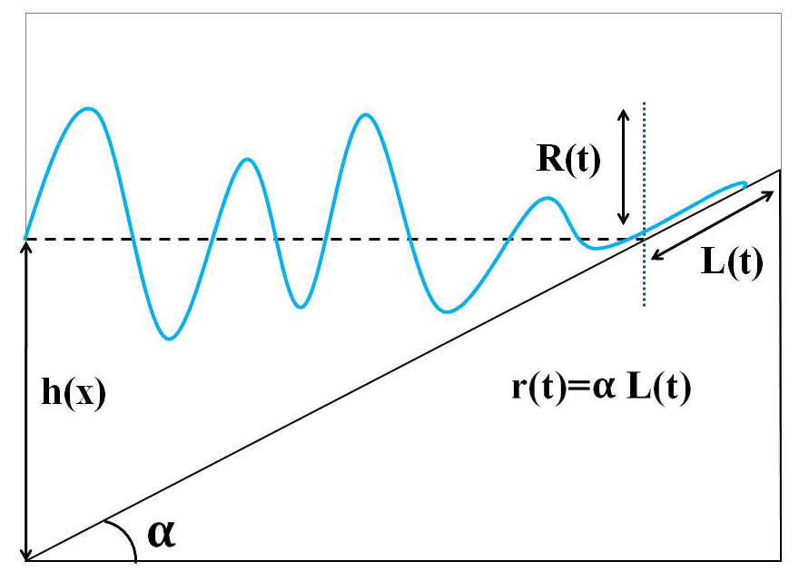
2 Basic equations and transformations

Here we will consider the classical formulation of the problem of a long-wave run-up on the constant-gradient slope in an ideal fluid (Fig. 1). The wave is one-dimensional and propagates along the x axis directed onshore. The basin depth is a linear depth function: $h (x) = - α x$ , where α is the inclination angle tangent and point x=0 corresponds to a fixed unperturbed water shoreline. L(t) and r(t) describe the horizontal and vertical displacement of the moving shoreline, and R(t) is the water level oscillations at x=0. The bottom and the shore are assumed to be impenetrable. The long-wave dynamics are described by nonlinear shallow-water equations:

\begin{array}{l} (1) & \frac{\partial u}{\partial t} + u \frac{\partial u}{\partial x} + g \frac{\partial η}{\partial x} = 0, \\ (2) & \frac{\partial η}{\partial t} + \frac{\partial}{\partial x} [(- α x + η) u] = 0 . \end{array}

Here, η(x, t) is the free surface elevation above the undisturbed water level, u(x, t) is the depth-averaged flow velocity (within the shallow-water theory, the flow velocity is the same on all horizons), and g is the gravity acceleration. Obviously, after introducing the total depth

\begin{matrix} (3) & H (x, t) = - α x + η (x, t), \end{matrix}

Eqs. (1) and (2) are a hyperbolic system with constant coefficients. This fact makes it possible to transform the system into a linear equation one by using a hodograph (Legendre) transformation, which was done in the pioneering work of Carrier and Greenspan in 1958. As a result, the wave field is described by a linear wave equation in the “cylindrical” coordinate system

\begin{matrix} (4) & \frac{\partial^{2} Φ}{\partial λ^{2}} - \frac{\partial^{2} Φ}{\partial σ^{2}} - \frac{1}{σ} \frac{\partial Φ}{\partial σ} = 0, \end{matrix}

and all variables are expressed in terms of an auxiliary wave function Φ(σ, λ) using explicit formulas

\begin{array}{l} (5) & η = \frac{1}{2 g} (\frac{\partial Φ}{\partial λ} - u^{2}), \\ (6) & u = \frac{1}{σ} \frac{\partial Φ}{\partial σ}, \\ (7) & x = \frac{1}{2 α g} (\frac{\partial Φ}{\partial λ} - u^{2} - \frac{σ^{2}}{2}), \\ (8) & t = \frac{1}{α g} (λ - u) . \end{array}

It should be noted that the variable σ is proportional to the total water depth.

\begin{matrix} (9) & σ = 2 \sqrt{g H} = 2 \sqrt{g (- α x + η)} \end{matrix}

Therefore, the wave equation (Eq. 4) is solved on the semiaxis σ≥0, and this coordinate plays the radius role in the cylindrical coordinate system. We would like to emphasize that the point σ=0 corresponds to a moving shoreline, and therefore the original problem, solved in the area with an unknown boundary, is reduced to the fixed area problem.

https://www.nat-hazards-earth-syst-sci.net/19/1925/2019/nhess-19-1925-2019-f01

Figure 1The problem geometry.

Download

It is important to note that the hodograph transformation is valid if the Jacobian transformation is nonzero

\begin{matrix} (10) & J = \frac{\partial (x, t)}{\partial (σ, λ)} \neq 0 . \end{matrix}

It is the case when a gradient catastrophe, identified in the framework of the shallow-water theory with the wave-breaking, does not occur. The necessary condition for the absence of wave-breaking is the boundedness and smoothness of all solutions; this question will be discussed below.

We will assume that the wave approaches the coast from the area far from the shoreline ( $x \to - \infty$ ), where the wave is linear. Then it is obvious that the function Φ(σ, λ) can be completely found from the linear theory. The difficulty in finding the wave field in the near-shoreline area is due to the implicit transformation of the coordinates (x, t) to (σ, λ). However, for the most interesting point of the moving shoreline σ=0 (its dynamics determines the size of the flooded area on the coast) all the formulas become explicit. In particular, from Eqs. (5) and (6) follows

\begin{array}{l} (11) & r (t) = R [t + \frac{u (t)}{α g}] - \frac{u (t)^{2}}{2 g}, \\ (12) & u (t) = U [t + \frac{u (t)}{α g}], \end{array}

where r(t) and u(t) are the vertical displacement of the moving shoreline and its speed, and the functions R(t) and U(t) determine the field characteristics at the fixed point (x=0) from the linear theory

\begin{matrix} (13) & \begin{aligned} R (t) = \frac{1}{2 g} {\frac{\partial Φ (σ = 0, λ)}{\partial λ}|}_{λ = α g t}, \\ U (t) = {\frac{1}{σ} \frac{\partial Φ (σ, λ)}{\partial σ}|}_{σ = 0, λ = α g t} . \end{aligned} \end{matrix}

Then we add the obvious kinematic relations for the vertical displacement and velocity of the last sea point along the slope

\begin{matrix} (14) & u (t) = \frac{1}{α} \frac{d r (t)}{d t}, U (t) = \frac{1}{α} \frac{d R (t)}{d t} . \end{matrix}

Let us note that Eq. (12) is identical to the so-called Riemann wave or a simple wave in a nonlinear, nondispersive medium (in particular, in nonlinear acoustics) if we consider the parameter 1∕αg to be a “coordinate”; see, for example, Rudenko and Soluyan (1977) and Gurbatov et al. (1991, 2011). Moreover, Eq. (11) describes the integral over the Riemann wave. This analogy proves to be very useful when transferring the already known results in the wave nonlinear theory to the run-up characteristics described by Eqs. (11) and (12).

Detailed calculations of the long-wave run-up on the coast were carried out repeatedly; see, for example, Carrier and Greenspan (1958), Synolakis (1987), Pelinovsky and Mazova (1992), Tinti and Tonini (2005), Madsen and Fuhrman (2008), Madsen and Schaffer (2010), Antuano and Brocchini (2008, 2010), Didenkulova (2009), Dobrokhotov et al. (2015), and Aydin and Kanoglu (2017).

It is worth mentioning that the nonlinear time transformation in Eqs. (11) and (12) leads to the shoreline oscillation distortion in comparison with the linear theory predictions. So, for large amplitudes the wave shape becomes multivalued (broken). The first moment of the wave breaking on the shoreline (the gradient catastrophe) is easily found from Eq. (12) by calculating the first derivative of the moving shoreline velocity

\begin{matrix} (15) & \frac{d u}{d t} = \frac{d U / dt}{1 - \frac{d U / d t}{α g}}, \end{matrix}

and from this follows the wave-breaking condition

\begin{matrix} (16) & Br = \frac{\max (d U / d t)}{α g} = \frac{\max (d^{2} R / d t^{2})}{α^{2} g} = 1, \end{matrix}

where we have introduced the breaking parameter Br to designate the left-hand side in Eq. (16), which characterizes the nonlinear wave properties on the shoreline. The condition (Eq. 16) can be given a physical meaning: that the breaking occurs when the last sea particle acceleration ( $α^{- 1} d^{2} R / d t^{2}$ ) exceeds the component of the gravity acceleration along the shoreline (gα). As shown in Didenkulova (2009), the condition (Eq. 16) coincides with Eq. (10) for Jacobian. It is important to emphasize that the breaking condition is unequivocally found through solving the linear problem of the wave run-up on the shore. It is determined only by the particle acceleration value on the shoreline, but it is not determined separately by the shoreline displacement or its velocity.

The similar Carrier–Greenspan transformation is obtained for waves in narrow-inclined channels, fjords, and bays (Rybkin et al., 2014; Pedersen, 2016; Anderson et al., 2017; Raz et al., 2018); only the wave equation (Eq. 4) and relations (Eqs. 5–8) change. However, the moving shoreline dynamics are still described by Eqs. (11) and (12), valid for arbitrary cross section channels.

3 The moving shoreline dynamics at an initially monochromatic wave run-up

The monochromatic wave run-up on a flat slope by using the Carrier–Greenspan transformation has been studied in a number of papers cited above. Let us reproduce here the main features of the moving shoreline dynamics necessary for us to draw the statistical description below. Mathematically, the monochromatic wave run-up is described by an elementary solution of Eq. (4)

\begin{matrix} (17) & Φ (σ, λ) = Q J_{0} (l σ) \cos (l λ), \end{matrix}

where Q and l are arbitrary constants and J₀ is the zero-order Bessel function. Far from the shoreline (σ→∞) the Bessel function decreases, so the wave function Φ becomes small. In this case, in Eqs. (5)–(8) one can use approximate expressions (the “linear” Carrier–Greenspan transformation)

\begin{matrix} (18) & η = \frac{1}{2 g} \frac{\partial Φ}{\partial λ}, u = \frac{1}{σ} \frac{\partial Φ}{\partial σ}, x = - \frac{σ^{2}}{4 α g}, t = \frac{λ}{α g}, \end{matrix}

and, using the asymptotic representation for the Bessel function, reduce Eq. (17) to the expression for the water surface displacement

\begin{matrix} (19) & \begin{aligned} η (x, t) & = a (x) \{\sin [ω (t - \int \frac{d x}{\sqrt{g h (x)}})] - \frac{π}{4}\} \\ + \sin [ω (t + \int \frac{d x}{\sqrt{g h (x)}}) + \frac{π}{4}], \end{aligned} \end{matrix}

where

\begin{matrix} (20) & a (x) = \frac{Q}{2 g} \sqrt{\frac{l}{π \sqrt{g h (x)}}}, ω = g l α . \end{matrix}

The wave field away from the shoreline is a superposition of two waves of the same frequency and a variable amplitude a(x), which together form a standing wave. It immediately shows that the wave amplitude varies with depth according to Green's law ( $h^{- 1 / 4}$ ), as it should be far from the coast. The same asymptotic result follows from the exact solution of linear shallow-water equations

\begin{matrix} (21) & η (x, t) = R_{0} J_{0} (\sqrt{\frac{4 ω^{2} | x |}{g α}}) \sin (ω t), \end{matrix}

where R₀ is the wave amplitude at the fixed shoreline (x=0), identified with the maximum run-up height in the linear theory. By connecting Eqs. (20) and (21), we obtain the formula for the run-up height obtained through the incident wave amplitude far from the coast

\begin{matrix} (22) & \frac{R_{0}}{a (x)} = \sqrt{\frac{2 ω}{α} \sqrt{\frac{h (x)}{g}}} . \end{matrix}

Equation (22) allows for working further with the run-up height R₀ instead of the wave amplitude far from the coast a(x). This run-up height will be considered the given value. Having determined Q and l through the incident wave parameters, we can calculate the run-up characteristics in the nonlinear theory, considering the limit of Eq. (17) with σ→0 and using the Carrier–Greenspan transformation formulas (Eqs. 5–8). The moving shoreline movement is determined by the parametric dependence

\begin{array}{l} (23) & t = \frac{λ}{α g} - \frac{ω R_{0}}{α^{2} g} \cos (\frac{ω λ}{α g}), \\ (24) & r = R_{0} \sin (\frac{ω λ}{α g}) - \frac{ω^{2} R_{0}^{2}}{2 α^{2} g} \cos^{2} (\frac{ω λ}{α g}) . \end{array}

It is convenient to introduce dimensionless variables

\begin{matrix} (25) & z = \frac{r}{R_{0}}, τ = ω t, φ = \frac{ω λ}{α g}, \end{matrix}

and calculate the breaking parameter

\begin{matrix} (26) & Br = \frac{ω^{2} R_{0}}{α^{2} g}, \end{matrix}

so Eqs. 23 and 24 are finally rewritten in the form

\begin{array}{l} (27) & τ = φ - Br \cos (φ), \\ (28) & z = \sin (φ) - \frac{Br}{2} \cos^{2} (φ), \end{array}

which is another expression for Eqs. (11) and (12) if we take

\begin{matrix} (29) & R (t) = R_{0} \sin (ω t), \end{matrix}

arising from Eq. (21) with x=0. Let us note that the function z(τ, Br) is set in a parametric form, but after expressing φ from Eq. (28) and substituting it in Eq. (27), we can obtain the explicit expression for the function τ(z; Br). In this paper, we will use both explicit and implicit expressions of the functions describing the moving shoreline dynamics.

Figure 2 shows the moving shoreline dynamics at different wave height values in terms of the breaking parameter up to the limiting value (Br = 1). In the limit of small parameter values, the oscillations are close to sinusoidal (it is almost a linear problem). Then, with the increasing amplitude, the moving shoreline velocity gets a steep leading front, while at the moving shoreline vertical displacement a peculiar feature is formed at the wave run-down stage. As it is known, at the time of the Riemann wave breaking, the peculiarity like $u \sim t^{1 / 3}$ is formed (Pelinovsky et al., 2013). Then, in the integral over the Riemann wave (at the moving shoreline displacement), this peculiar feature will have the form $z \sim t^{4 / 3}$ . Thus, with the wave amplitude increase, the first breaking occurs at sea (at the run-down stage) and not on the coast. Then the breaking zone expands and moves on to the sea, but at this stage, analytical solutions based on the Carrier–Greenspan transformation become inapplicable.

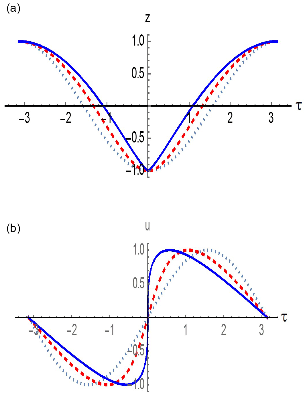
https://www.nat-hazards-earth-syst-sci.net/19/1925/2019/nhess-19-1925-2019-f02

Figure 2The moving shoreline dynamics (a) and its velocity (b) in the case of the incident monochromatic wave for different breaking parameter values Br (0: the dotted line; 0.5: the dashed line; 1: the solid line).

Download

4 Probabilistic characteristics of the initially sine wave run-up with a random phase

Let us now consider the probabilistic characteristics of the initially sine wave run-up with a random phase on the shore, assuming it to be uniformly distributed over the interval [0–2π]. These characteristics are found by using the geometric probability methods (Kendall and Stuart, 1969), so that for ergodic processes the probability density of the moving shoreline vertical displacement coincides with the relative location time of the function z(τ) in the interval (z, z+dz)

\begin{matrix} (30) & W (z) = \frac{1}{2 π} \sum_{n = 1}^{N} |\frac{d τ_{n}}{d z}|, \end{matrix}

where the summation takes place at all intersection levels z(τ). For harmonic disturbance, it is enough to restrict ourselves to considering the field over a half-period. So, for the moving shoreline vertical displacement in dimensionless variables, the derivative dτ∕dz of the parametric curve (Eqs. 27 and 28) can be calculated through the ratio of the derivatives dτ∕dφ and dz∕dφ

\begin{matrix} (31) & W_{z}^{\sin} (z; Br) = \frac{1}{π} \frac{1 + Br \sin φ}{\cos φ + Br \cos φ \sin φ} = \frac{1}{π \cos φ} . \end{matrix}

We indicated here that the probability density depends on Br as a parameter. Finding cos φ from Eq. (28) for the vertical displacement, we obtain the final expression for the probability density

\begin{matrix} (32) & W_{z}^{\sin} (z; Br) = \frac{1}{π} \frac{1}{\sqrt{1 - \frac{1}{{Br}^{2}} {[1 - \sqrt{1 + 2 z Br + {Br}^{2}}]}^{2}}}, \end{matrix}

which in the linear problem for a purely sinusoidal perturbation transforms into a well-known expression for the probability distribution of a harmonic signal with a random phase (Kendall and Stuart, 1969)

\begin{matrix} (33) & W_{z}^{\sin} (z; 0) = \frac{1}{π} \frac{1}{\sqrt{1 - z^{2}}} . \end{matrix}

The probability distribution (Eq. 32) for the three values of the parameter Br is shown in Fig. 3. As you can see, the probability density becomes an asymmetric function with a greater probability in the area of positive values corresponding to the wave run-up on the coast than at the run-down stage. At the ends of the interval, the probability density is unlimited throughout the entire range change of Br, since the shoreline oscillations near the maximum have a zero derivative (the moving shoreline velocity in it becomes zero).

https://www.nat-hazards-earth-syst-sci.net/19/1925/2019/nhess-19-1925-2019-f03

Figure 3The probability density of the moving shoreline vertical displacement for the initially sine wave run-up at Br = 0 (the dotted line), 0.5 (the dashed line), and 1 (the solid line).

Download

The obtained probability density function can be used to calculate the statistical moments of the shoreline oscillations. Technically, however, it is easier to use the parametric equations (Eqs. 27 and 28) and calculate all the moments.

\begin{matrix} (34) & M_{n}^{z} = \frac{1}{2 π} \int_{0}^{2 π} z^{n} (τ) d τ = \frac{1}{2 π} \int_{0}^{2 π} z^{n} (φ) \frac{d τ}{d φ} d φ \end{matrix}

Thus, the first moment,

\begin{matrix} (35) & M_{1}^{z} = \frac{Br}{4}, \end{matrix}

determines the average water level rise on the coast when the waves approach the shore (the setup phenomenon), which is commonly observed (Dean and Walton, 2009).

The second moment determines the dispersion

\begin{matrix} (36) & δ^{2} = \frac{1}{2 π} \int_{0}^{2 π} {(z - M_{1}^{z})}^{2} d τ = \frac{1}{2} - \frac{3}{32} {Br}^{2}, \end{matrix}

characterizing the fluctuation range relative to the average value; it relatively weakly decreases with the growth of the parameter Br (less than 10 % for non-breaking waves).

Finally, the total flooding time and its drainage time are easy to find from Eqs. (27) and (28) by finding from the Eq. (28) the value φ at which z=0 and substituting the obtained values in Eq. (27)

\begin{matrix} (37) & \begin{aligned} T_{flood} & = π - 2 \arcsin [\frac{\sqrt{1 + {Br}^{2}} - 1}{Br}] \\ + 2 \sqrt{2} \sqrt{\sqrt{1 + {Br}^{2}} - 1}, \end{aligned} \\ (38) & \begin{aligned} T_{dry} & = π + 2 \arcsin [\frac{\sqrt{1 + {Br}^{2}} - 1}{Br}] \\ - 2 \sqrt{2} \sqrt{\sqrt{1 + {Br}^{2}} - 1} . \end{aligned} \end{matrix}

Both times change almost linearly with the increasing wave amplitude (parameter Br); see Fig. 4.

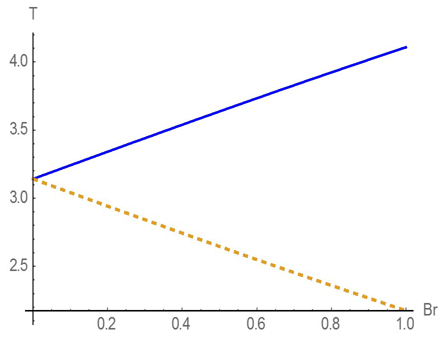
https://www.nat-hazards-earth-syst-sci.net/19/1925/2019/nhess-19-1925-2019-f04

Figure 4The total flooding time (the solid curve) and the drainage time (the dashed curve) depending on the parameter Br.

Download

It is worth noting that, in contrast to the vertical displacement, the moving shoreline velocity distribution [ $u = (ω R_{0} / α) v$ ], as it is easy to show, does not depend on the breaking parameter, and the probability density function is determined by the simple formula

\begin{matrix} (39) & W_{v}^{\sin} (v) = \frac{1}{π} \frac{1}{\sqrt{1 - v^{2}}} . \end{matrix}

The distribution independence on the degree of nonlinearity is well known for the Riemann waves and is explained by the compensation of compression and rare fraction areas (Gurbatov et al., 1991, 2011).

5 Probabilistic characteristics of a narrow-band wave run-up with a random amplitude and phase

Let us consider the run-up of a quasi-harmonic wave with a random amplitude and phase on a flat slope. To do this, we will first rewrite Eqs. (32) and (37) for them to include the wave amplitude. It is convenient to enter the maximum height R_max as the amplitude scales at which the breaking parameter turns into 1

\begin{matrix} (40) & Br = \frac{ω^{2} R_{\max}}{α^{2} g} = 1, \end{matrix}

and to use the dimensionless displacement ( $y = r / R_{\max}$ ). Then the dimensionless amplitude is

\begin{matrix} (41) & A = \frac{R_{0}}{R_{\max}} \leq 1, \end{matrix}

and Eq. (32) is converted to the form ( $- A < y < A$ )

\begin{matrix} (42) & W_{y}^{\sin} (y; A) = \frac{1}{π} \frac{1}{\sqrt{A^{2} - {[1 - \sqrt{1 + 2 y + A^{2}}]}^{2}}} . \end{matrix}

Assuming now that the wave amplitude A is a random variable, we average Eq. (40) by using the amplitude distribution density W_A(A)

\begin{matrix} (43) & W (y) = \int_{y}^{\infty} W_{y}^{\sin} (y; A) W_{A} (A) d A . \end{matrix}

Equation (43) has an important practical meaning: by using the measured distribution of the wave amplitudes far from the coast (recomputed on run-up amplitudes in the linear theory), it is possible to obtain the distribution of the wave run-up characteristics on the coast. The only requirement imposed on the wave ensemble is that it should not contain breaking waves, which should be somehow removed from the record. It immediately follows that the Gaussian field containing large amplitude tails does not fit this requirement, and it should be modified. Therefore, we assume the amplitude distribution to be finite for $A < A_{\max} = 1$ . The narrow-band random wave field contains sine waves with almost constant frequency and random amplitude and phase. It means that if the wave amplitude is below the “breaking amplitude” A_max=1, the breaking will not be implemented in any way, and the random wave run-up will take place without any breaking. Further calculations depend on the specific type of the amplitude distribution.

Let us construct the finite amplitude distribution at which the linear field distribution is close to the Gaussian form and modify the Rayleigh distribution for wave heights in the area $A < A_{\max} = 1$ (Fig. 5)

\begin{matrix} (44) & \begin{aligned} W_{A} (A; A_{\max}, A_{s}) = & \frac{1}{1 - \exp (- 2 A_{\max}^{2} / A_{s}^{2})} \frac{4 A}{A_{s}^{2}} \\ \exp (- 2 \frac{A^{2}}{A_{s}^{2}}), A \leq A_{\max}, \end{aligned} \end{matrix}

to make the density function distribution normalized. Here, A_s is the so-called significant wave run-up height (an averaged value of one-third of the highest amplitudes). We would like to note here that it follows from Eqs. (11) and (12) that the extremal run-up characteristics in the nonlinear theory remain the same as in the linear theory. This means that the significant wave run-up height remains the same as in the nonlinear theory.

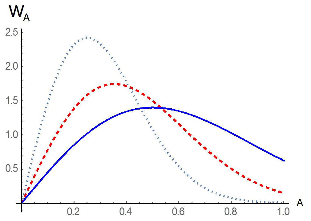
https://www.nat-hazards-earth-syst-sci.net/19/1925/2019/nhess-19-1925-2019-f05

Figure 5The modified Rayleigh distribution (Eq. 43) for different distribution values A_s∕A_max (0.5: the dotted curve; 0.7: the dashed line; 1: the solid line).

Download

When $A_{s} ≪ A_{\max} = 1$ , the distribution (Eq. 44) transforms into the Rayleigh one, which is characteristic of the Gaussian initial distribution of a narrow-band random signal. With the help of Eq. (43), it becomes possible to calculate the distribution function of shoreline oscillations for the various wave energies. So, with the incident wave small amplitude (A_s≪1), the distribution (Eq. 44) can be replaced by a simpler expression (Eq. 33) and the answer is the run-up distribution characteristics in the linear theory:

\begin{matrix} (45) & \begin{aligned} W_{lin} & (y; A_{\max}, A_{s}) = \frac{4}{π A_{s}^{2} [1 - \exp (- 2 A_{\max}^{2} / A_{s}^{2})]} \\ \int_{y}^{A_{\max}} \frac{A}{\sqrt{A^{2} - y^{2}}} \exp (- 2 \frac{A^{2}}{A_{s}^{2}}) d A . \end{aligned} \end{matrix}

Besides, if $A_{s} ≪ A_{\max} = 1$ , the integral (Eq. 45) is reduced to the Gaussian distribution

\begin{matrix} (46) & W_{lin} (y; A_{s}) = \frac{2}{\sqrt{2 π} A_{s}} \exp (- 2 \frac{y^{2}}{A_{s}^{2}}), \end{matrix}

where A_s=2σ_y and $σ_{y}^{2}$ is the moving shoreline oscillation dispersion.

Figure 6 shows the distribution of the run-up characteristics for different ratios of A_s∕A_max values by Eqs. (43) and (44); they are shown in solid lines. Here the dashed lines show the calculation results according to the linear theory (Eq. 46). As one can see, with $A_{s} / A_{\max} = 0.5$ (Fig. 6a) and 0.7 (Fig. 6b), the linear distribution is close to the Gaussian one. Nonlinearity leads to the asymmetry of the distribution function density in the direction of positive values corresponding to the wave characteristics on the coast. If the undisturbed wave ensemble is made of relatively large waves ( $A_{s} / A_{\max} = 1$ ), their distribution is far from the Gaussian, both in the linear and in the nonlinear approximation.

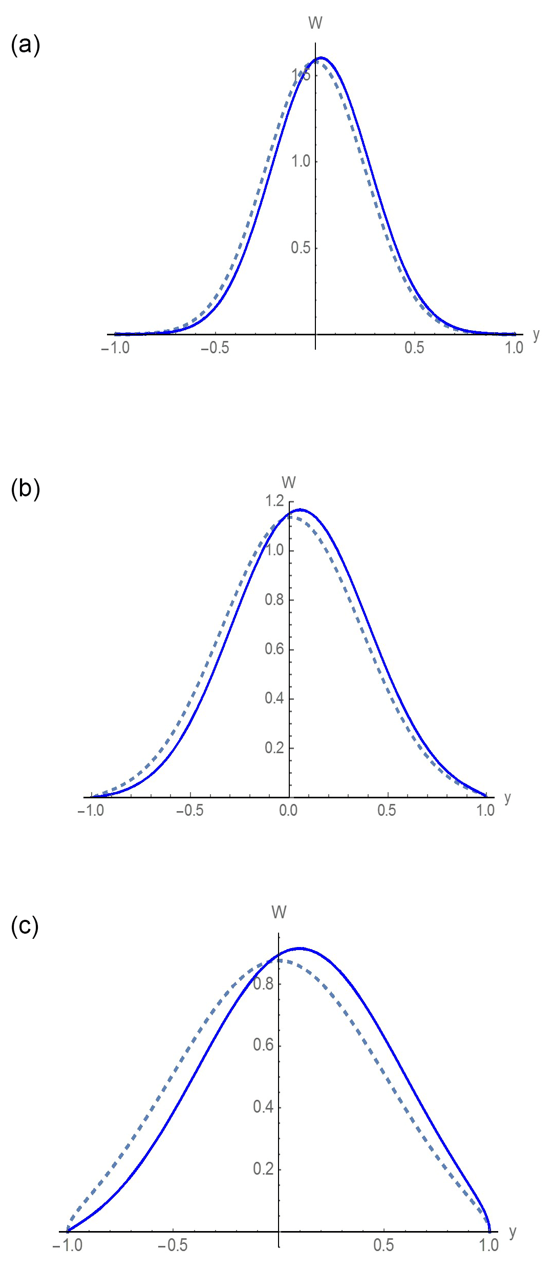
https://www.nat-hazards-earth-syst-sci.net/19/1925/2019/nhess-19-1925-2019-f06

Figure 6The probabilistic density function of the vertical shoreline displacement in the nonlinear theory (the solid lines) and in the linear theory (the dashed lines) for different A_s∕A_max: (a) 0.5 values, (b) 0.7, and (c) 1 .

Download

The finite (A<A_max) power-law distribution concentrated mainly near the maximum amplitude A_max can be considered to be another example of undisturbed large-amplitude waves.

\begin{matrix} (47) & W_{A} (A) = \frac{6 A^{5}}{A_{\max}^{6}} \end{matrix}

Figure 7 shows the graphs of the probabilistic density function of the moving shoreline displacement calculated by using Eq. (46) in the linear theory and Eq. (43) in the nonlinear theory. It is also seen in the figure that the nonlinear effects lead to a strong asymmetry towards the positive values, i.e., to the wave amplification at the run-up stage than at the run-down stage.

https://www.nat-hazards-earth-syst-sci.net/19/1925/2019/nhess-19-1925-2019-f07

Figure 7The probabilistic density function of the shoreline vertical displacement in the linear theory (the dashed line) and nonlinear theory (the solid line).

Download

6 The wave-breaking effect on probabilistic run-up characteristics

The theory described above is valid for non-breaking waves. The mentioned wave ensemble, strictly speaking, cannot be the Gaussian one, as it always has unlimited tails in the probability density function. Let us briefly discuss what the formulas obtained for non-breaking waves lead to in the presence of broken waves. Figure 8 shows the parametric curve (Eqs. 27 and 28) when Br = 2. Formally, the curve became multivalued in the range of negative values corresponding to the maximum water outflow from the coast. We have already indicated that the probability density function of the moving shoreline vertical displacement W(ξ) coincides with the relative residence time ξ(t) of the function in the interval (ξ, ξ+dξ), which is calculated by Eq. (17). In contrast to negative cut-off bias values, in the area of positive values there is no ambiguity, and therefore all the calculations can be carried out by using the formulas described above. The calculation example with Br = 2 and $r > - 0.5$ (in the zone of one-value solution) is shown in Fig. 9. However, these results should be treated with caution. If Br > 1 the Jacobian breaks down seawards of the shoreline. This may affect the probabilistic distribution on the positive side. This important issue requires going beyond the theory discussed in this article.

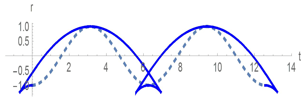
https://www.nat-hazards-earth-syst-sci.net/19/1925/2019/nhess-19-1925-2019-f08

Figure 8The parametric curve (Eqs. 27 and 28) with Br = 2 (the solid curve) in comparison with the linear problem with Br = 0 (the dashed line).

Download

https://www.nat-hazards-earth-syst-sci.net/19/1925/2019/nhess-19-1925-2019-f09

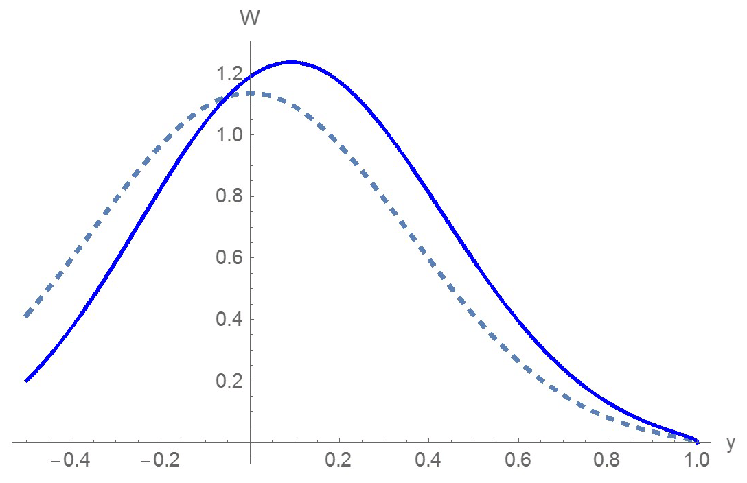
Figure 9The probability density function at Br = 2, constructed by Eqs. (42) and (43) (the solid line) in comparison with the linear distribution (Eq. 43) (the dotted line) ( $A_{s} / A_{\max} = 0.7$ ).

Download

7 Discussion and conclusion

In this paper, we study the run-up of irregular narrow-band waves with a random envelope (swell, storm surges, and tsunami) on a beach of a constant slope. The work was carried out in the framework of the nonlinear wave theory with one important assumption: there should be no breaking waves in the wave ensemble. This restriction is quite strict for field and laboratory conditions, but nevertheless, there are cases when it is performed. For instance, 75 % of historical tsunami waves climbed onto the coast with no breaking (Mazova et al., 1983). In the experiments performed in the Warwick University tank and in the Large Tank in Hanover (Denissenko et al., 2011, 2013) this condition was fulfilled.

The wave nonlinearity at the run-up stage leads to increased deviations from Gaussianity, as might be expected from general considerations. Nevertheless, it is shown that the probability distribution of the moving shoreline velocity does not depend on the wave nonlinearity and can be calculated within the linear theory framework. The same conclusion can be drawn about the distribution of the extreme run-up characteristics (the moving shoreline displacement and speed), which, in fact, has been discussed previously (Didenkulova et al., 2008). However, the probabilistic density function of the moving shoreline displacement differs from that predicted in the linear theory framework. It is described by Eq. (43) by using either the theoretical or the measured distribution of the incident wave amplitudes. The paper gives the calculation results of the probabilistic run-up characteristics with the modified Rayleigh distribution for wave amplitudes.

The wave-breaking leads to the inapplicability of the wave run-up theory based on the Carrier–Greenspan transformation. If, nevertheless, the share of large amplitude waves is small, the breaking occurs mainly at the run-down stage, having little effect on the long-wave coastal flooding characteristics (see Sect. 6). This question, however, requires a special study based on direct numerical solutions of the shallow-water equations or their nonlinear-dispersive generalizations.

Finally, it is worth noting that we considered the narrow-band wave run-up with a random amplitude and phase. As far as the random waves with a wide spectrum are concerned, they may be the problem for further consideration.

The obtained probability density functions of the vertical displacement of the moving shoreline are useful to compute statistical characteristics of flooding time and force on coasts and constructions, which are necessity for the mitigation of natural marine hazards.

Now, in practice, various generalizations of shallow-water equations are used to analyze tsunami run-up including the wave dispersion; see, for instance, Løvholt et al. (2012). The wave dissipation is a quadratic dissipative term that prevents us from getting analytical results, so its influence on statistical characteristics should be investigated in the future.

Data availability

All data have been obtained using the analytic formulas given in the text.

Author contributions

SG performed the computing of the random Riemann wave characteristics, and EP performed the computations of the probability density function of the moving shoreline.

Competing interests

The authors declare that they have no conflict of interest.

Acknowledgements

The work is supported by the grants from the Russian Science Foundation: grant nos. 19-12-00256 (for computing the random Riemann wave characteristics) and 16-17-00041 (for the computations of the probability density function of the moving shoreline).

Financial support

This research has been supported by the Russian Science Foundation (grant nos. 19-12-00256 and 16-17-00041).

Review statement

This paper was edited by Ira Didenkulova and reviewed by two anonymous referees.

References

Anderson, D., Harris, M., Hartle, H., Nicolsky, D., Pelinovsky, E., Raz, A., and Rybkin, A.: Runup of long waves in piecewise sloping U-shaped bays, Pure Appl. Geophys., 174, 3185–3207, 2017.

Antuano, M. and Brocchini, M.: Maximum run-up, breaking conditions and dynamical forces in the swash zone: a boundary value approach, Coast. Eng., 55, 732–740, 2008.

Antuano, M. and Brocchini, M.: Solving the nonlinear shallow-water equations in physical space, J. Fluid Mech., 643, 207–232, 2010.

Aydin, B. and Kanoglu, U.: New analytical solution for nonlinear shallow water-wave equations, Pure Appl. Geophys., 174, 3209–3218, 2017.

Bec, J. and Khanin, K.: Burgers turbulence, Phys. Rep., 447, 1–66, 2007.

Burgers, J. M.: The Nonlinear Diffusion Equation, D. Reidel, Dordrecht, 1974.

Carrier, G. F.: On-shelf tsunami generation and coastal propagation, in: Tsunami: Progress in Prediction, Disaster Prevention and Warning, edited by: Tsuchiya, Y. and Shuto, N., Kluwer, Dordrecht, 1–20, 1995.

Carrier, G. F. and Greenspan, H. P.: Water waves of finite amplitude on a sloping beach, J. Fluid Mech., 4, 97–109, 1958.

Carrier, G. F., Wu, T. T., and Yeh, H.: Tsunami run-up and draw-down on a plane beach, J. Fluid Mech., 475, 79–99, 2003.

Choi, J., Kwon, K. K., and Yoon, S. B.: Tsunami inundation simulation of a built-up area using equivalent resistance coefficient, Coast. Eng. J., 54, 1250015, https://doi.org/10.1142/S0578563412500155, 2012.

Dean, R. G. and Walton, T. L.: Wave setup, in: Handbook of Coastal and Ocean Engineering, edited by: Kim, Y. C., World Sci, Singapore, 2009.

Denissenko, P., Didenkulova, I., Pelinovsky, E., and Pearson, J.: Influence of the nonlinearity on statistical characteristics of long wave runup, Nonlin. Processes Geophys., 18, 967–975, https://doi.org/10.5194/npg-18-967-2011, 2011.

Denissenko, P., Didenkulova, I., Rodin, A., Listak, M., and Pelinovsky E.: Experimental statistics of long wave runup on a plane beach, J. Coast. Res., 65, 195–200, 2013.

Didenkulova, I. I.: New trends in the analytical theory of long sea wave runup, in: Applied Wave Mathematics: Selected Topics in Solids, Fluids, and Mathematical Methods, edited by: Quak, E. and Soomere, T., Springer, Berlin, Heidelberg, 265–296, 2009.

Didenkulova, I. I., Pelinovsky, E., and Sergeeva, A.: Runup of long irregular waves on plane beach, in: Extreme Ocean Waves, edited by: Pelinovsky, E. and Kharif, C., Springer, Heidelberg, New York, Dordrecht, London, 83–94, 2008.

Didenkulova, I. I., Sergeeva, A. V., Pelinovsky, E. N., and Gurbatov, S. N.: Statistical estimates of characteristics of long wave run up on the shore, Izvestiya, Atmos. Ocean. Phys., 46, 530–532, 2010.

Didenkulova, I. I., Pelinovsky, E., and Sergeeva, A.: Statistical characteristics of long waves nearshore, Coast. Eng., 58, 94–102, 2011.

Dobrokhotov, S. Y., Minenkov, D. S., Nazaikinskii, V. E., and Tirozzi, B.: Simple exact and asymptotic solutions of the 1D run-up problem over a slowly varying (quasiplanar) bottom, in: Theory and Applications in Mathematical Physics, World Scientific, Singapore, 29–47, 2015.

Frisch, U.: Turbulence: the legacy of A. N. Kolmogorov, Cambridge University Press, Cambridge, 1995.

Frisch, U. and Bec, J.: Burgulence, in: New trends in turbulence, edited by: Lesieur, M., Yaglom, A., and David, F., Springer-Verlag, Berlin, Heidelberg, 341–383, 2001.

Gurbatov, S. N. and Saichev, A. I.: Inertial nonlinearity and chaotic motion of particle fluxes, Chaos, 3, 333–358, 1993.

Gurbatov, S. N., Malakhov, A. N., and Saichev, A. I.: Nonlinear Random Waves and Turbulence in Nondispersive Media: Waves, Rays, Particles, Manchester University Press, Manchester, 1991.

Gurbatov, S. N., Simdyankin, S., Aurell, E., Frisch, U., and Toth, G.: On the decay of Burgers turbulence, J. Fluid Mech., 344, 349–374, 1997.

Gurbatov, S. N., Rudenko, O. V., and Saichev, A. I.: Waves and Structures in Nonlinear Nondispersive Media, Springer-Verlag, Berlin, Heidelberg and Higher Education Press, Beijing, 2011.

Gurbatov, S. N., Saichev, A. I. and Shandarin, S. F.: Large-scale structure of the Universe. The Zeldovich approximation and the adhesion model, Physics Uspekhi, 55, 223–249, 2012.

Gurbatov, S. N., Deryabin, M. S., Kasyanov, D. A., and Kurin, V. V.: Evolution of narrow-band noise beams for large acoustic Reynolds numbers, Radiophys. Quant. Elect., 61, 478–490, 2018.

Gurbatov, S. N., Deryabin, M., Kurin, V., and Kasyanov, D.: Evolution of intense narrowband noise beams, J. Sound Vibrat., 439, 208–218, 2019.

Harris, M. W., Nicolsky, D. J., Pelinovsky, E. N., and Rybkin, A. V.: Runup of nonlinear long waves in trapezoidal bays: 1-D analytical theory and 2-D numerical computations, Pure Appl. Geophys., 172, 885–899, 2015.

Harris, M. W., Nicolsky, D. J., Pelinovsky, E. N., Pender, J. M. and Rybkin, A. V.: Run-up of nonlinear long waves in U-shaped bays of finite length: Analytical theory and numerical computations, J. Ocean Eng. Mar. Energy, 2, 113–127, 2016.

Hughes, M. G., Moseley, A. S., and Baldock, T. E.: Probability distributions for wave runup on beaches, Coast. Eng., 57, 575–584, 2010.

Huntley, D. A., Guza, R. T. and Bowen, A. J.: A universal form for shoreline run-up spectra, J. Geophys. Res., 82, 2577–2581, 1977.

Kaiser, G., Scheele, L., Kortenhaus, A., Løvholt, F., Römer, H., and Leschka, S.: The influence of land cover roughness on the results of high resolution tsunami inundation modeling, Nat. Hazards Earth Syst. Sci., 11, 2521–2540, https://doi.org/10.5194/nhess-11-2521-2011, 2011.

Kendall, M. G. and Stuart, A.: The Advanced Theory of Statistics, in: Volume I, Distribution Theory, Wiley, London, 1969.

Kian, R., Velioglu, D., Yalciner, A. C., and Zaytsev, A.: Effects of harbor shape on the induced sedimentation; L-type basin, J. Mar. Sci. Eng., 4, 55–65, 2016.

Løvholt, F., Pedersen, G., Bazin, S., Kühn, D., Bredesen, R. E., and Harbitz, C.: Stochastic analysis of tsunami runup due to heterogeneous coseismic slip and dispersion, J. Geophys. Res., 117, C03047, https://doi.org/10.1029/2011JC007616, 2012.

Macabuag, J., Rossetto, T., Ioannou, I., Suppasri, A., Sugawara, D., Adriano, B., Imamura, F., Eames, I., and Koshimura, S.: A proposed methodology for deriving tsunami fragility functions for buildings using optimum intensity measures, Nat. Hazards, 84, 1257–1285, 2016.

Madsen, P. A. and Fuhrman, D. R.: Run-up of tsunamis and long waves in terms of surf-similarity, Coast. Eng., 55, 209–223, 2008.

Madsen, P. A. and Schaffer, H. A.: Analytical solutions for tsunami runup on a plane beach: single waves, N-waves and transient waves, J. Fluid Mech., 645, 27–57, 2010.

Mazova, R. K., Pelinovsky, E. N., and Solov'yev, S. L.: Statistical data on the tsunami runup onto shore, Oceanology, 23, 698–702, 1983.

Molchanov, S. A., Surgailis, D., and Woyczynski, W. A.: Hyperbolic asymptotics in Burgers' turbulence and extremal processes, Comm. Math. Phys., 168, 209–226, 1995.

Ozer, S. C., Yalciner, A. C., and Zaytsev, A.: Investigation of tsunami hydrodynamic parameters in inundation zones with different structural layouts, Pure Appl. Geophys., 172, 931–952, 2015a.

Ozer, S. C., Yalciner, A. C., Zaytsev, A., Suppasri, A., and Imamura, F.: Investigation of hydrodynamic parameters and the effects of breakwaters during the 2011 Great East Japan Tsunami in Kamaishi Bay, Pure Appl. Geophys., 172, 3473–3491, 2015b.

Park, H., Cox, D. T., and Barbosa, A. R.: Comparison of inundation depth and momentum flux based fragilities for probabilistic tsunami damage assessment and uncertainty analysis, Coastal Eng., 122, 10–26, 2017.

Pelinovsky, D., Pelinovsky, E., Kartashova, E., Talipova, T., and Giniyatullin, A.: Universal power law for the energy spectrum of breaking Riemann waves, JETP Lett., 98, 237–241, 2013.

Pelinovsky, E. and Mazova, R.: Exact analytical solutions of nonlinear problems of tsunami wave run-up on slopes with different profiles, Nat. Hazards, 6, 227–249, 1992.

Pedersen, G.: Fully nonlinear Boussinesq equations for long wave propagation and run-up in sloping channels with parabolic cross sections, Nat. Hazards, 84, S599–S619, 2016.

Qi, Z. X., Eames, I., and Johnson, E. R.: Force acting on a square cylinder fixed in a free-surface channel flow, J. Fluid Mech., 756, 716–727, 2014.

Raz, A., Nicolsky, D., Rybkin, A., and Pelinovsky, E.: Long wave run-up in asymmetric bays and in fjords with two separate heads, J. Geophys. Res.-Oceanus, 123, 2066–2080, 2018.

Rudenko, O. V. and Soluyan, S. I.: Nonlinear Acoustics, Pergamon Press, New York, NY, 1977.

Rybkin, A. Pelinovsky, E. N., and Didenkulova, I.: Nonlinear wave run-up in bays of arbitrary cross-section: generalization of the Carrier-Greenspan approach, J. Fluid Mech., 748, 416–432, 2014.

Shimozono, T.: Long wave propagation and run-up in converging bays, J. Fluid Mech., 798, 457–484, 2016.

Synolakis, C. E.: The runup of solitary waves, J. Fluid Mech., 185, 523–545, 1987.

Synolakis, C. E., Bernard, E. N., Titov, V. V., Kanoglu, U., and Gonzalez, F. I.: Validation and verification of tsunami numerical models, Pure Appl. Geophys., 165, 2197–2228, 2008.

Tinti, S. and Tonini, R.: Analytical evolution of tsunamis induced by near-shore earthquakes on a constant-slope ocean, J. Fluid Mech., 535, 33–64, 2005.

Woyczynski, W. A.: Burgers – KPZ Turbulence, in: Gottingen Lectures, Springer-Verlag, Berlin, 1998.

Xiong, Y., Liang, Q., Park, H., Cox, D., and Wang, G.: A deterministic approach for assessing tsunami-induced building damage through quantification of hydrodynamic forces, Coast. Eng., 144, 1–14, 2019.