2.1 FwDET v2.0

FwDET calculates water depth by subtracting the calculated floodwater elevation (above mean sea level, a.m.s.l.) from topographic elevation at each grid cell within the flooded domain. The flooded domain is provided as a GIS polygon layer to FwDET, making the tool agnostic to the source and method used to derive the inundation extent. Elevation of each grid cell and the floodwater is derived from a digital elevation model (DEM). While any DEM can be used, its horizontal and vertical resolutions can have a major impact on the tool's accuracy. This is discussed in more detail below as well as in Cohen et al. (2018a, b). The core of the FwDET algorithm is the identification of local floodwater elevation. FwDET water depth calculation follows this following procedure (described and illustrated in detail in Cohen et al., 2018a): (1) conversion of the inundation polygon to a line layer, (2) creation of a raster layer from the line layer that has the same grid cell size and alignment as the DEM, (3) extraction of the DEM value (elevation) for these grid cells (referred to as boundary grid cells), (4) allocation of the local floodwater elevation for each grid cell within the flooded domain from its nearest boundary grid cell, and (5) floodwater depth calculation by subtracting local floodwater elevation from topographic elevation at each grid cell within the flooded domain.

For flooding within a river floodplain, associating the appropriate boundary grid cell is relatively straightforward as illustrated in Fig. 1 (top) with a cross section. In noncontinuous flood domains (e.g., in floodplains of braided rivers), isolated areas of non-flooded land can, and do quite often, exist. Non-flooded isolated areas can be real or represent an error in the remote sensing analysis due to, for example, undetected flooding under dense vegetation. FwDET identifies the cells around these areas as boundary grid cells, which, if these are real non-flooded (elevated) areas, is expected to improve the water depth calculations as it provides more localized floodwater elevation data. In coastal floods, the inundation polygon boundary at the coastline or ocean waters cannot be used as boundary grid cells since the DEM-extracted elevation will not represent the floodwater depth as illustrated in Fig. 1 (bottom). These boundary grid cells should, therefore, be excluded from the analysis. In FwDET v2.0 this is done by removing all boundary grid cells that have or are immediately adjacent to grid cells that have an elevation equal to or less than zero. The inclusion of adjacent cells in this conditioning is done as coastal inundation polygons will often end at the coastline and the conversion to a raster will often result in a boundary grid cell immediately inland of the coastline, resulting in elevation (depending on the DEM resolution) that can be slightly greater than zero.

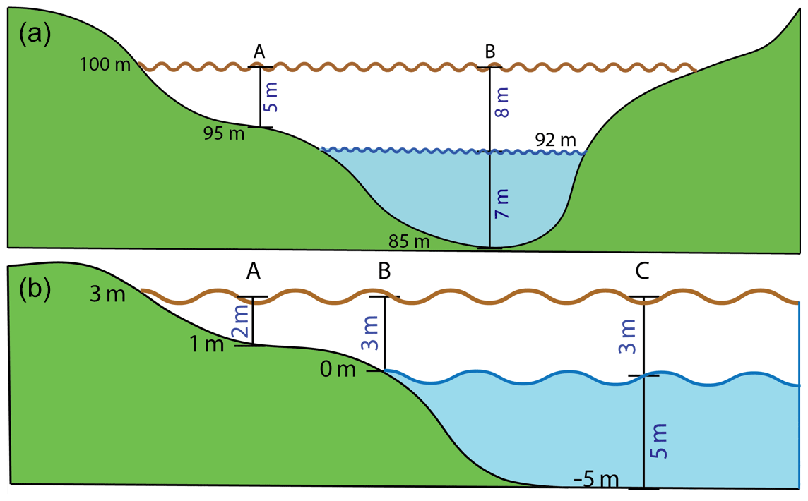
Figure 1Theoretical floodplain (a) and coastal (b) cross sections illustrating a FwDET floodwater depth calculation approach. The elevation (a.m.s.l.; black numbers) of the floodwater boundary (100 m at the top and 3 m in the bottom) are used to calculate water depth (blue numbers) for each grid cell within the flooded domain (point A). In riverine flooding (a) underestimation of water depth is expected over the river (point B) as DEMs typically capture the water surface elevation. In coastal flooding (bottom panel) the seaward flood boundary can be at the coastline (point B) or over the ocean (point C) and cannot be used to estimate floodwater depth (elevation ≤0). In FwDET v2.0 these boundary locations are excluded, which means that only the inland flood boundary is used.

Download

The first version of FwDET (v1.0) was implemented using a Python script, which utilizes ArcGIS tools (ArcPy library) for its core data analysis (available at https://sdml.ua.edu/models/, last access: 6 September 2019, and https://csdms.colorado.edu/wiki/Model:FwDET, last access: 6 September 2019). Floodwater elevation of the nearest boundary grid cell is allocated in FwDET v1.0 by iterating over increasing neighborhood sizes of the ArcGIS Focal Statistics tool (ESRI, 2019a). The iteration includes a condition to ensure newly allocated flooded grid cells receive elevation values from their closest computed neighbor (i.e., nearest boundary grid cell). This approach has three disadvantages: (1) it requires running the “Focal Statistics” tool multiple times, reducing FwDET computational efficiency; (2) the size of the largest neighborhood needed to cover the entire flooded domain varies depending on the domain size and the DEM resolution, requiring an a priori estimation of the number of iterations, often resulting in the need to rerun the tool; and (3) it ignores permanent water features (rivers, inlets), and thus can erroneously assign boundary grid cell elevations to flooded grid cells on the opposite bank because their Euclidian distance is shorter than to the boundary grid cells on their side of the waterbody.

In FwDET v2.0, allocation of the nearest boundary grid cell elevation is done with the ArcGIS “Cost Allocation” tool (ESRI, 2019b). Cost Allocation changes the way in which nearest boundary grid cells are allocated to a non-iterative approach. This drastically reduces the run time, as the tool uses one linear process to allocate the value of the input raster's (boundary elevation raster) nearest grid cell for all cells within the output domain. The tool's “cost” input raster is used in FwDET v2.0 to prevent boundary grid cell elevation allocation over permanent water by assigning such grid cells with high-cost value. The cost raster is calculated by assigning all grid cells with elevation equal to or less than zero a value of 1000 and all other grid cells a value of 1. For inland water bodies (e.g., rivers; where permanent water bodies have greater than zero elevation), a cost raster can be calculated from a land-cover map (through identification of permanent water bodies) and used as input to FwDET v2.0. The Cost Allocation tool only accepts integers, consequently creating a vertical elevation data resolution of 1 elevation unit (e.g., meter), which was the main reason this tool was not used in previous versions of FwDET. In FwDET v2.0, a float–integer–float conversion (multiplication of the DEM by 10⁶ and then dividing it by the same factor after the tool run) is employed to maintain the DEM vertical resolution.

FwDET v2.0 is also available as a Python script and as an ArcGIS script tool (see Conclusions section). A QGIS Python script and tool were developed to eliminate dependency on ArcGIS licensing. The QGIS script runtime is shorter than the ArcPy-dependent script but does not yet include a cost raster input and therefore does not solve the above-indicated issue of allocation across permanent water. It is therefore not a full solution of FwDET v2.0 but it does include the coastline boundary cell identification procedure.

2.2 Evaluation

FwDET v2.0 water depth estimations are evaluated here against calibrated hydrodynamic simulations. A similar approach was used in Cohen et al. (2018a) to evaluate FwDET v1.0. The flood extent used as input for FwDET v2.0 is derived from the modeled water depth rasters. The rasters were converted to FwDET inundation extent input polygons by reclassifying all nonzero water depth cells as 1 and using the ArcGIS “Raster to Polygon” tool to generate a feature layer. This allows for the evaluation of the FwDET v2.0 floodwater depth calculation approach without introducing potential biases by using different inundation extent data. The same DEMs were used for the model simulations and FwDET v2.0 calculation in each case study. The (calibrated) model-simulated water depth is assumed here to be the true water depth. Biases in this analysis are therefore solely a function of FwDET v2.0 algorithm results relative to the model's fluid dynamic simulation.

Two evaluation case studies are presented.

1. Portsmouth and Norfolk (Virginia, USA) includes coastal flooding in a relatively flat tidewater urban environment during Hurricane Irene in 2011. A 1 m topobathymetric lidar DEM, developed by Danielson et al. (2016), provided elevation inputs to two separate hydrodynamic models. These models operate at two different scales, large scale (20 m–10 km) to street-level scale (1–10 m). SCHISM (Semi-implicit Cross-scale Hydroscience Integrated System Model) covered half of the North Atlantic Ocean to the coastal zone with individual grid cells ranging from 20 m to 10 km. The UnTRIMV version 3 hydrodynamic model (Casulli, 2019) resolved an area the size of Portsmouth and Norfolk and their adjacent waterway systems at the street-level scale (1–10 m resolution grid, Wang et al., 2014). SCHISM is an open-source hydrodynamic model (Zhang et al., 2016), which provided tidal harmonic inputs at the open boundary and atmospheric inputs for Hurricane Irene from two different atmospheric model simulations. These atmospheric models were the Weather Research and Forecasting (WRF) model using nested 9, 3, and 1 km resolution grids, with hourly time intervals, and the European Centre for Medium-Range Weather Forecasts (ECMWF) model at 12 km resolution using 3 h time intervals. Water level outputs from SCHISM were used as Dirichlet open-boundary inputs for the street-level model to drive inundation into urban environments and highlight vulnerable infrastructure impacted during the storm. These urban structures were extracted from lidar as in Loftis and Taylor (2018) and directly embedded in the model to account for volume displacement within the structure's surface area and form drag as the storm surge flows around each building within the urban environment (Loftis et al., 2014, 2016). The street-level model subsequently generated hourly inundation outputs for floodwater depths in meters, which compared favorably with three municipally owned water level sensors (RMSE = 4.61 cm) and 18 USGS-reported high water marks (RMSE = 9.73 cm) in southeast Virginia, as noted in Loftis et al. (2018, 2019). A more complete description of this case study is available in Loftis et al. (2018) and Rogers et al. (2018). In this paper, the maximum water depth output was used along with the 1m DEM for the FwDET v2.0 calculation.

2. Brazos River (Texas, USA) riverine flooding during the May 2016 flood event. The same event was used to evaluate FwDET v1.0 and is used here to compare the two FwDET versions for riverine flooding. The iRIC-FaSTMECH hydrodynamics model (Nelson et al., 2016; https://www.i-ric.org, last access: 6 September 2019) was used to simulate the flood. The iRIC-FaSTMECH model simulates water velocity and water surface elevation using gauged discharge input at the reach's upstream location and stage at its downstream outlet. Manning's roughness parameter was calibrated, the pressure distribution was assumed hydrostatic, and the flow was considered quasi-steady in the model. A more detailed description of this case study is provided by Zhang et al. (2018) and Cohen et al. (2018a). In this paper, the maximum water depth model output along with the 10 m DEM (NED) were used for the FwDET v1.0 and v2.0 calculations.

2.3 Applications

Evaluation of FwDET v2.0 operational applications for three case studies is provided.

1. Hurricane Irene made landfall along the mid-Atlantic coast in late August 2011. To assess flooding from Irene, as part of the CAIR demonstration project, optical remote sensing approaches were used to map water extent, limited to views unobstructed by cloud, high objects like buildings, and vegetation. In this study, the highest-quality satellite overpass from Landsat was determined to be a Landsat 5 scene obtained on 31 August 2011, 5 d after the storm made landfall. To identify surface water areas, Landsat 5 surface reflectance was used to compute the modified normalized difference water index (mNDWI; Xu, 2006). Water detections from the Landsat 5 mNDWI product were then combined with the 2011 National Land Cover Dataset (NLCD) to separate flood areas from known permanent water locations. Areas that were identified as water in the mNDWI product and overlapped with identified water pixels in the NLCD were classified as persistent water. Pixels that were identified as water in mNDWI but not classified as water in the NLCD were determined to be flooded. Due to Landsat 5 imaging occurring after the initial landfall, the scene does not capture the maximum extent of flooding and omits significant flooding from a storm surge that had receded. A 30 m DEM (NED) was used as input for the FwDET v2.0.

2. Hurricane Florence made landfall in North Carolina on 14 September 2018. The slow-moving storm generated large amounts of rainfall over the Carolinas, resulting in widespread and severe riverine and pluvial flooding. GFP was activated on September 15. One of the products shared through the GFP network was a daily map of maximum detected flooding at 90 m resolution based on downscaled Advanced Microwave Scanning Radiometer 2 (AMSR2) and GPM Microwave Imager (GMI) passive microwave satellite observations from the Atmospheric and Environmental Research, Inc. (AER) FloodScan system (http://product.aer.com/index.php/floodscan/, last access: 6 September 2019). Whereas higher-resolution remote sensing products were shared by GFP members, the FloodScan maximum flooding product, which included flooding in woody wetland regions adjacent to observed floodwater, resulted in the most continuous and spatially extensive flood maps. A 30 m DEM (NED) was used for the FwDET v2.0.

3. In Sri Lanka torrential monsoon rainfall led to major flooding across the country in May 2018. GFP was activated on 22 May. As part of the GFP activation, the DFO Flood Observatory (hereafter DFO) published a flood map online based on 10 m resolution Sentinel-1b imagery (see DFO event page: http://floodobservatory.colorado.edu/Events/4619/2018Somalia4619.html, last access: 6 September 2019). Several DEM products were tested here as input for the FwDET v2.0 (described later).

3.1 FwDET v2.0 evaluation

Floodwater depth estimates by FwDET v2.0 correspond well with model-simulated water depth for the Norfolk–Portsmouth case study (Fig. 2). Maximum floodwater depth (the grid cell with the highest value) is overestimated by FwDET v2.0 but the water depth rasters yielded similar averages (0.77 and 0.65 m for the model and FwDET v2.0, respectively) and standard deviation (0.56 and 0.58 m for the model and FwDET v2.0, respectively). The mean difference in floodwater depths, calculated by averaging the raster values of the [FwDET v2.0 – model] map algebra expression, is −0.16 m with a standard deviation of 0.29 m, meaning that FwDET v2.0 slightly underestimates floodwater depth. The average absolute difference ([|(FwDET v2.0 − model)|]) is 0.18 m (23 % of the model mean average depth) with a standard deviation of 0.28 m. The histogram distribution (Fig. 2e) of the difference map (Fig. 2d) shows that the vast majority of grid cells have a bias of between 0 and −0.33 m and that biases below −1 m and above 0.33 m are rare.

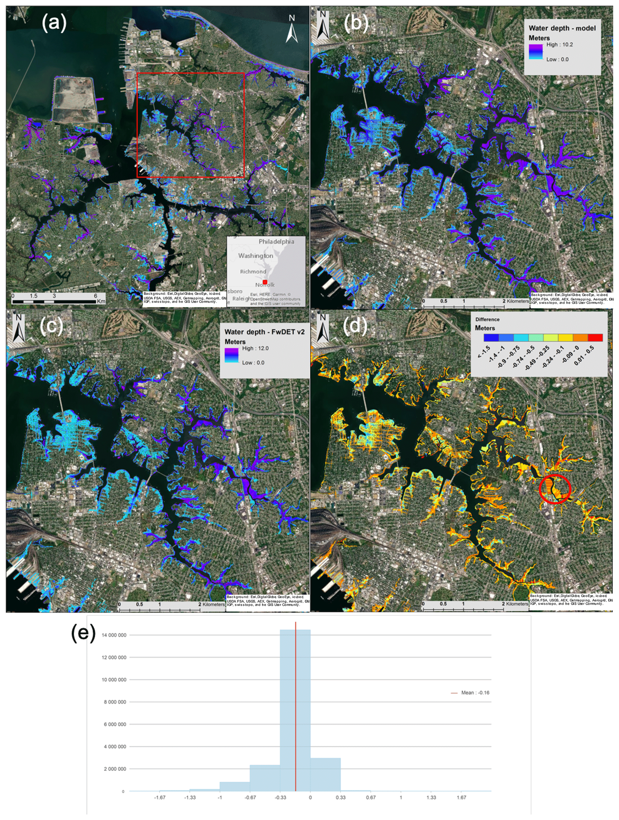
Figure 2The Norfolk–Portsmouth August 2011 Hurricane Irene flooding case study: (a) simulation domain, location overview map (bottom right inset), and the zoom-in extent used in panels (b)–(d) over the Lafayette River tidal estuary (red box); (b) model-simulated maximum water depth map; (c) FwDET v2.0 floodwater map; (d) difference map between panels (b) and (c) [FwDET v2.0 − model]; (e) histogram of grid cells in the difference map (d). Background sources: Esri, DigitalGlobe, GeoEye, i-cubed, USDA FSA, USGS, AEX, Getmapping, Aerogrid, IGN, IGP, swisstopo, and the GIS user community.

Although the mean difference in water depth estimations by FwDET v2.0 and the hydrodynamics model are small, the difference map (Fig. 2d) reveals a heterogenous tapestry of values, some of which are quite considerable and many with sharp (straight line) transitions, not readily apparent in the water depth maps (Fig. 2a and b). They are attributed to FwDET v2.0 reliance on nearest boundary cell elevation to calculate water depth. The use of Euclidian distance to assign the nearest boundary grid cell can lead to these straight-line transitions as well as inaccuracies in water depth where, for example, backwater effects are driven by complex flow paths. In urban environments, streets and buildings can amplify these biases. In this case study, in which a 1 m lidar DEM was used, buildings were identified as having a higher elevation. This created non-flooded areas within the flooded domain which FwDET v2.0 identified as boundary locations. Consequently, some nearby grid cells erroneously assigned values depicting unrealistic flood boundary elevations. These errors stem from false elevation reflections of sometimes multistory building roofs instead of the actual (street level) floodwater elevation. Similarly, other structures (e.g., highways, overpasses, dikes) can lead to these considerable overestimations. Effects of these are visible throughout Fig. 2d but are not consistent as some locations around buildings are actually underestimated. Underestimation by FwDET v2.0 is most common near banks and shorelines. This is due to the boundary grid cells assigned for these locations, which were not from the actual maximum inland extent of floodwater in that location, but of a nearer boundary grid cell which under-represents the true local floodwater elevation.

A comparison to FwDET 1.0 is not valuable for this (or any coastal) case study. This is because FwDET 1.0 does not work at coastal regions as the boundary elevation at the coastline is lower than the flooded domain. As a result, all the cells closest to the coastline (relative to the inland boundary) receive a no-data value.

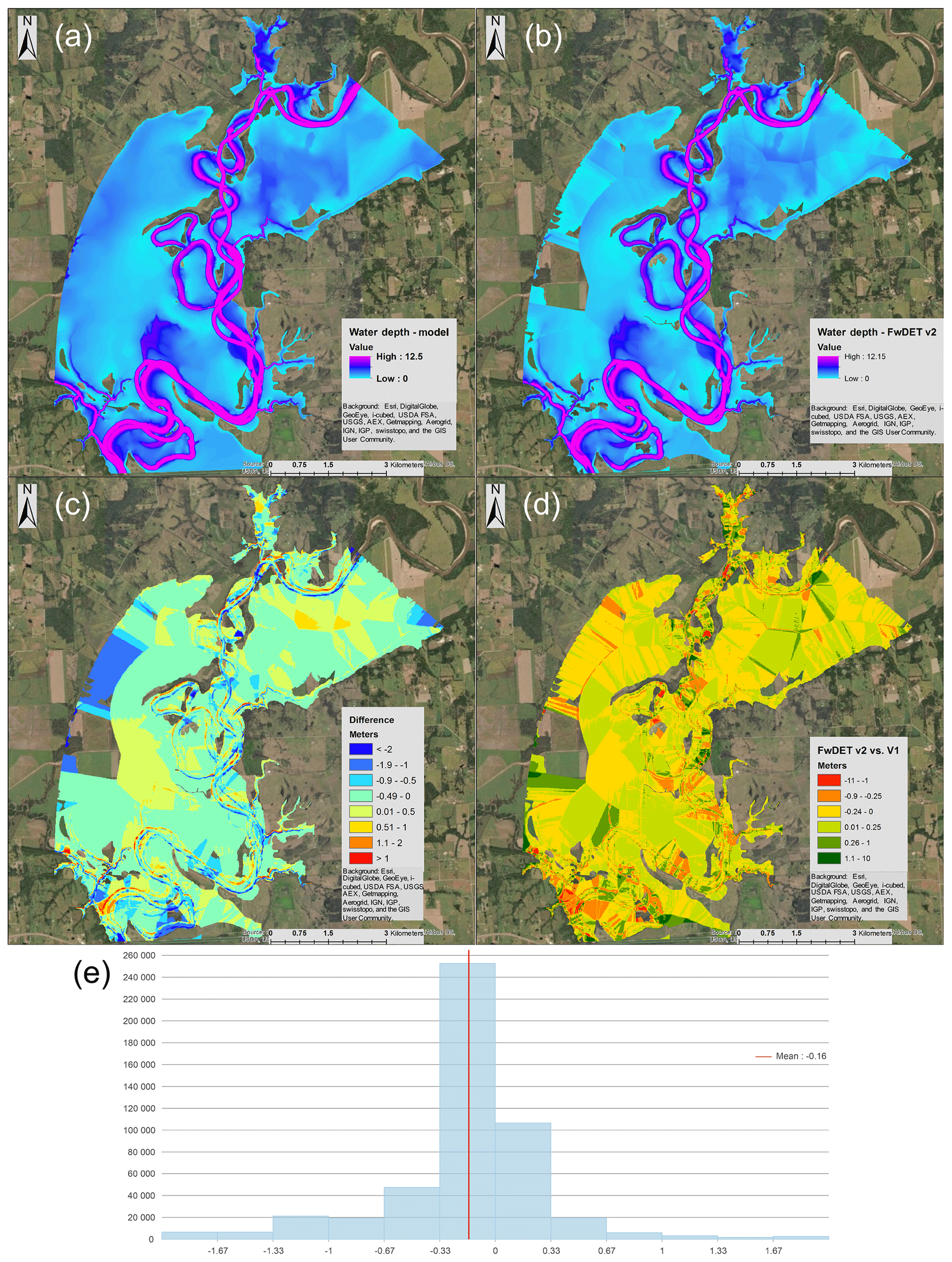
Figure 3The May 2016 flood event for the Brazos River (Texas) case study: (a) model-simulated maximum water depth; (b) FwDET v2.0 estimated floodwater depth; (c) difference map between panels (a) and (b) [FwDET v2.0 − model]; (d) comparison between FwDET v1.0 and v2.0 estimation accuracy [|v2.0 − model $|-|$ v1.0 − model|] (positive values indicate smaller bias by FwDET v2.0); (e) histogram of grid cell values of the difference map (c). Background sources: Esri, DigitalGlobe, GeoEye, i-cubed, USDA FSA, USGS, AEX, Getmapping, Aerogrid, IGN, IGP, swisstopo, and the GIS user community.

Floodwater depth estimates by FwDET v2.0 also correspond well with model-simulated water depth for the Brazos River case study (Fig. 3). Maximum water depths are similar (Fig. 3a and b). Average water depth calculated by FwDET v2.0 is 2.1 m, compared to the model's 2.2 m prediction. The standard deviation was also very similar with values of 2.51 m for FwDET v2.0 and 2.56 m for the model. The difference between the model and FwDET v2.0 water depth calculation is small with an average of −0.16 m [FwDET v2.0 − model] and a standard deviation of 0.46 m. Similar to the Norfolk–Portsmouth case study, FwDET v2.0 slightly underestimates floodwater depth. The absolute difference in water depth is 0.31 m (14 % of the model mean average depth) with a standard deviation of 0.46 m. The lower relative bias in the Brazos case study compared to the Norfolk–Portsmouth case study is likely due to the inclusion of the river itself in the statistical calculations. The river segment is relatively deep, and its water depth is relatively easy to estimate (not considering its true bathymetry). The histogram distribution (Fig. 3e) of the difference map (Fig. 3c) shows that the vast majority of grid cells have a bias of between −0.33 and 0.33 m with a small proportion of grid cells having a bias of over 1 and below −1.33 m.

The difference map (Fig. 3c) shows that the largest biases in FwDET v2.0 are mostly concentrated along the river channel. These are likely due to the hydraulic slope, which is simulated by the hydrodynamic model but are not expressed in the FwDET topography-based approach. As these biases relate to the active river channel, their implications for flood applications are small. Other regions of relatively high biases are along the western edges of the flooded domain. These are artifacts of the model domain setup. As described in Cohen et al. (2018a) and Zhang et al. (2018), the iRIC simulation grid extent and resolution must be manually defined by the user affecting the fluid dynamics along the edges of the simulation domain.

FwDET v2.0 shows a slight improvement over v1.0, which had a mean water depth of 1.95 m and an absolute difference of 0.37 m. A comparison of the two versions bias against the model results (Fig. 3d), calculated as [|FwDET v2.0 − model $|-|$ FwDET v1.0 − model|], has an average value of 0.01 m and standard deviation of 0.33 m. The differences between v1.0 and v2.0 are expected to be small for riverine flooding. The small improvement in FwDET v2.0 is primarily due to the use of a different tool for assigning the nearest boundary elevation (Focal Statistics loop in v1.0 vs. Cost Allocation in v2.0).

The Brazos River case study was also used to compare the runtime improvement of FwDET v2.0. At 10 m resolution the domain has 2087×1816 (3 789 992) grid cells requiring 100 iterations of the Focal Statistics loop in FwDET v1.0. FwDET v1.0, v2.0, and QGIS versions were run on a Windows 7 desktop with two Intel Xenon E5 2670 2.5 GHz processors and 64 GB of RAM. FwDET v1.0 runtime was 24 min and 14 s, FwDET v2.0 runtime was 1 min 33 s, and FwDET QGIS runtime was 49 s. This is a runtime improvement of over a factor of 15 between v1.0 and v2.0 and a further improvement by a factor of nearly 2 between v2.0 and QGIS. Faster runtime by FwDET QGIS is due to its use of GDAL's raster clipping tool, which is written in C (GDAL, 2019) and, similar to v2.0, there is no iterative loop. This clipping procedure (used in all FwDET versions) ensures that floodwater depth is rendered only within the flooded domain (see Cohen et al., 2018a). FwDET v2.0 ArcGIS script tool allows users to provide a pre-clipped DEM to reduce runtime. This is mostly useful when repeated runs for the same inundation extent are conducted.

3.2 FwDET v2.0 application results

Large-scale coastal flooding, typically associated with tropical cyclones, is challenging to analyze from both observational (remote sensing, point data) and modeling perspectives. This is because of the diversity in land cover and flooding sources. Storm surge, for example, can be highly energetic but short in duration relative to riverine flooding. That could create observational challenges for remote sensing applications. The NASA CAIR project (Rogers et al., 2018; NASA CAIR, 2018) utilized FwDET v2.0 to demonstrate the ability to integrate satellite-derived Earth observations and physical models into actionable knowledge. The integration of observations and models allows for a more comprehensive understanding of the compounding risk experienced in coastal regions. The demonstration produced flood inundation maps to predict building-level impacts of a representative storm in the mid-Atlantic region for Hurricane Irene. FwDET v2.0 used best-available remotely sensed imagery to determine inundation depth immediately following the storm.

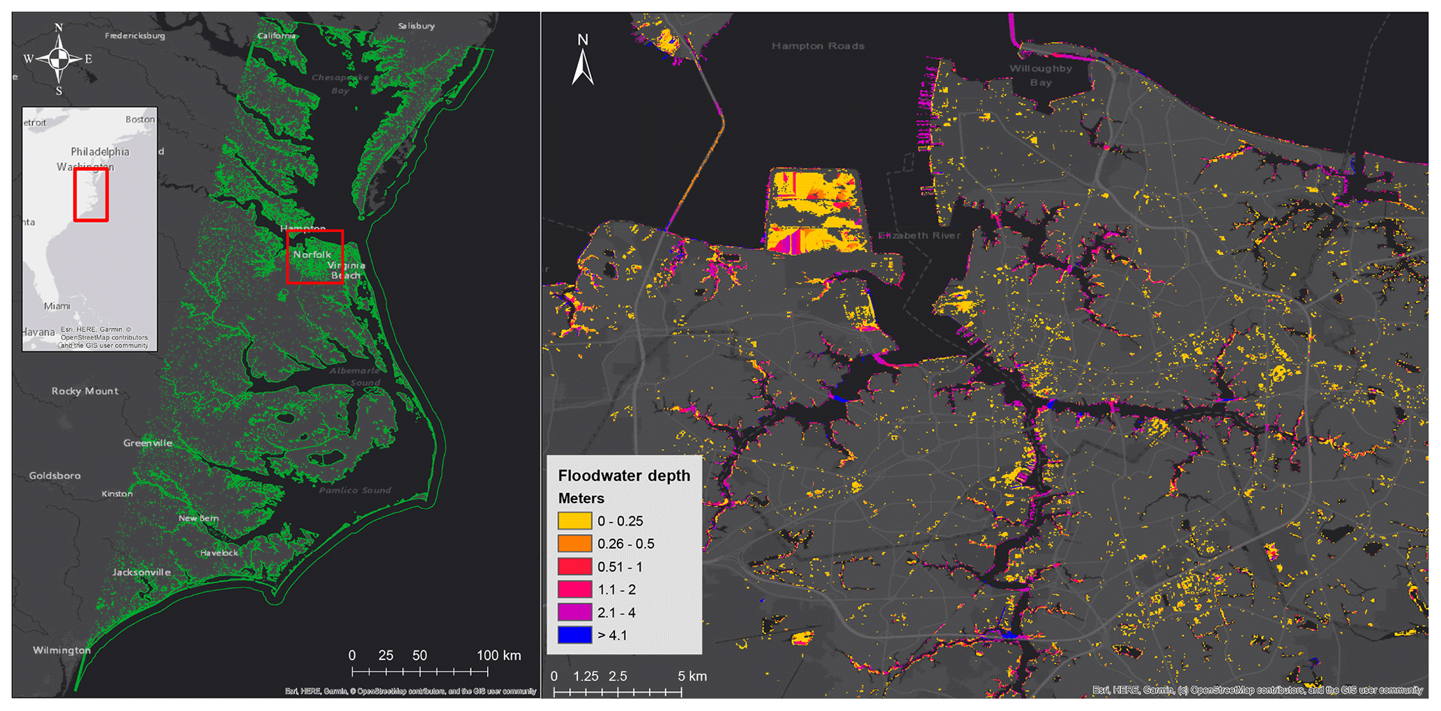
Figure 4Flooded domain and overview map (left panel) of the 2011 flooding following Hurricane Irene landfall on the US mid-Atlantic coast. The flood inundation was classified from two Landsat TM images which were used as input in FwDET v2.0 to calculate floodwater depth (right panel zooming-in on the Norfolk–Portsmouth area). Background sources: Esri, DeLorme, HERE, MapmyIndia. © OpenStreetMap contributors 2019. Distributed under a Creative Commons BY-SA License.

To estimate floodwater depth following Irene, the Landsat 5 floodwater classification was converted to a polygon layer (Fig. 4) to be used as input for FwDET v2.0. A DEM for the region was compiled by mosaicking the corresponding 30 m spatial resolution NED tiles. While 10 m NED products are available for this region, the 30 m product was used given the resolution of the flood inundation source (30 m Landsat 5 images) and the size of the domain (Fig. 4). Although there are insufficient ground-based observations to make a quantitative accuracy determination, overall the spatial trends in water depth estimation seem reasonable. The average floodwater depth for the entire domain was 0.64 m with a maximum of 41.7 m. The latter is obviously an overprediction resulting from the misclassification of floodwater from the satellite imagery or spatial mismatch between the inundation map and the DEM. Zooming in on the Norfolk–Portsmouth area reveals (Fig. 4 right panel) a much smaller flooding extent compared to the model simulation results (Fig. 2). This is reasonable given that the model simulated the maximum flooding conditions during the event while the flood inundation layer used here is based on a Landsat 5 image captured 5 d past the hurricane's landfall. Underprediction of flood extent may also be due to challenges in floodwater classification in urban environments at this resolution. Average floodwater depth calculated by FwDET v2.0 for the Norfolk–Portsmouth domain was 0.85 m, which is slightly higher than water depth predictions for the same domain in the high-resolution maximum-extent case study (Fig. 2; 0.77 and 0.65 m for the model and FwDET v2.0, respectively). The likely cause for this overestimation in this coastal urban region is the resolution of the inundation map and DEM relative to the area's small topographic gradient and fragmentation of the flooded domain. Thus, the use of FwDET v2.0 over large coastal flood domains can be useful for providing a synoptic overview of flood severity, but its localized analysis, especially for urban areas, should be considered in the context of the input data used (mainly its resolution).

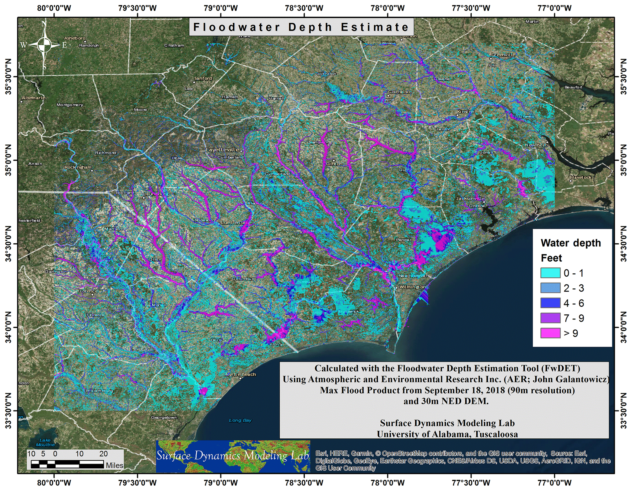
Figure 5A floodwater depth map which was shared during the GFP Hurricane Florence activation. Water depth was calculated with FwDET v2.0 using a maximum inundation extent map (as of 18 September 2018) and a 30 m DEM (NED). Units were converted to US customary units for better integration in US emergency response entities. Background sources: Esri, DigitalGlobe, GeoEye, i-cubed, USDA FSA, USGS, AEX, Getmapping, Aerogrid, IGN, IGP, swisstopo, and the GIS user community. © OpenStreetMap contributors 2019. Distributed under a Creative Commons BY-SA License.

For the Hurricane Florence application case study, FwDET v2.0 estimates (Fig. 5) show high water depths (over 3 m) within the major river floodplains and shallow to medium water depths (below 3 m) across the flooded domain. Average floodwater depth is 0.92 m with a standard deviation of 1.7 m. This is a reasonable result given the other case studies (we do not have comprehensive observed or simulated water depth data for a quantitative assessment). Maximum estimated water depth is 39.6 m, which is clearly an overestimation, even though calculations include permanent water features. That is because DEMs typically capture the water surface elevation of permanent water features (see Fig. 1).

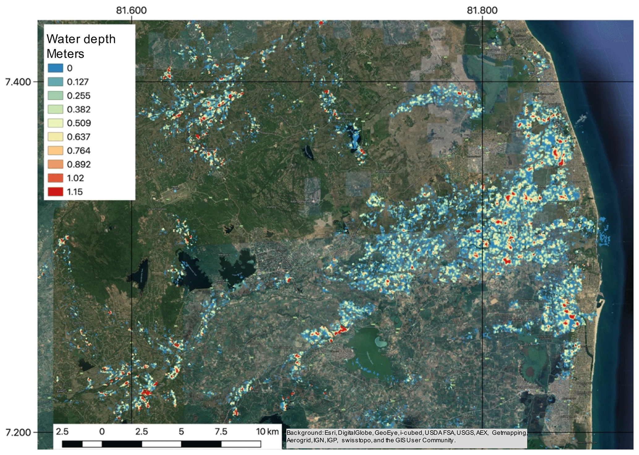
Figure 6A floodwater depth map shared during the GFP activation for the 2018 flooding in Sri Lanka, zooming in on the southeast part of the country. Water depth was calculated using FwDET v2.0 with a 10 m flood inundation map (for 19 May 2018) and 30 m DEM (ALOS). Background sources: Esri, DigitalGlobe, GeoEye, i-cubed, USDA FSA, USGS, AEX, Getmapping, Aerogrid, IGN, IGP, swisstopo, and the GIS user community.

For the Sri Lankan application case study, the flood inundation map produced by DFO was highly fragmented in most parts of the country leading to many small inundation polygons (Fig. 6). The remote sensing classification used appears to be an accurate representation of ground conditions given the sensor resolution. As described earlier, fragments in the inundation extent, assuming it represents reality, can be advantageous as it can shorten the distance to the nearest boundary grid cells, which may yield more accurate (localized) water elevation estimation by FwDET v2.0. However, a highly fragmented inundation extent can be problematic if the flooded sections are small relative to the input DEM resolution and the local terrain gradient. For example, a flooded area with an extent of only a few DEM grid cells in a flat area may result in a negligible water depth because the elevations of the boundary and inundated grid cells are similar. High-resolution DEMs outside the US are often difficult to obtain as most countries do not openly share national DEMs, or they do not exist. As a result, in emergency response situations, we often can only use global DEMs as input to FwDET (see Cohen et al., 2018a, b). For this event three DEM products were tested:

1. HydroSHEDS (based on the Shuttle Radar Topography Mission (SRTM) DEM); 3 arcsec (∼90 m) resolution.

2. Multi-Error Improved–Terrain (MERIT; Yamazaki et al., 2017); 3 arcsec (∼90 m) resolution; http://hydro.iis.u-tokyo.ac.jp/~yamadai/MERIT_DEM/index.html (last access: 6 September 2019).

3. ALOS; 30 m resolution; http://www.eorc.jaxa.jp/ALOS/en/aw3d30/index.htm (last access: 6 September 2019).

While ALOS offers the highest spatial resolution, it is distributed as an integer raster, which means that its vertical resolution is effectively 1 m. This is a considerable disadvantage, especially in low slope terrains. MERIT resulted in improved depth estimations over using HydroSHEDS (not shown here) but its horizontal resolution is inadequate considering the resolution of the remote sensing inundation map (10 m) and the high degree of fragmentation in the inundation extent input. Use of the ALOS DEM yielded the most appropriate floodwater depth map (Fig. 6) for the Sri Lankan flood, but with a relatively high degree of uncertainty due to its limited vertical resolution, a high degree of fragmentation relative to the DEM vertical resolution, and mismatch in horizontal resolution between the inundation map and DEM. This event demonstrated challenges associated with high-resolution DEM availability. This case study highlights the need to carefully consider the appropriateness of DEM choice in the context of the resolution and nature of the inundation extent map.