the Creative Commons Attribution 4.0 License.
the Creative Commons Attribution 4.0 License.
 | 12 Nov 2019
Reconstructing patterns of coastal risk in space and time along the US Atlantic coast, 1970–2016
Scott B. Armstrong
Despite interventions intended to reduce impacts of coastal hazards, the risk of damage along the US Atlantic coast continues to rise. This reflects a long-standing paradox in disaster science: even as physical and social insights into disaster events improve, the economic costs of disasters keep growing. Risk can be expressed as a function of three components: hazard, exposure, and vulnerability. Risk may be driven up by coastal hazards intensifying with climate change, or by increased exposure of people and infrastructure in hazard zones. But risk may also increase because of interactions, or feedbacks, between hazard, exposure, and vulnerability. Using empirical records of shoreline change, valuation of owner-occupied housing, and beach-nourishment projects to represent hazard, exposure, and vulnerability, here we present a data-driven model that describes trajectories of risk at the county scale along the US Atlantic coast over the past 5 decades. We also investigate quantitative relationships between risk components that help explain these trajectories. We find higher property exposure in counties where hazard from shoreline change has appeared to reverse from high historical rates of shoreline erosion to low rates in recent decades. Moreover, exposure has increased more in counties that have practised beach nourishment intensively. The spatio-temporal relationships that we show between exposure and hazard, and between exposure and vulnerability, indicate a feedback between coastal development and beach nourishment that exemplifies the “safe development paradox”, in which hazard protections encourage further development in places prone to hazard impacts. Our findings suggest that spatially explicit modelling efforts to predict future coastal risk need to address feedbacks between hazard, exposure, and vulnerability to capture emergent patterns of risk in space and time.
- Article
(2537 KB) -
Supplement
(1145 KB) - BibTeX
- EndNote


Risk reduction in developed coastal zones is a global challenge (Parris et al., 2012; Sallenger et al., 2012; Witze, 2018; Wong et al., 2014). Risk can be expressed as a function of hazard, exposure, and vulnerability. In the terminology of the US National Research Council (NRC, 2014; Samuels and Gouldby, 2005), hazard is typically expressed as the likelihood that a natural hazard event will occur (e.g. a recurrence interval for a storm of a given magnitude) or as a chronic rate of environmental forcing (e.g. a rate of sea-level rise). Exposure tends to capture either the economic value of property and infrastructure that a hazard could negatively impact or the number of people a hazard could affect. Vulnerability can reflect a wide variety of dimensions, but in physical terms (relative to social metrics) vulnerability generally represents the susceptibility of exposed property to potential damage by a hazard event (NRC, 2014). Although the reduction of disaster risk – across all environments, not only coastal settings – is an intergovernmental priority (UNISDR, 2015), a paradox has troubled disaster research for decades. Even as scientific insight into physical and societal dimensions of disaster events become clearer and more nuanced, the economic cost of disasters keeps rising (Blake et al., 2011; Mileti, 1999; Pielke Jr. et al., 2008; Union of Concerned Scientists, 2018).
There are a number of possible explanations for this trend. Economic costs could be rising because natural hazards, exacerbated by climate change, are getting worse (Estrada et al., 2015; Sallenger et al., 2012); because with migration and population growth more people are living in hazard zones (NOAA, 2013); or because more infrastructure of economic value, from highways to houses, now exists in hazard zones (AIR Worldwide, 2016; Desilver, 2015; Union of Concerned Scientists, 2018). These drivers are typically addressed separately – but they are not mutually exclusive. A parallel explanation for the disaster paradox is that environmental, population, and infrastructural drivers are systemically intertwined, resulting in “disasters by design” (Mileti, 1999) – unintended consequences of coupled interactions, or feedbacks, between natural forcing and societal shaping of the built environment. An example of one such feedback is when infrastructure development in hazard zones destroys natural features that would otherwise buffer hazard impacts, such as the loss of coastal wetlands that would have absorbed storm surge (Barbier et al., 2011; Arkema et al., 2013; Temmerman et al., 2013). An example of another feedback is when hazard defences stimulate further infrastructure development behind them – a phenomenon called the “land-use-management paradox”, “levee effect” or “levee paradox”, or the “safe development paradox” (Armstrong et al., 2016; Burby and French, 1981; Burby, 2006; Di Baldassarre et al., 2016; Keeler et al., 2018; McNamara and Lazarus, 2018; Werner and McNamara, 2007; White, 1945). While both feedbacks can increase hazard impacts without any change in natural forcing, climate change accelerates them.
Investigations of coastal risk tend to focus on case studies of hazard, exposure, and/or vulnerability (Smallegan et al., 2016; Taylor et al., 2015), or on projections of future risk (e.g. Brown et al., 2016; Hinkel et al., 2010; Neumann et al., 2015). Few examine patterns of risk across large spatial scales (∼102–103 km) or retrospectively over longer timescales (>101 yr). Here, we develop a data-driven model to investigate how hazard, exposure, and vulnerability may describe trajectories of risk in space and time along the US Atlantic coast, from Massachusetts to southern Florida, at the county level for the past 47 years (Fig. 1). We restrict our analysis of risk to three specific components: shoreline change (hazard), valuation of owner-occupied housing units (exposure), and beach nourishment – the active, and typically repeated, placement of sand on a beach to counteract chronic erosion (vulnerability). We do not address socioeconomic or demographic exposure or vulnerability (Cutter and Emrich, 2006; Cutter and Finch, 2008; Cutter et al., 2006, 2008) nor the exposure of infrastructural aspects of the built environment beyond owner-occupied housing value. We also do not address other types of coastal hazard, such as storm strikes or flooding, or types of hazard mitigation other than beach nourishment. Despite this tightly defined framing, our analysis captures underlying quantitative relationships between risk components. Our findings suggest that spatially explicit modelling efforts to predict future coastal risk need to address feedbacks between hazard, exposure, and vulnerability to capture emergent patterns of risk in space and time.
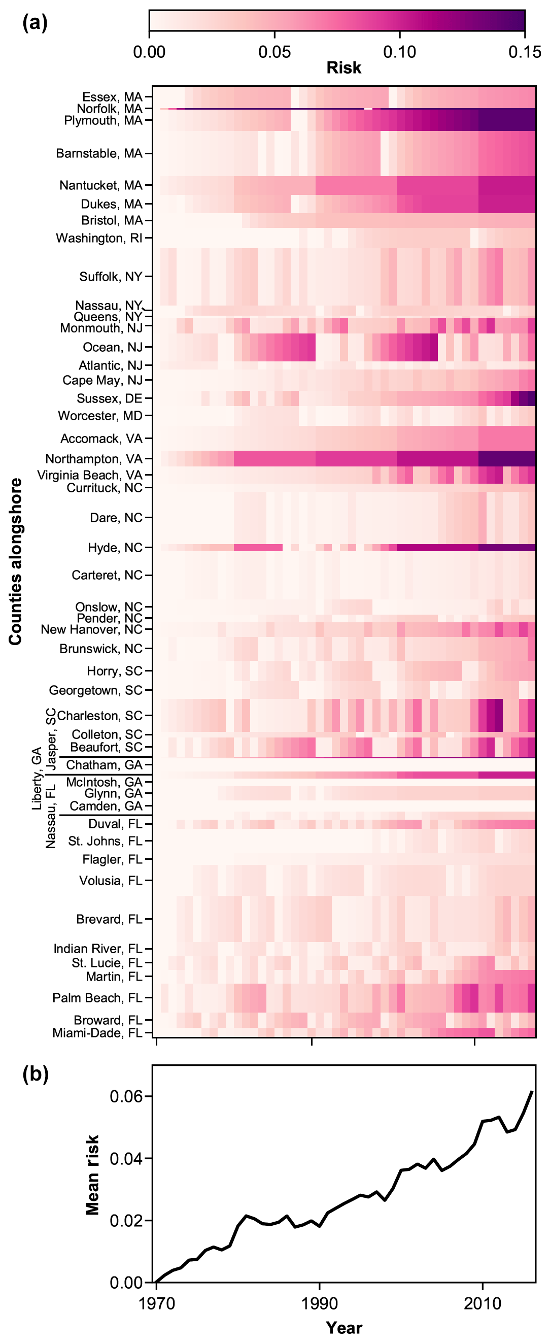
Figure 1Evolution of (a) county-level risk (a function of hazard, exposure, and vulnerability) modelled for the US Atlantic coast, from 1970 to 2016. Hazard in this simulation reflects historical erosion rates. For visualization and analysis, each county is scaled by the number of 1 km transects it comprises. The result is a matrix of 2386 km over 47 years, in which each of the 2386 (1 km) rows is associated with a county. Note that risk in Norfolk County, MA, exceeds the maximum scale bar value of 0.15 (2016 risk = 0.418; see Table 1). (b) Alongshore mean values through time for the whole US Atlantic coast are taken from the full matrix (a), reflecting the relative alongshore scale of each county.
Using the components of risk broadly defined by the US National Research Council (NRC, 2014; Samuels and Gouldby, 2005), we represent coastal risk as a function of time (t) with the expression
where R is coastal risk, H is natural hazard, E is exposure, and V is vulnerability. We define hazard (H) in terms of chronic shoreline erosion (as opposed to the likelihood of a hazard event). We define exposure (E) in terms of the total property value of owner-occupied housing units in 51 US Atlantic coastal (ocean-facing) counties. We address vulnerability (V) as a function of beach width, modulated by beach nourishment, which functions as a buffer between hazard and exposure (Armstrong and Lazarus, 2019; Armstrong et al., 2016).
2.1 Hazard
We calculated rates of shoreline change in two different ways to compare their respective effects on risk over time.
2.1.1 Shoreline-change rates from shoreline surveys
First, we calculated “end-point” rates of change from surveys of shoreline position published by the US Geological Survey (USGS) (Himmelstoss et al., 2010; Miller et al., 2005). An end-point rate is the cross-shore distance between two surveyed shoreline positions, divided by the time interval between the surveys. Using the Digital Shoreline Analysis System (DSAS) tool for ArcGIS (Thieler et al., 2008), we cast cross-shore transects every 1 km alongshore to intersect the surveyed shorelines, and at each transect calculated the end-point rate for three time periods (Armstrong and Lazarus, 2019): “historical”, from the first survey to 1960; “recent”, from 1960 to the most recent survey; and “long-term”, from the first survey to most recent (Figs. 2a, e, i and 3a). Because the dates of shoreline surveys vary by location, following Armstrong and Lazarus (2019) we calculate shoreline-change rates using the available surveys at each transect that are closest to the start and end dates of each period. We calculated the median historical, recent, and long-term rates of shoreline change for each county alongshore.

Figure 2Columns show hazard, exposure, and vulnerability components and resulting risk. Each row of panels illustrates a different rate of shoreline change (i.e. hazard condition): (a–d) historical, (e–h) recent, and (i–l) long term. Risk in Norfolk County, MA, exceeds the maximum scale bar value of 0.15 (2016 risk = 0.418; see Table 1). Each county is scaled by the number of 1 km transects it comprises; the northern- and southernmost counties are labelled.
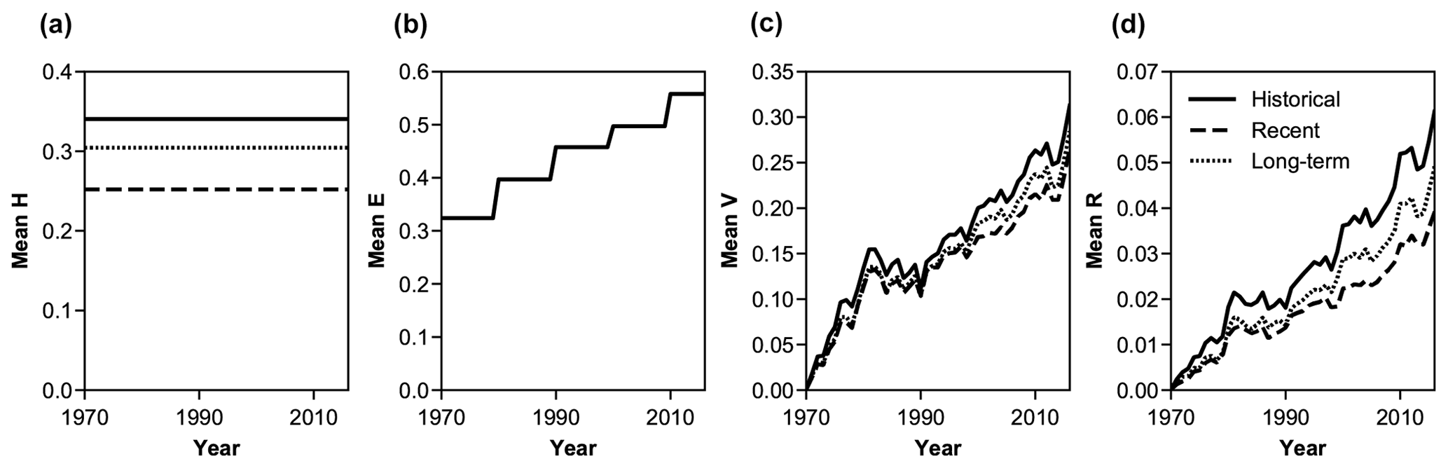
Figure 3Evolution over time of alongshore mean risk components – (a) hazard, (b) exposure, and (c) vulnerability – and the resulting (d) mean risk, given historical (solid black), recent (dashed black), and long-term (dotted black) shoreline-change rates as hazard conditions.
We used 1960 to differentiate between historical and recent shoreline-change rates because during that decade beach nourishment overtook shoreline hardening to become the predominant form of coastal protection in the United States (NRC, 1995, 2014). Cumulative, diffuse effects of nourishment are therefore embedded in recent and long-term rates of shoreline change (Hapke et al., 2013; Johnson et al., 2015). We report long-term end-point rates for context because they are common in other shoreline-change studies, particularly for the US mid-Atlantic region (Hapke et al., 2013). However, a historical rate calculated from shorelines surveyed prior to 1960 may better reflect environmental forcing in the effective absence of beach nourishment (Armstrong and Lazarus, 2019). Historical rates are not “natural” rates: human alterations to the US Atlantic coast began long before 1960, with engineered protection, including seawalls, groyne fields, and limited beach-nourishment projects (Hapke et al., 2013). Here, we consider them a pre-nourishment “background” rate of chronic forcing.
2.1.2 Shoreline-change rates from sea-level change rates
To test an independent measure of chronic shoreline-change hazard, we also derived rates of shoreline change (Fig. 4a and e) from recorded rates of sea-level change (Holgate et al., 2013; PSMSL, 2018) and a USGS dataset of cross-shore slope for the US Atlantic coast (Doran et al., 2017). We calculated spatially distributed rates of sea-level rise from annual tide-gauge records maintained by the Permanent Service for Mean Sea Level (PSMSL) (Holgate et al., 2013; PSMSL, 2018). For each tide-gauge record, we linearly interpolated across gaps in the annual data. We smoothed the resulting continuous record with a 10-year moving average and calculated the annual rate of sea-level change (Table S1 in the Supplement). Because the tide-gauge locations are not evenly distributed alongshore, to find rates of sea-level change for the full extent of the US Atlantic coast we linearly interpolated rates of sea-level change between tide-gauge stations, and we calculated the median annual rate of sea-level change at each coastal county. To convert a vertical change in sea level to a horizontal change in shoreline position, we shifted shoreline position at each transect up (or down) the cross-shore slope from USGS coastal lidar surveys (Doran et al., 2017) (Table S2). Linking the slope measurements to county shapefiles with a spatial join, we calculated median slope per county and then the horizontal distance that each annual vertical change in sea level moved the shoreline (Fig. 4a).
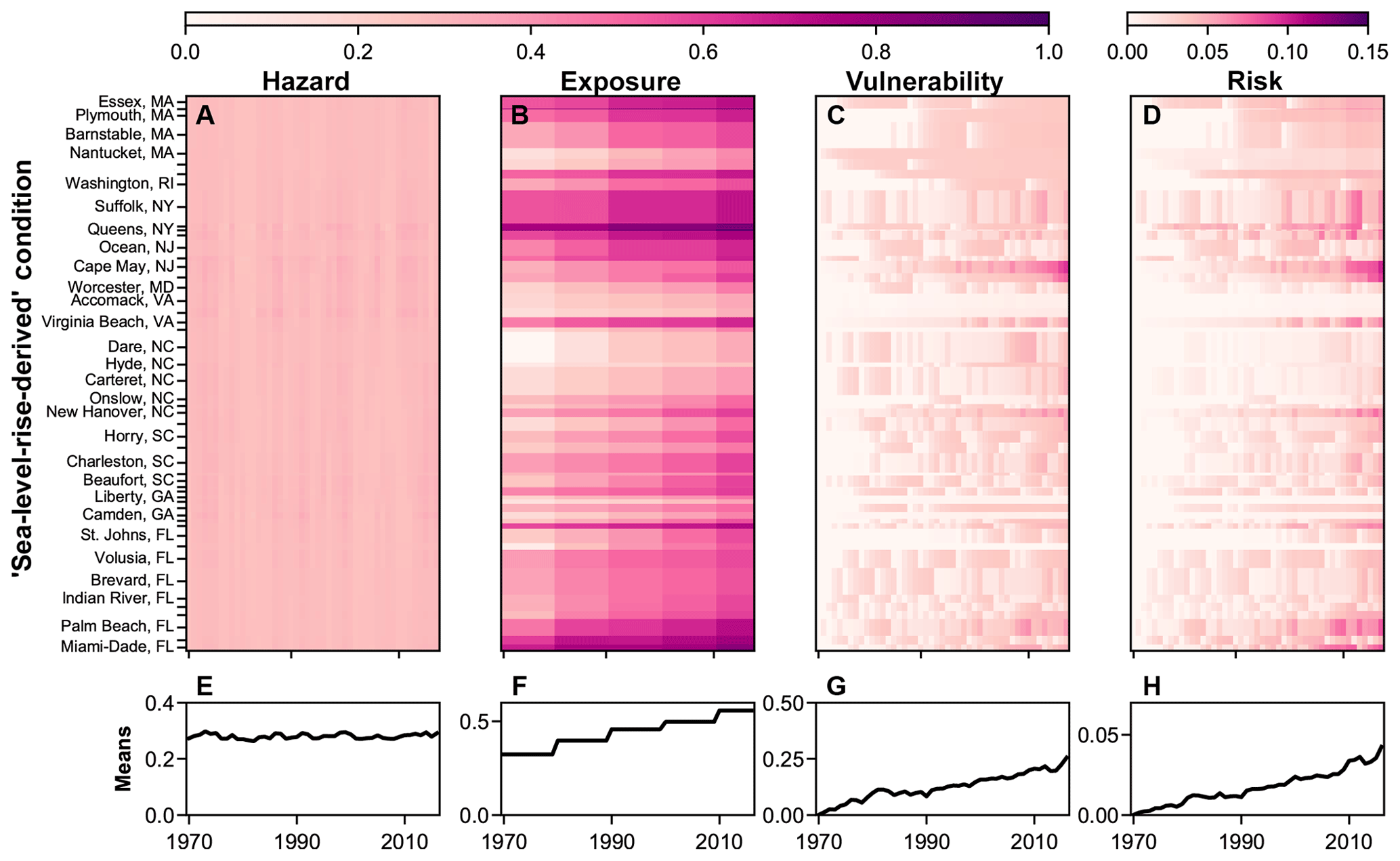
Figure 4County-scale component (a) hazard, (b) exposure, (c) vulnerability, and (d) overall risk evolution over time and (e–h) corresponding means, using shoreline-change rates derived from sea-level change as the hazard condition. Each county is scaled by the number of 1 km transects it comprises; not all counties are labelled.
The relationship between sea-level change and shoreline position is more complicated than the one abstracted in our deliberate simplification (Cooper and Pilkey, 2004; Lentz et al., 2016; Nicholls and Cazenave, 2010). Our estimation is effectively a “bathtub model” of change, controlled only by topography with no incorporation of wave-driven sediment transport or other shoreline dynamics. Bathtub models tend to underpredict shoreline erosion rates in wave-dominated, sandy barrier settings, such as those of the US mid-Atlantic (Lorenzo-Trueba and Ashton, 2014; Wolinsky and Murray, 2009). However, for this exercise, our method is useful for its simplicity – especially given the spatial scales under consideration – and for the independent estimation of shoreline change that it provides.
2.1.3 Sign convention
By the sign convention in our calculations, a negative rate of shoreline change denotes accretion (reducing hazard), and a positive rate denotes erosion (increasing hazard) (Fig. 2a, e, and i). Hazard magnitudes are normalized by the minimum and maximum rates to range between 0 and 1.
2.2 Exposure
To represent exposure along the US Atlantic coast, we used county-level census data for the total value (adjusted to 2018 US dollars) of owner-occupied housing units in 51 coastal (ocean-facing) counties for each decade since 1970 (Table S3) (Minnesota Population Center, 2011). Because property value data are sparse for the 2010 census community survey (16 Atlantic coastal counties are missing), we instead used the 2009–2013 census 5-year survey. Several 5-year census surveys incorporate 2010, but we chose the 2009–2013 survey because it provides full coverage of all the Atlantic coastal counties, and its mean of total values is closest to the 2010 census community survey (for those Atlantic coastal counties surveyed in 2010). We adjusted the county-total values of owner-occupied housing units to 2018 US dollars and divided by the number of transects in each county to yield a proxy for property value per alongshore kilometre. Because of the range of values along the coast, we took a log-transform and normalized the results to fall between 0 and 1 (Figs. 2b, f, j and 3b).
2.3 Vulnerability
We represented vulnerability (V) with a two-part relationship based on beach width (Vbw) and beach nourishment (Vbn) over time:
Because the value of exposed property is not included in Vbw or Vbn, this formulation disentangles vulnerability from exposure – a subtle but important conceptual departure from the definition used by the National Research Council (NRC, 2014; Samuels and Gouldby, 2005), which includes property values in vulnerability.
We made the beach-width component (Vbw) inversely related to beach width, such that vulnerability increases as beach width decreases. We express the normalized beach-width component as
where x0 is maximum beach width, xmin is minimum beach width, and x is beach width. Because real measurements are unavailable, we assumed that in 1970 all counties had the same initial beach width. (In the results presented here, xmin=10 m and x0=50 m; see also Table S4.) From this baseline, the county-scale shoreline erodes or accretes according to the linear rate determined by the hazard condition (historical, recent, long term, or derived from sea level). Because we used counties as the smallest spatial unit of comparison, our assumption implies that each county is fronted by beach. The physical geography of the real coastline is, of course, more spatially heterogeneous. Our analysis is too coarse to capture, for example, change at isolated pocket beaches in a predominantly rocky coastline, but counties with rocky coastlines will reflect very low or null rates of shoreline change. We consider only oceanfront shoreline, and we do not account for back-bay or estuarine shoreline.
For the beach-nourishment factor (Vbn), we collated beach-nourishment projects since 1970 by county from the beach-nourishment database maintained by the Program for the Study of Developed Shorelines (PSDS, 2017). We took Vbn as the running total number of nourishment projects per county (nc) over time (t, summed annually), and we normalized Vbn by the maximum number of projects among counties as of 2016 (), such that the county that nourished the most has Vbn=1 in 2016. Each county starts with Vbn=0 in 1970, and Vbn increases incrementally with every nourishment project within the county boundary:
We initiated Vbn in 1970 to match the census data for exposure (E). Because 80 % of beach-nourishment projects on the US Atlantic coast have occurred since 1970, we excluded a relatively small number of events. To test the sensitivity of our vulnerability and risk results to the 1970 start date, we examined the relative effects of (1) initiating Vbn from the first nourishment project in our record (in 1930) and (2) excluding the Vbn term altogether (Fig. S1 in the Supplement). Although the risk patterns resulting from these sensitivity tests changed in detail, their general characteristics did not.
In our routine, until a county nourishes for the first time, beach width (x) changes according to the county median linear erosion rate (γ):
The linear erosion rate (γ) applied to each county is either the (pre-normalized) historical, recent, or long-term shoreline-change rate or the rate derived from sea-level change, depending on the hazard scenario. The sign convention for γ is negative for erosion and positive for accretion.
Once a county has nourished – as determined by the empirical dataset of nourishment projects (PSDS, 2017) – beach width becomes a function of a linear erosion rate (γ), as in Eq. (5), and a nonlinear erosion rate (θ), which is applied to the nourished fraction of the total beach width (μ) to capture cross-shore and alongshore diffusion of nourishment deposition across and along the shoreface (Dean and Dalrymple, 2001; Lazarus et al., 2011; Smith et al., 2009):
where x0 is maximum beach width, θ is nonlinear erosion rate, μ is the fraction of the total beach width that the nonlinear rate applies to, γ is linear erosion rate, and t is the number of years since the last nourishment project. If a county nourishes at least once in a given year, its beach is restored to a maximum width in that year before it begins to erode. (Our minimum temporal increment was 1 year, and we assumed that nourishment always occurs at the end of a given year.) Maximum beach width (x0), nonlinear erosion rate (θ), and the fraction of beach width affected by the nonlinear rate (μ) are variables applied to the full spatial domain. Beach width (at the county scale) thus changes at a linear rate (γ), where a negative value is erosion and a positive value is accretion, with an additional nonlinear erosion rate (θ) over a fraction of the beach (μ) when nourishment occurs, until the beach is restored to maximum width by a subsequent nourishment project or reaches a specified minimum width (here 10 m). The Vbn term is ultimately normalized by the maximum and minimum beach widths.
Because vulnerability is normalized, the minimum beach width that we specify (xmin=10 m) affects the length of time it takes to reach maximum Vbw but does not affect the overall magnitude of V. A wider minimum threshold means that Vbw reaches a maximum faster, and vice versa. We used a minimum width of 10 m to avoid the numerical instabilities in Vbw that arise with a minimum width equal to or less than 0 m. The minimum width threshold does not affect the cumulative beach-nourishment factor.
We test the effect of altering x0, θ, and μ on both vulnerability and risk, under historical hazard and linear erosion rates (Fig. S1; Table S4). Sensitivity testing shows that vulnerability over time is highest in the case of a narrow beach (x0=25 m) with a high nonlinear erosion rate (θ=0.75) affecting a large fraction of the beach (μ=0.75). Vulnerability over time is lowest in the opposite case (x0=100 m, θ=0.05, μ=0.25) (Fig. S1). In calculating our results, we used a case in the middle of these extremes (x0=50 m, θ=0.5, μ=0.33), applying a value of μ similar to the value (μ=0.35) used by Smith et al. (2009) and Lazarus et al. (2011).
Like a ratchet, the cumulative beach-nourishment factor (Vbn) increases each time a county nourishes. This assumption represents the fact that nourishment projects for shoreline protection (as opposed to reactionary projects for emergency storm response) are cyclical within multi-decadal programmes (NRC, 1995, 2014). Nourishment at a given site rarely occurs only once. A community that initiates a nourishment programme will likely depend on periodic nourishment into the future. By comparison, the beach-width factor (Vbw) is more dynamic, reflecting the oscillatory behaviour of a nourishment cycle at multi-annual timescales by dropping to a minimum after a nourishment project (as the wide beach buffers property from hazard) and then increasing as the nourished beach erodes and coastal properties become more susceptible to hazard.
2.4 Statistical tests
We examine relationships between the resulting spatial distributions of hazard, exposure, and vulnerability over time using a Kolmogorov–Smirnov test that quantifies, to 95 % confidence, relative differences between pairs of distributions. A Kolmogorov–Smirnov test does not require parametric distributions, and it evaluates the null hypothesis that a given pair of distributions are sampled from the same parent distribution. Rejection of the null hypothesis thus means the distributions are significantly different.
3.1 Risk trajectories
Our data-driven model generates a pattern of coastal risk that varies in space and time at the county scale along the US Atlantic coast (Fig. 1). From 1970, each county generates its own risk trajectory that represents the interaction of hazard, exposure, and vulnerability in that county (Fig. 1a). For visualization and analysis, we scaled each county by the number of 1 km transects they comprise (Fig. 1a). The result is a matrix of 2386 km over 47 years, in which each of the 2386 (1 km) rows is associated with a county. Alongshore mean values for the whole US Atlantic coast are taken from the full matrix so that they reflect the relative alongshore scale of each county (Fig. 1b).
We find that the collective trajectory of risk increases from 1970 to 2016 for all hazard scenarios – despite the occurrence of 998 beach-nourishment projects, ostensibly intended to reduce risk, during the same period (Figs. 2 and 3). The influence of beach-nourishment projects on vulnerability means that county-scale risk varies over time even if hazard forcing remains constant. Because hazard based on measured shoreline change (historical, recent, and long term) is spatially variable but temporally static (Figs. 2 and 3), changes in risk over time under this model condition are driven by either exposure or vulnerability.
The overall risk trajectory also increases with the spatio-temporally variable hazard condition derived from rates of sea-level rise (Fig. 4). The alongshore mean rate derived from sea-level rise shows close agreement with the mean recent shoreline-change rate, suggesting that our simplified bathtub representation of hazard is a reasonable proxy on a multi-decadal timescale (Fig. 5), even though bathtub models tend to underestimate shoreline erosion rates along barrier coastlines (Lorenzo-Trueba and Ashton, 2014; Wolinsky and Murray, 2009).
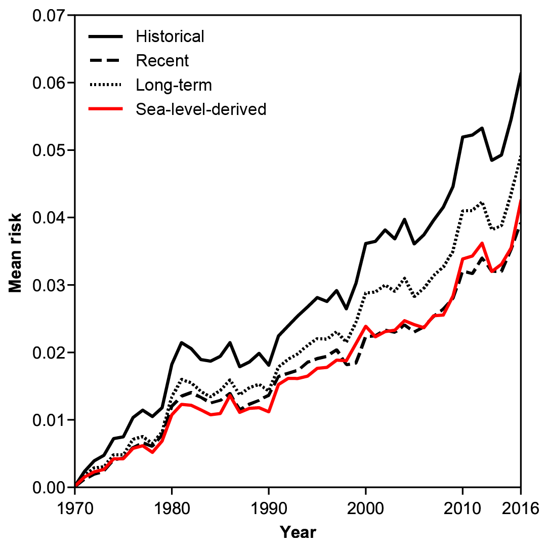
Figure 5Comparative evolution of mean risk over time under different representations of shoreline-change rate (hazard condition): historical (solid black), recent (dashed black), long term (dotted black), and derived from sea level (red).
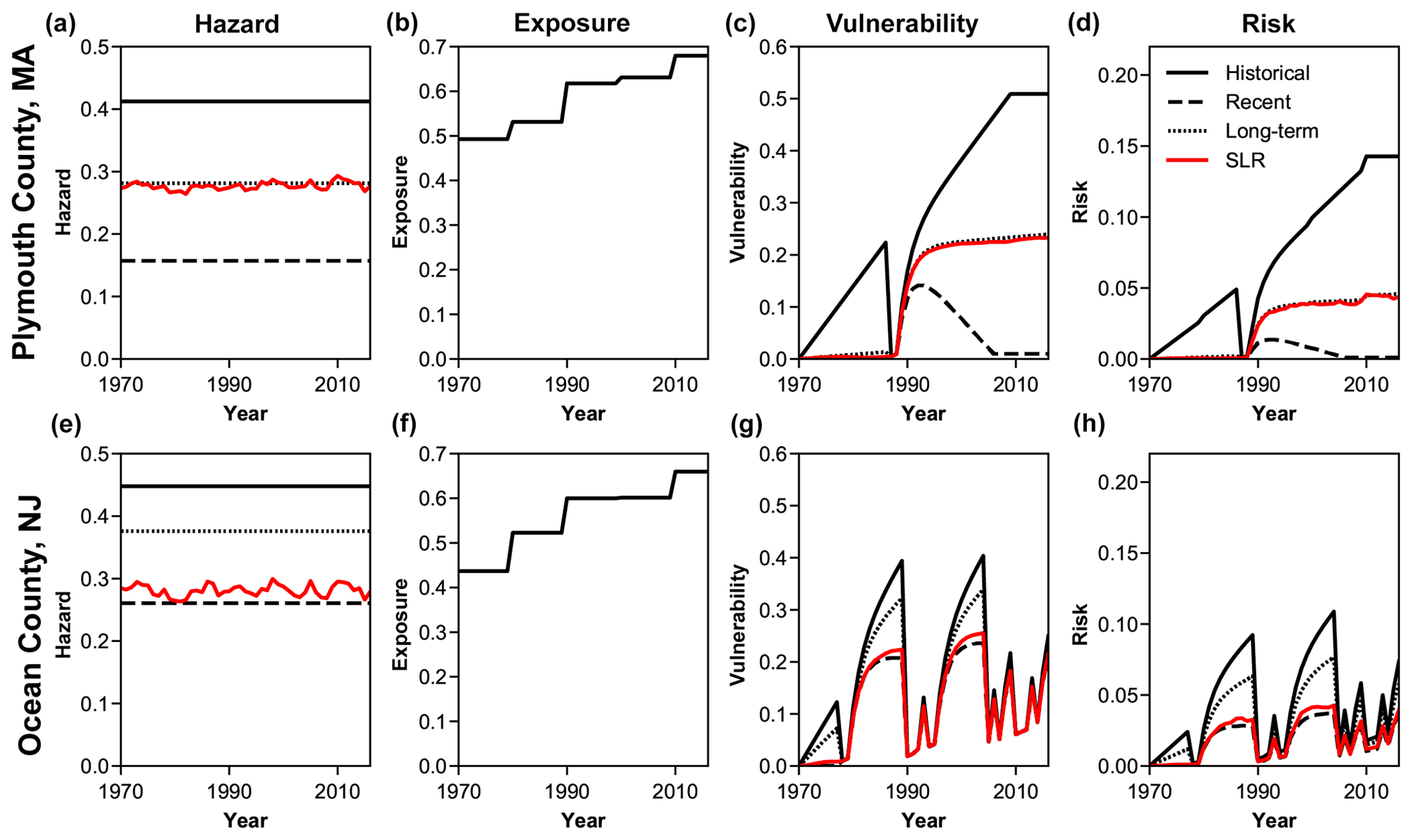
Figure 6Evolution of (a–c) mean components and (d) risk for Plymouth County, Massachusetts, and (e–h) Ocean County, New Jersey. Line type indicates results under a given hazard condition. Note that the vulnerability time series for Ocean County (g) shows the “ratchet effect” of cumulative vulnerability from repeated beach-nourishment episodes.
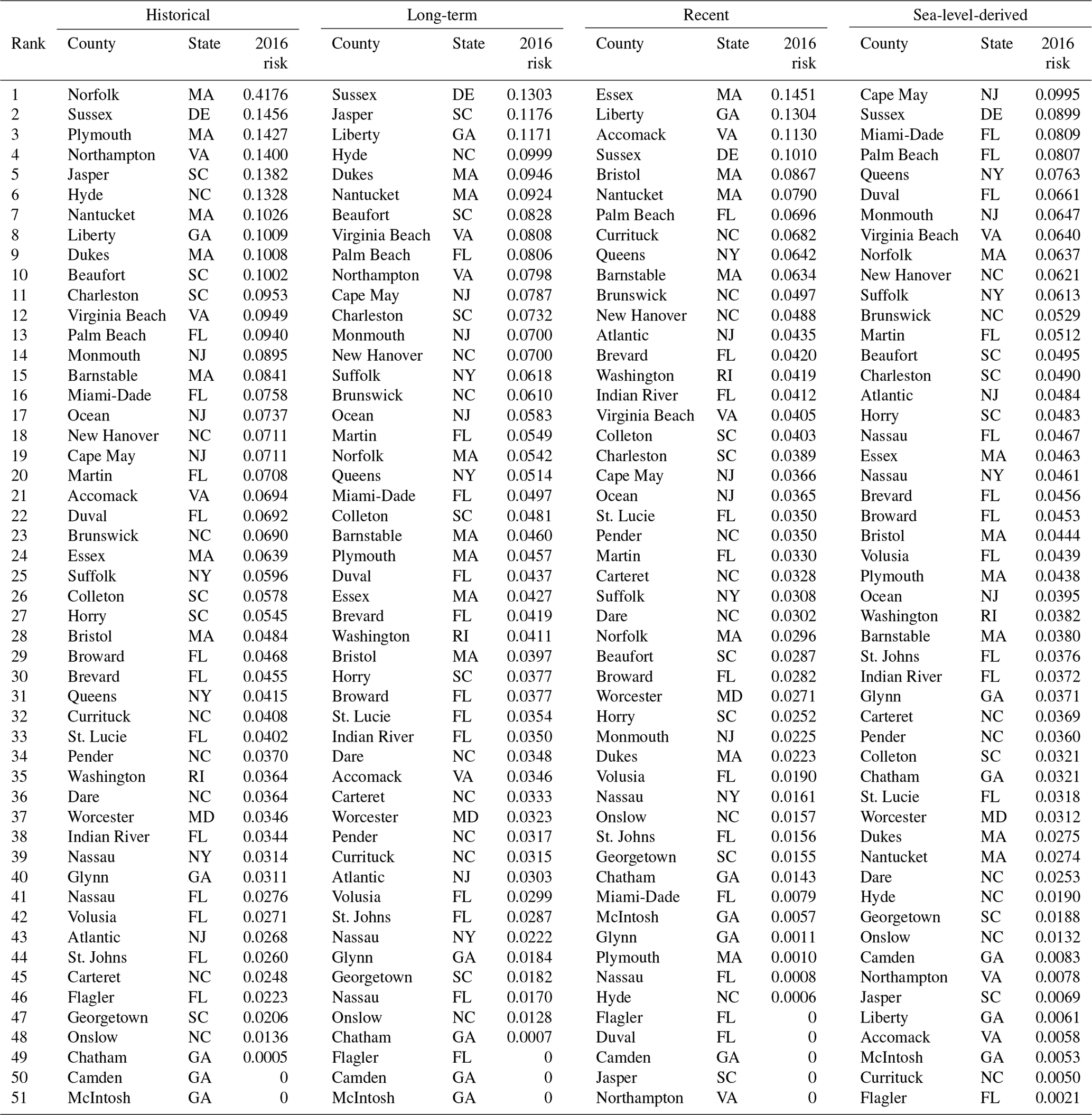
Individually, not all counties register rising risk trajectories over time. To compare how individual counties contribute to mean risk, we ranked each county by its risk index in 2016 (Table 1). We also examined in detail two examples of how individual counties responded to different hazards and beach-nourishment cycles (Fig. 6). Plymouth County, Massachusetts, demonstrates how vulnerability may respond to linear erosion rates (γ) that vary from eroding (negative, under the historical condition), to static (under the long-term and sea-level-derived conditions), to accreting (positive, under the recent condition) (Fig. 6a–d). Ocean County, New Jersey, demonstrates how the cumulative beach-nourishment factor (Vbn) can drive up risk (Fig. 6e–h). There, Vbn causes the local maxima and minima in vulnerability to increase over time (Fig. 6g), such that even when beaches are at full width, exposed property is still subject to vulnerability V>0. Ocean County highlights how the cumulative beach-nourishment factor functions as a ratchet that forces vulnerability to only increase over time. Because not every county practices beach nourishment, it is possible for a county to have V=0 if its shoreline is accreting (e.g. Camden and McIntosh counties, Georgia). A county that never nourishes will have a Vbn=0, and if a county nourishes only once or twice then their Vbn will remain negligible (but not negative). However, mean vulnerability is greater – and therefore mean risk is greater – when Vbn is left out (V=Vbw) (Fig. S1c and d) because its inclusion makes vulnerability less sensitive to changes in beach width. For example, a county that does not nourish could have a narrow beach but a low Vbn and therefore a lower vulnerability score than if its vulnerability were only a function of beach width.
Table 1Counties ranked by risk in 2016, calculated with historic, long-term, recent, and sea-level-derived shoreline-change rates.
Alongshore mean risk in our model also increases because of a well-documented national trend in exposure (NOAA, 2013). Exposure in an individual county may increase or decrease from one decade to the next, but mean exposure along the full span of the coast increases over time (NOAA, 2013; Union of Concerned Scientists, 2018). The 51 coastal counties in this analysis represent 1.6 % of all US counties, but since 1970 have constituted 6.9 %–9.25 % of the total value of all owner-occupied housing units in the country (Fig. S2). Thus, while our data-driven model includes simplifying assumptions, we suggest that the increasing risk trends in our findings represent a real phenomenon since exposure has risen at the coast decade for decade in real terms, and our cumulative beach-nourishment factor both dampens mean vulnerability and highlights the reality of long-term risk in counties that nourish continually.
3.2 Component relationships
Finally, we compared the statistical distributions of exposure in high- and low-hazard counties and in high- and low-intensity-nourishing counties (as an aspect of vulnerability), to examine whether the three components of risk, as we represent them, reflect temporal interrelationships. In keeping with the scaled stripes in Figs. 1, 2, and 4, we present these distributions (Figs. 7 and 8) at the transect scale rather than the county scale to better represent the contributions of counties by their coastal extents. For example, Queens County, NY, hosts a high density of exposure per alongshore kilometre – very high exposure and a short coastline – and contributes only four transects to the total (Fig. 2). Likewise, because of its size, Dare County, NC, has both high exposure and a longer shoreline, resulting in a lower value of exposure per alongshore kilometre that accounts for over 100 transects of the domain. Overall, Dare County is less densely developed than Queens County. However, our treatment of exposure does overlook concentrated areas of high-density development within otherwise low-density counties – hotspots at which hazard, exposure, and vulnerability (i.e. nourishment activity) may be closely related.
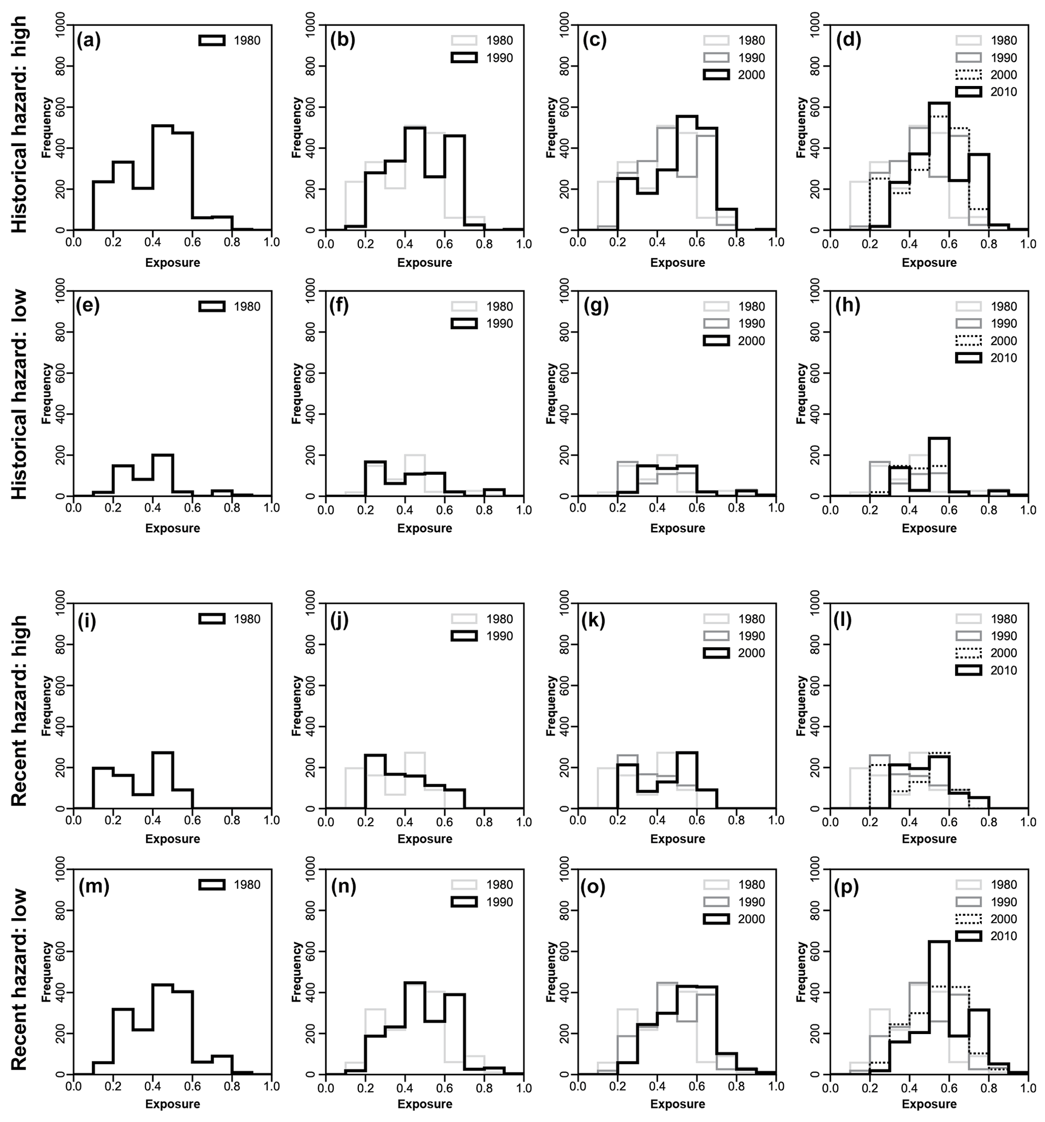
Figure 7Transect-level distribution of exposure per coastal kilometre, by decade, under (a–h) high and low historical and (i–p) high and low recent shoreline-change hazard. “High” hazard here is a value greater than 0.272 (the normalized value for a shoreline-change rate of zero); “low” hazard is a value greater than 0.272. High hazard therefore indicates erosion, and low hazard indicates accretion. Summary statistics for these distributions are provided in Table S5.
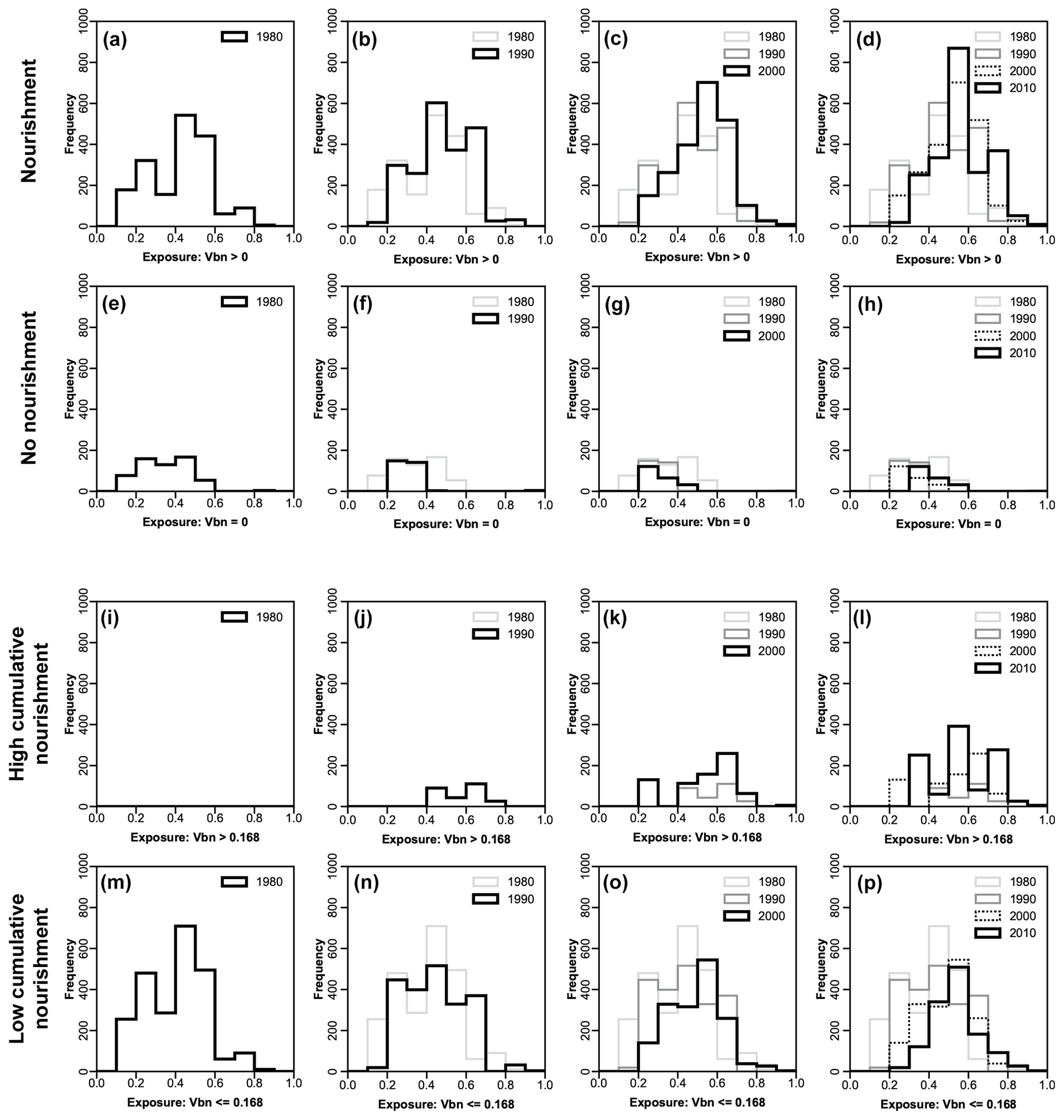
Figure 8Transect-level distribution of exposure per coastal kilometre, by decade, (a–h) in counties that have and have not nourished, and (i–p) in counties that have nourished above and below the 2016 median cumulative beach-nourishment index (Vbn=0.168). The 2016 median Vbn denotes the normalized value of the overall median cumulative number of nourishments across the domain. Summary statistics for these distributions are provided in Table S5.
To explore potential relationships between exposure and hazard, we sorted the exposure time series (Fig. 2) into counties associated with “high hazard” (eroding shorelines) and “low hazard” (accreting shorelines) for historical and recent shoreline change (Figs. 7 and S3). We find that exposure increases each decade in zones of high and low hazard alike, for both historical and recent shoreline change. Under historical shoreline-change hazard, exposure of property value is greatest in zones of high hazard (Figs. 7a–h and S3a). Conversely, exposure to high hazard is relatively low for recent shoreline-change rates (Figs. 7i–p and S3d), in part because recent shoreline-change rates tend to be less erosional than their historical counterparts (Fig. 3a). The difference between relative distributions of exposure in high and low hazard zones for historical shoreline-change rates increases in significance decade for decade, with a decreasing Kolmogorov–Smirnov p value that reflects the significance of their divergence (Fig. S3c). There is no such temporal divergence of exposure in high and low hazard zones for recent shoreline-change rates (Fig. S3f).
To explore, in parallel, potential relationships between exposure and vulnerability, we sorted the exposure time series into nourishing and non-nourishing counties and then by the intensity of beach nourishment (high or low) according to whether counties fell above or below the 2016 median value of cumulative Vbn (Figs. 8 and S4). We find that although exposure increases each decade in nourishing and non-nourishing counties alike, more property is ultimately exposed in nourishing counties. Moreover, the mean value of that exposed property increases at a greater rate than in non-nourishing counties (Figs. 8a–h and S4a–c). Initially, all property is exposed in counties where nourishment intensity is present but low (their Vbn sits below the 2016 median) – which we expect because for counties to accrue enough nourishment events to match the 2016 median cumulative-nourishment factor requires time (Fig. 8i and m). Exposure in intensively nourished counties (counties that accrue enough nourishment projects to have Vbn above the 2016 median) shows a marked increase in the 1980s (Fig. S4d). Total exposure in intensively nourished counties overtakes total exposure in sparsely nourished counties by the 2010s (Fig. S4e), such that more property ends up exposed in counties where nourishment intensity is high (Figs. 8i–p and S4d–f).
Both of these temporal relationships in spatial patterns of exposure and hazard (Fig. 7) and exposure and vulnerability (Fig. 8) are likely two vantages of the same feedback, catalysed by beach nourishment. Higher property value is exposed where historical shoreline-change hazard was high (Fig. 7a–d) and recent shoreline-change hazard is low (Fig. 7m–p) because those places also practice relatively intensive use of beach nourishment (Fig. 9). The cumulative effect of beach nourishment may be sufficiently strong to mask “true” rates of shoreline change (Armstrong and Lazarus, 2019) – a defensive intervention that, by reducing apparent hazard, may spur further development (Fig. 8), increasing exposure and creating demand for additional protection (Armstrong et al., 2016).
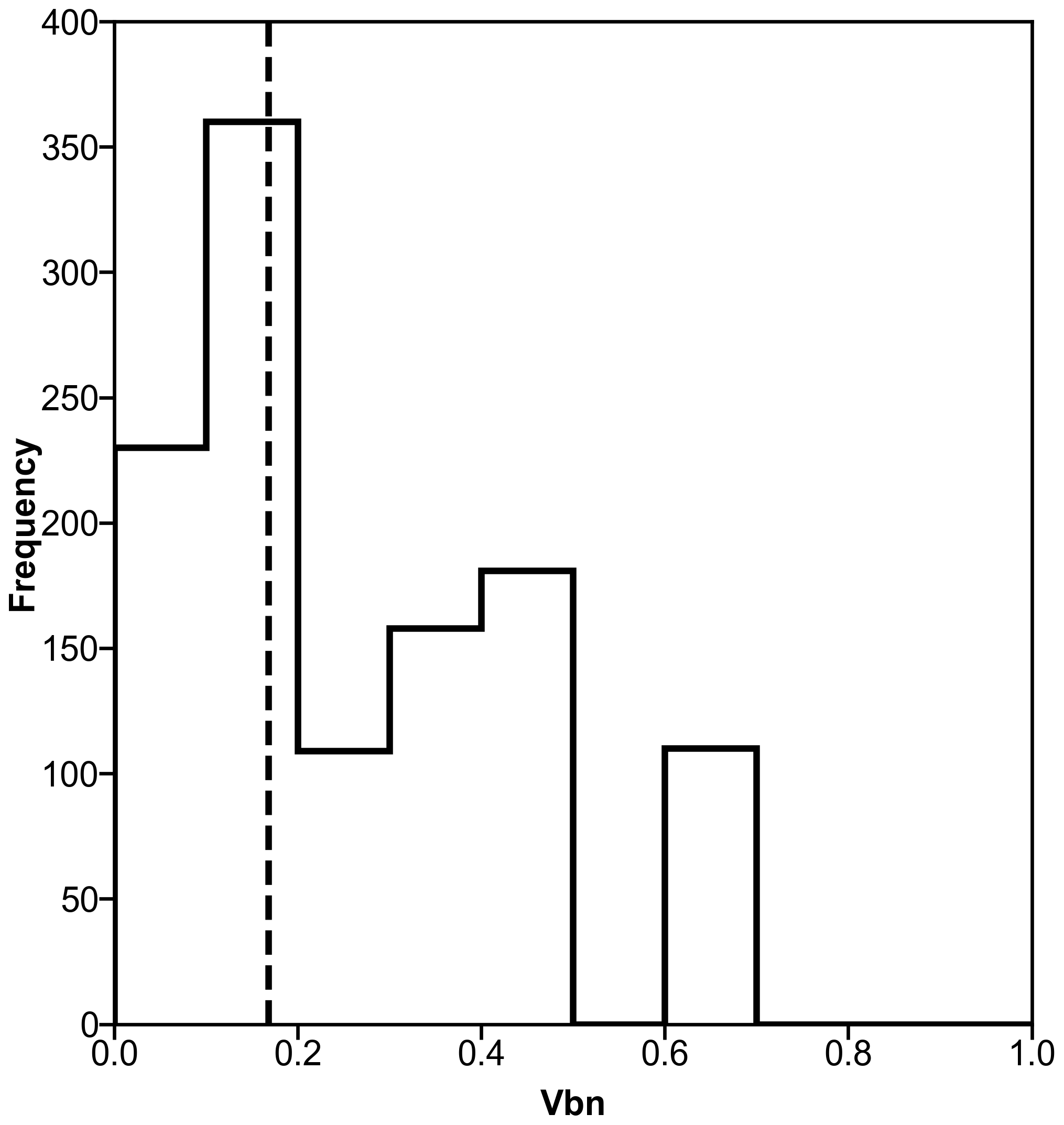
Figure 9Cumulative beach-nourishment index (Vbn), as of 2016, at transects (across all counties) that express both high “historical” and low “recent” rates of shoreline erosion (see Fig. 7a–d and m–p). The dotted line indicates the overall median Vbn=0.168 in 2016 for the full domain. For this component distribution, median Vbn=0.178 (mean = 0.251). This spatial correspondence between a major reversal in shoreline-change trend (from erosion to accretion) and above-average nourishment intensity is an indication of a coupling between chronic erosion (hazard) and defensive intervention (vulnerability).
Our data-driven, spatio-temporal model of risk along the US Atlantic coast produces trajectories that vary in space and, on average, rise over time for all four chronic hazard scenarios that we test (Fig. 5). We know from the underlying data that real exposure increases over time, but we suggest that our modelled risk trajectories also reflect intrinsic feedbacks between hazard, exposure, and vulnerability (Mileti, 1999). We find higher property exposure in counties with high-hazard historical shoreline-change rates and low-hazard recent shoreline-change rates (Fig. 7), and we find that exposure has increased more in places that have practised beach nourishment intensively (Fig. 8). The spatio-temporal relationships that we show between exposure and hazard (Fig. 7) and exposure and vulnerability (Fig. 8) may reflect a feedback between coastal development and beach nourishment (Fig. 9) (Armstrong et al., 2016; Armstrong and Lazarus, 2019) – a manifestation of the safe development paradox (Burby, 2006), in which hazard protections encourage further development in places prone to hazard impacts (Armstrong et al., 2016; Burby and French, 1981; Burby, 2006; Di Baldassarre et al., 2013, 2016; Keeler et al., 2018; Lazarus et al., 2016; McNamara and Lazarus, 2018; McNamara et al., 2015; Mileti, 1999; Smith et al., 2009; Werner and McNamara, 2007; White, 1945).
Our model is exploratory, and we reiterate its main caveats. Although there are many kinds of coastal hazard (e.g. storm impacts, flooding), we represented “chronic” hazard with shoreline-change rates that are spatially heterogeneous but temporally static. An alternative derivation of shoreline change, from sea-level rise rates and simplified shore slopes, varies in both space and time, and yielded overall results similar to those for the recent shoreline-change scenario. Exposure in our model only accounts for the monetary value of owner-occupied properties in coastal counties, as captured by the US census, thus excluding other potential measures of exposure, such as socio-economic indices (e.g. Cutter et al., 2006, 2008; Neumann et al., 2015; NRC, 2014; Samuels and Gouldby, 2005; Strauss et al., 2012), and requires that we spatially aggregate our analysis to county scales. Finally, our measure of vulnerability – intended to represent “susceptibility” (NRC, 2014; Samuels and Gouldby, 2005) without double-counting exposure or hazard – includes no method of shoreline protection other than beach nourishment and no explicit inclusion of storm recurrence or severity. Furthermore, our treatment of dynamic vulnerability is underpinned by a set of broad assumptions: that beaches comprise shorelines at the county scale, that in 1970 all counties have the same initial beach width, that a beach-nourishment project always restores a beach to its full width, and that counties with intensive nourishment programmes may render themselves more vulnerable over time by masking a chronic erosion problem (Armstrong and Lazarus, 2019; Pilkey and Cooper, 2014; Woodruff et al., 2018). We do not directly address alongshore spatial interactions within or between counties (Lazarus et al., 2011, 2016; Ells and Murray, 2012). Despite these assumptions, our model captures temporal interactions among the components of risk that ultimately yield large-scale spatial patterns similar to those identified in recent, fully empirical studies (Armstrong and Lazarus, 2019; Armstrong et al., 2016).
We suggest that models intended to test different coastal management policies, interventions, and scenarios should aim to include feedbacks between hazard, exposure, and vulnerability. In our data-driven model, traces of these feedbacks – and perhaps others – are likely embedded in the data we use. More detailed work at the intersection of theory and empiricism is necessary to resolve how feedbacks between hazard, exposure, and vulnerability dynamically affect each component of risk and to explore how different management interventions may mitigate – or exacerbate – the safe development paradox.
Datasets used in this work are publicly available: historical shorelines in the northeast (Himmelstoss et al., 2010; available: https://pubs.usgs.gov/of/2010/1119/, last access: November 2019) and southeast (Miller et al., 2005; available at https://pubs.usgs.gov/of/2005/1326/, last access: November 2019), coastal lidar (Doran et al., 2017; https://doi.org/10.5066/F7GF0S0Z), tide-gauge records (PSMSL, 2018: available at http://www.psmsl.org/data/obtaining/, last access: November 2019), historical census data (Minnesota Population Center, 2011; available at http://www.nhgis.org, last access: November 2019), and beach nourishment (PSDS, 2017; available at http://www.wcu.edu/1038.asp, last access: November 2019).
The supplement related to this article is available online at: https://doi.org/10.5194/nhess-19-2497-2019-supplement.
SBA and EDL conceived of the research; SBA performed the analysis; SBA and EDL collaborated on interpretation of the results; SBA led the writing of the paper, with contributions from EDL.
The authors declare that they have no conflict of interest.
This article is part of the special issue “Advances in computational modelling of natural hazards and geohazards”. It is a result of the Geoprocesses, Geohazards meeting – CSDMS 2018, Boulder, USA, 22–24 May 2018.
The authors thank Evan Goldstein, Julian Leyland, and James Dyke for helpful discussions.
This research has been supported by the Natural Environment Research Council (grant no. NE/N015665/2).
This paper was edited by Albert J. Kettner and reviewed by Jorge Lorenzo-Trueba and one anonymous referee.
AIR Worldwide: The Coastline at Risk: 2016 Update to the Estimated Insured Value, available at: http://airww.co/coastlineatrisk (last access: November 2019), 2016.
Arkema, K. K., Guannel, G., Verutes, G., Wood, S. A., Guerry, A., Ruckelshaus, M., Kareiva, P., Lacayo, M., and Silver, J. M.: Coastal habitats shield people and property from sea-level rise and storms, Nat. Clim. Change, 3, 913–918, https://doi.org/10.1038/nclimate1944, 2013.
Armstrong, S. B., Lazarus, E. D., Limber, P. W., Goldstein, E. B., Thorpe, C. and Ballinger, R. C.: Indications of a positive feedback between coastal development and beach nourishment, Earth's Future, 4, 626–635, https://doi.org/10.1002/2016EF000425, 2016.
Armstrong, S. B. and Lazarus, E. D.: Masked shoreline erosion at large spatial scales as a collective effect of beach nourishment, Earth's Future, 7, 74–84, https://doi.org/10.1029/2018EF001070, 2019.
Barbier, E. B., Hacker, S. D., Kennedy, C., Koch, E. W., Stier, A. C., and Silliman, B. R.: The value of estuarine and coastal ecosystem services, Ecol. Monogr., 81, 169–193, https://doi.org/10.1890/10-1510.1, 2011.
Blake, E. S., Landsea, C. W., and Gibney, E. J.: The deadliest, costliest, and most intense United States tropical cyclones from 1851 to 2010 (and other frequently requested Hurricane Facts), NOAA Tech. Memo. NWS NHC-6, NOAA, Miami, Florida, 2011.
Brown, S., Nicholls, R. J., Lowe, J. A., and Hinkel, J.: Spatial variations of sea-level rise and impacts: An application of DIVA, Climatic Change, 134, 403–416, https://doi.org/10.1007/s10584-013-0925-y, 2016.
Burby, R. J.: Hurricane Katrina and the paradoxes of government disaster policy: Bringing about wise governmental decisions for hazardous areas, Ann. Am. Acad. Pol. Soc. Sci., 604, 171–191, https://doi.org/10.1177/0002716205284676, 2006.
Burby, R. J. and French, S. P.: Coping with floods: the land use management paradox, J. Am. Plan. Assoc., 47, 289–300, https://doi.org/10.1080/01944368108976511, 1981.
Cooper, J. A. G. and Pilkey, O. H.: Sea-level rise and shoreline retreat: Time to abandon the Bruun Rule, Global Planet. Change, 43, 157–171, https://doi.org/10.1016/j.gloplacha.2004.07.001, 2004.
Cutter, S. L. and Emrich, C. T.: Moral hazard, social catastrophe: The changing face of vulnerability along the hurricane coasts, Ann. Am. Acad. Pol. Soc. Sci., 604, 102–112, https://doi.org/10.1177/0002716205285515, 2006.
Cutter, S. L. and Finch, C.: Temporal and spatial changes in social vulnerability to natural hazards, P. Natl. Acad. Sci. USA, 105, 2301–2306, https://doi.org/10.1073/pnas.0710375105, 2008.
Cutter, S. L., Emrich, C. T., Mitchell, J. T., Boruff, B. J., Gall, M., Schmidtlein, M. C., Burton, C. G., and Melton, G.: The long road home: Race, class, and recovery from Hurricane Katrina, Environment, 48, 8–20, https://doi.org/10.3200/ENVT.48.2.8-20, 2006.
Cutter, S. L., Barnes, L., Berry, M., Burton, C., Evans, E., Tate, E., and Webb, J.: A place-based model for understanding community resilience to natural disasters, Global Environ. Change, 18, 598–606, https://doi.org/10.1016/j.gloenvcha.2008.07.013, 2008.
Dean, R. G. and Dalrymple, R. A.: Coastal Processes with Engineering Applications, Cambridge University Press, Cambridge, 2001.
Desilver, D.: As American homes get bigger, energy efficiency gains are wiped out, Pew Res. Cent., available at: http://www.pewresearch.org/fact-tank/2015/11/09/as-american-homes-get-bigger-energy-efficiency-gains-are (last access: November 2019), 2015.
Di Baldassarre, G., Viglione, A., Carr, G., Kuil, L., Salinas, J. L., and Blöschl, G.: Socio-hydrology: Conceptualising human–flood interactions, Hydrol. Earth Syst. Sci., 17, 3295–3303, https://doi.org/10.5194/hess-17-3295-2013, 2013.
Di Baldassarre, G., Brandimarte, L. ,and Beven, K.: The seventh facet of uncertainty: wrong assumptions, unknowns and surprises in the dynamics of human–water systems, Hydrolog. Sci. J., 61, 1748–1758, https://doi.org/10.1080/02626667.2015.1091460, 2016.
Doran, K. S., Long, J. W., Birchler, J. J., Brenner, O. T., Hardy, M. W., Morgan, K. L. M., Stockdon, H. F., and Torres, M. L.: Lidar-derived beach morphology (dune crest, dune toe, and shoreline) for U.S. sandy coastlines (ver. 2.0 August 2018): US Geological Survey data release, Lidar-derived beach Morphol. (dune crest, dune toe, shoreline) US sandy coastlines, US Geol. Surv. data release, https://doi.org/10.5066/F7GF0S0Z, 2017.
Ells, K. and Murray, A. B.: Long-term, non-local coastline responses to local shoreline stabilization, Geophys. Res. Lett. 39, L19401, https://doi.org/10.1029/2012GL052627, 2012.
Estrada, F., Botzen, W. J. W., and Tol, R. S. J.: Economic losses from US hurricanes consistent with an influence from climate change, Nat. Geosci., 8, 880–885, https://doi.org/10.1038/NGEO2560, 2015.
Hapke, C. J., Kratzmann, M. G., and Himmelstoss, E. A.: Geomorphic and human influence on large-scale coastal change, Geomorphology, 199, 160–170, https://doi.org/10.1016/j.geomorph.2012.11.025, 2013.
Himmelstoss, E. A., Kratzmann, M., Hapke, C., Thieler, E. R., and List, J.: USGS Open-File Report 2010-1119: National Assessment of Shoreline Change: A GIS Compilation of Vector Shorelines and Associated Shoreline Change Data for the New England and Mid-Atlantic Coasts, available at: https://pubs.usgs.gov/of/2010/1119/ (last access: November 2019), 2010.
Hinkel, J., Nicholls, R. J., Vafeidis, A. T., Tol, R. S. J., and Avagianou, T.: Assessing risk of and adaptation to sea-level rise in the European Union: An application of DIVA, Mitig. Adapt. Strateg. Glob. Change, 15, 703–719, https://doi.org/10.1007/s11027-010-9237-y, 2010.
Holgate, S. J., Matthews, A., Woodworth, P. L., Rickards, L. J., Tamisiea, M. E., Bradshaw, E., Foden, P. R., Gordon, K. M., Jevrejeva, S., and Pugh, J.: New data systems and poducts at the Permanent Service for Mean Sea Level, J. Coast. Res., 288, 493–504, https://doi.org/10.2112/JCOASTRES-D-12-00175.1, 2013.
Johnson, J. M., Moore, L. J., Ells, K., Murray, A. B., Adams, P. N., MacKenzie, R. A., and Jaeger, J. M.: Recent shifts in coastline change and shoreline stabilization linked to storm climate change, Earth Surf. Proc. Land., 40, 569–585, https://doi.org/10.1002/esp.3650, 2015.
Keeler, A. G., Mcnamara, D. E., and Irish, J. L.: Responding to Sea Level Rise: Does short-term risk reduction inhibit successful long-term adaptation?, Earth's Future, 6, 1–4, https://doi.org/10.1002/2018EF000828, 2018.
Lazarus, E. D., McNamara, D. E., Smith, M. D., Gopalakrishnan, S., and Murray, A. B.: Emergent behavior in a coupled economic and coastline model for beach nourishment, Nonlin. Process. Geophys., 18, 989–999, https://doi.org/10.5194/npg-18-989-2011, 2011.
Lazarus, E. D., Ellis, M. A., Brad Murray, A., and Hall, D. M.: An evolving research agenda for human-coastal systems, Geomorphology, 256, 81–90, https://doi.org/10.1016/j.geomorph.2015.07.043, 2016.
Lentz, E. E., Thieler, E. R., Plant, N. G., Stippa, S. R., Horton, R. M., and Gesch, D. B.: Evaluation of dynamic coastal response to sea-level rise modifies inundation likelihood, Nat. Clim. Change, 6, 696–700, https://doi.org/10.1038/nclimate2957, 2016.
Lorenzo-Trueba, J. and Ashton, A. D.: Rollover, drowning, and discontinuous retreat: Distinct modes of barrier response to sea-level rise arising from a simple morphodynamic model, J. Geophys. Res.-Ea. Surf., 119, 779–801, https://doi.org/10.1002/2013JF002941, 2014.
McNamara, D. E. and Lazarus, E. D.: Barrier Islands as Coupled Human-Landscape Systems, in: Barrier Dynamics and Response to Changing Climate, edited by: Moore, L. J. and Murray, A. B., Springer International Publishing, London, 363–383, 2018.
McNamara, D. E., Gopalakrishnan, S., Smith, M. D., and Murray, A. B.: Climate adaptation and policy-induced inflation of coastal property value, PLoS One, 10, e0121278, https://doi.org/10.1371/journal.pone.0121278, 2015.
Mileti, D.: Disasters by Design: A Reassessment of Natural Hazards in the United States, Joseph Henry Press, Washington, D.C.,, 1999.
Miller, T. L., Morton, R. A., and Sallenger, A. H.: USGS Open File Report 2005-1326: The National Assessment of Shoreline Change: A GIS Compilation of Vector Shorelines and Associated Shoreline Change Data for the US Southeast Atlantic Coast, available at: https://pubs.usgs.gov/of/2005/1326/ (last access: Novmeber 2019), 2005.
Minnesota Population Center: National Historical Geographic Information System: Version 2.0., available at: http://www.nhgis.org (last access: November 2019), 2011.
Neumann, B., Vafeidis, A. T., Zimmermann, J., and Nicholls, R. J.: Future coastal population growth and exposure to sea-level rise and coastal flooding: A global assessment, PLoS One, 10, e0118571, https://doi.org/10.1371/journal.pone.0118571, 2015.
Nicholls, R. J. and Cazenave, A.: Sea-level rise and its impact on coastal zones, Science, 328, 1517–1520, https://doi.org/10.1126/science.1185782, 2010.
NOAA – National Oceanic and Atmospheric Administration: National Coastal Population Report, available at: https://coast.noaa.gov/digitalcoast/training/population-report.html (last access: November 2019), 2013.
NRC – National Research Council: Beach Nourishment and Protection, National Acadamy Press, Washington, D.C., 1995.
NRC – National Research Council: Reducing Coastal Risks on the East and Gulf Coasts, National Acadamy Press, Washington, D.C., 2014.
Parris, A., Bromirski, P., Burkett, V., Cayan, D., Culver, M., Hall, J., Horton, R., Knuuti, K., Moss, R., Obeysekera, J., Sallenger, A., and Weiss, J.: Global Sea Level Rise Scenarios for the US National Climate Assessment, NOAA Tech Memo OAR CPO, 1–37, available at: http://cpo.noaa.gov/sites/cpo/Reports/2012/NOAA_SLR_r3.pdf (last access: November 2019), 2012.
Pielke Jr., R. A., Gratz, J., Landsea, C. W., Collins, D., Saunders, M. A., and Musulin, R.: Normalized hurricane damage in the United States: 1900–2005, Nat. Hazards Rev., 9, 29–42, https://doi.org/10.1061/(ASCE)1527-6988(2008)9:1(29), 2008.
Pilkey, O. H. and Cooper, J. A. G.: Are natural beaches facing extinction?, J. Coast. Res., 70, 431–436, https://doi.org/10.2112/SI70-073.1, 2014.
PSDS – Program for the Study of Developed Shorelines: PSDS: Beach nourishment database, Program for the Study of Developed Shorelines, available at: http://www.wcu.edu/1038.asp (last access: November 2019), 2017.
PSMSL – Permanent Service for Mean Sea Level: Tide Gauge Data, available at: http://www.psmsl.org/data/obtaining/, last access: 17 September 2018.
Sallenger, A. H., Doran, K. S., and Howd, P. A.: Hotspot of accelerated sea-level rise on the Atlantic coast of North America, Nat. Clim. Change, 2, 884–888, https://doi.org/10.1038/nclimate1597, 2012.
Samuels, P. and Gouldby, B.: Language of Risk: Project Definitions, Floodsite: Integrated flood risk analysis and management methodologies, Report T32-04-01, available at: http://www.floodsite.net/html/partner_area/project_docs/floodsite_language_of_risk_v4_0_p1.pdf (last access: November 2019), 2005.
Smallegan, S. M., Irish, J. L., Van Dongeren, A. R., and Den Bieman, J. P.: Morphological response of a sandy barrier island with a buried seawall during Hurricane Sandy, Coast. Eng., 110, 102–110, https://doi.org/10.1016/j.coastaleng.2016.01.005, 2016.
Smith, M. D., Slott, J. M., McNamara, D., and Murray, A. B.: Beach nourishment as a dynamic capital accumulation problem, J. Environ. Econ. Manage., 58, 58–71, https://doi.org/10.1016/j.jeem.2008.07.011, 2009.
Strauss, B. H., Ziemlinski, R., Weiss, J. L., and Overpeck, J. T.: Tidally adjusted estimates of topographic vulnerability to sea level rise and flooding for the contiguous United States, Environ. Res. Lett., 7, 014033, https://doi.org/10.1088/1748-9326/7/1/014033, 2012.
Taylor, N. R., Irish, J. L., Udoh, I. E., Bilskie, M. V., and Hagen, S. C.: Development and uncertainty quantification of hurricane surge response functions for hazard assessment in coastal bays, Nat. Hazards, 77, 1103–1123, https://doi.org/10.1007/s11069-015-1646-5, 2015.
Temmerman, S., Meire, P., Bouma, T. J., Herman, P. M. J., Ysebaert, T., and De Vriend, H. J.: Ecosystem-based coastal defence in the face of global change, Nature, 504, 79–83, https://doi.org/10.1038/nature12859, 2013.
Thieler, E. R., Himmelstoss, E. A., Zichichi, J. L., and Ergul, A.: Digital Shoreline Analysis System (DSAS) version 4.0: An ArcGIS extension for calculating shoreline change, in: US Geological Survey Open-File Report 2008-1278, Reston, Virginia, available at: https://woodshole.er.usgs.gov/project-pages/DSAS/version4/ (last access: November 2019), 2008.
Union of Concerned Scientists: Underwater: Rising Seas, Chronic Floods, and the Implications for US Coastal Real Estate, available at: https://www.ucsusa.org/sites/default/files/attach/2018/06/underwater-analysis-full-report.pdf (last access: November 2019), 2018.
UNISDR – United Nations Office for Disaster Risk Reduction: Sendai Framework for Disaster Risk Reduction 2015–2030, available at: https://www.unisdr.org/we/coordinate/sendai-framework (last access: November 2019), 2015.
Werner, B. T. and McNamara, D. E.: Dynamics of coupled human-landscape systems, Geomorphology, 91, 393–407, https://doi.org/10.1016/j.geomorph.2007.04.020, 2007.
White, G. F.: Human adjustments to floods, Department of Geography Research, Paper no. 29, University of Chicago, Chicago, 1945.
Witze, A.: Attack of the extreme floods, Nature, 555, 156–158, https://doi.org/10.1038/d41586-018-02745-0, 2018.
Wolinsky, M. A. and Murray, A. B.: A unifying framework for shoreline migration: 2. Application to wave-dominated coasts, J. Geophys. Res.-Ea. Surf., 114, F01009, https://doi.org/10.1029/2007JF000856, 2009.
Wong, P. P., Losada, I. J., Gattuso, J.-P., Hinkel, J., Khattabi, A., McInnes, K. L., Saito, Y., and Sallenger, A.: Coastal systems and low-lying areas, in: Climate Change 2014: Impacts, Adaption, and Vulnerability. Part A: Global and Sectoral Aspects, Contribution of Working Group II to the Fifth Assessment Report of the Intergovernmental Panel on Climate Change, edited by: Field, C. B., Barros, V. R., Dokken, D. J., Mach, K. J., Mastrandrea, M. D., Bilir, T. E., Chatterjee, M., Ebi, K. L., Estrada, Y. O., Genova, R. C., Girma, B., Kissel, E. S., Levy, A. N., MacCracken, S., Mastrandrea, P. R., and White, L. L., Cambridge University Press, Cambridge, UK and New York, NY, USA, 361–409, 2014.
Woodruff, S., BenDor, T. K., and Strong, A. L.: Fighting the inevitable: infrastructure investment and coastal community adaptation to sea level rise, Syst. Dyn. Rev., 34, 48–77, https://doi.org/10.1002/sdr.1597, 2018.