the Creative Commons Attribution 4.0 License.
the Creative Commons Attribution 4.0 License.
 | 04 Dec 2019
Three-dimensional rockfall shape back analysis: methods and implications
David A. Bonneau
D. Jean Hutchinson
Paul-Mark DiFrancesco
Melanie Coombs
Zac Sala
Rockfall is a complex natural process that can present risks to the effective operation of infrastructure in mountainous terrain. Remote sensing tools and techniques are rapidly becoming the state of the practice in the characterization, monitoring and management of these geohazards. The aim of this study is to address the methods and implications of how the dimensions of three-dimensional rockfall objects, derived from sequential terrestrial laser scans (TLSs), are measured. Previous approaches are reviewed, and two new methods are introduced in an attempt to standardize the process. The approaches are applied to a set of synthetic rockfall objects generated in the open-source software package Blender. Fifty rockfall events derived from sequential TLS monitoring in the White Canyon, British Columbia, Canada, are used to demonstrate the application of the proposed algorithms. This study illustrates that the method used to calculate the rockfall dimensions has a significant impact on how the shape of a rockfall object is classified. This has implications for rockfall modelling as the block shape is known to influence rockfall runout.


In steep mountainous regions around the world, infrastructure such as highways and railways may be subject to rockfall hazards. A rockfall can be defined as discrete fragments of rock which have detached from a cliff and subsequently fall, bounce and roll as the fragments move downslope by gravity (Hungr et al., 2014). Rockfalls can triggered by several factors such as freeze–thaw cycles, weathering, heavy rainfall, root action, seismicity and others (Volkwein et al., 2011). High energy and mobility are also characteristics of rockfalls, making them a major cause of landslide fatalities (Guzzetti et al., 2004). Moreover, these geohazards can result in economic losses due to service interruptions and equipment damage.
To assist in the management of these geohazards, a rockfall hazard analysis can be undertaken to qualitatively or quantitatively define the rockfall hazard present along a section of linear infrastructure. A typical rockfall hazard analysis involves the compilation of known rockfall events over a specific spatial scale and within a set period of time (Volkwein et al., 2011). Inventories aim to provide a better understanding about the spatio-temporal occurrence and magnitude of events (Froude and Petley, 2018). Ultimately, temporal trends can be identified from an inventory, which supports a more systematic mapping of hazards in the region to help mitigate future losses. It may also be useful to discern any long-term changes that are projected, as extreme weather events are expected to increase in both frequency and magnitude within a changing climate (Cloutier et al., 2016).
Once an inventory has been assembled, power law distributions have been suggested to characterize the frequency–magnitude relationship for rockfall at the study slope (Hungr et al., 1999). Using the rockfall frequency–magnitude relationship at the study slope, characterized by specific geological and geomorphological features, return periods for select volume ranges can be determined (Wieczorek and Jäger, 1996; Hungr et al., 1999; Dussauge et al., 2003; Malamud et al., 2004).
Remote sensing techniques, such as terrestrial laser scanning (TLS), have been used to characterize and monitor rockfall hazards (Abellán et al., 2014; Jaboyedoff et al., 2012; Telling et al., 2017). Single epoch TLS scans can be used for structural characterization of discontinuity orientations (Lato et al., 2009), the determination of the size and spatial distribution of potentially unstable rock mass volumes (Sturzenegger et al., 2011), and the back calculation of rockfall volumes based on discontinuity orientations of identified rockfall scars (Santana et al., 2012). Work by Lato et al. (2012), demonstrates how TLS can be integrated into rockfall hazard assessments along road cuts. Rockfall magnitude, block size distribution and block shape distribution were measured using surface models derived from TLS scans. This information can be directly integrated into rockfall modelling for rockfall hazard evaluation.
With multi-temporal TLS datasets, change detection algorithms, such as M3C2 (Lague et al., 2013), as an example, can be used to identify areas of loss on slopes (i.e. rockfall) between sequential TLS scans. The location, volume and dimensions of rockfall on the slope can be calculated and populated into a database, as demonstrated by Rosser et al. (2007), Guerin et al. (2014), Tonini and Abellán (2014), van Veen et al. (2017), Janeras et al. (2017) and Williams et al. (2018). In several of these studies, smaller magnitude rockfalls have been identified, which are generally not observed during field inspections performed from the base of the slope. Furthermore, smaller rockfall events have been shown to bound the area of larger deforming portions of the slope (Kromer et al., 2015).
Recent work by Williams et al. (2018) makes use of a fully automated terrestrial laser scanning system to near-continuously monitor a section of coastal cliff in the United Kingdom. With near-real-time processing capabilities, they demonstrate the influence of temporal acquisition rate on the calculated frequency–magnitude relationship for rockfall at the study slope. They demonstrate that more frequent monitoring captures a higher proportion of smaller magnitude rockfall events, which represents a higher frequency magnitude scaling coefficient. However, due to the 2.5-D nature of the volumetric analysis, smaller magnitude events resulted in a higher degree of volumetric uncertainty, due to edge effects compounded when 3-D change maps are converted to 2.5-D raster datasets.
With the rapid automation of TLS acquisition and change detection processing workflows (Kromer et al., 2017; Williams et al., 2018), practitioners are able to evaluate potential rockfall events and their characteristics quickly and with substantial detail (Abellán et al., 2014). TLS systems are portable and can be deployed on a tripod as soon as the site is accessed. There is no need to establish a baseline dataset as is the case with radar systems, for example (Teza et al., 2008). In addition, TLS systems can achieve high spatial resolution of measurements (Pesci et al., 2011). These strengths of TLS systems facilitate detailed back analysis of rockfall events to assess characteristics which can then be used for ongoing rockfall hazard analysis. With the recent advances in rockfall modelling with rigid body physics, models can utilize the exact shape and position of the block detachment location (Harrap et al., 2019). These cases can be used for both calibration of the model and development of more representative hazard mapping. Preliminary studies of the rockfall runout with respect to rockfall shape have been conducted by Glover (2015) and Sala (2018). Both authors found that the shape of the rockfall object has a pronounced effect on runout behaviour. This behaviour has direct implications for rockfall hazard zoning. Therefore, the ability to characterize the shape of rockfall events is a key component which needs to be considered in generating rockfall databases from sequential TLS scans. A variety of different formulations have been proposed to measure the shape of rockfalls from point cloud datasets, which record the before and after failure geometry. The authors highlight several methods which have been used in other studies and present two new methodologies to determine the dimensions of a rockfall object.
1.1 Rockfall shape and dimensions
The quantification of the shape of a rockfall scar can provide insight into the kinematics of failure and potential runout of detached material fragments. The use of remote sensing techniques and 3-D change detection algorithms permits extraction of true rockfall shape, yet limited work has been completed to quantify shape, despite its pronounced effect on runout behaviour (Glover, 2015; Sala, 2018). Shape, as noted by Blott and Pye (2008), is a function of four primary characteristics which include form, roughness, irregularity and sphericity. Readers are referred to Blott and Pye (2008) for further details on these characteristics.

Figure 1Overview of the Sneed and Folk ternary diagram adapted from Blott and Pye (2008). (a) Visual representation of the different shape forms as defined by Sneed and Folk (1958). Inset diagrams display the divisions for each shape class. (b) Overview of the rounded synthetic blocks generated using Blender. (c) Overview of the angular blocks generated using Blender.
In 1958, Sneed and Folk (1958) introduced a ternary diagram (Fig. 1a) to describe the shape of pebbles based on relations between the long (A), intermediate (B) and short orthogonal axes (C). The three ratios are listed below.
Based on the three relations described above, particles can be classified into 10 different shape classes. The end members of the ternary diagram are compact (cubic), platy (tabular), and elongated (rod shaped).
In addition to granular particle shape classification, the Sneed and Folk ternary diagram has been used in rockfall studies to characterize rockfall dimensions and shape (Benjamin, 2018; van Veen et al., 2017; Williams, 2017). In the aforementioned studies, the rockfall dimensions were computed using a bounding box approach. A bounding box defines the minimum extents of a cuboid which fully encloses the set of points defining the object. In this study and the aforementioned studies, the bounding box is oriented such that the edges of the calculated box are parallel to Cartesian coordinate axes.
Currently there is no standardized method to determine the dimensions of a rockfall object extracted from remote sensing data, such that the rockfall shape can be classified. There is uncertainty in evaluating both the distance and orientation of the axis lengths. This uncertainty is compounded by the fact that there is ambiguity about whether the axis measurements are to be mutually orthogonal or not. In this work, the authors address these uncertainties and propose standardized methods to evaluate the dimensions of a rockfall object.
1.2 Objectives
In this work, the authors address the process of extracting information regarding rockfall dimensions from remotely sensed datasets. The primary objectives of this work are summarized below.
-
Review current approaches used to determine the dimensions of 3-D rockfall objects.
-
Present two new approaches for extracting the dimensions from 3-D rockfall objects represented by point clouds.
-
Apply all of the approaches to a dataset of synthetic 3-D rockfall objects.
-
Implement the proposed approaches on a rockfall database derived from terrestrial laser scanning (TLS) at the White Canyon in the Thompson River valley in Interior British Columbia, Canada (Fig. 2).
-
Determine which method(s) provide(s) the most accurate measurements of the objects' three mutually orthogonal principal axes.
A rockfall object in this context is defined as a three-dimensional (3-D) point cloud or mesh that approximates the geometry and volume of rock that detached from the slope.
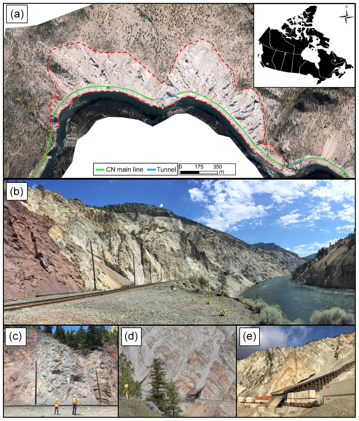
Figure 2Location map of the White Canyon. (a) October 2015 orthophoto of the White Canyon. The White Canyon is delineated by the red dashed line. (b) July 2016 panoramic photograph from track level looking northeast at the complex morphology of the study slope. (c) July 2016 photograph from track level of the Mt. Lytton batholith. (d) April 2017 photograph displaying the TLS system setup looking at the study slope from across the Thompson River. (e) February 2018 photograph from track level looking at one of the rock sheds on the eastern portion of the canyon. The rock shed is 20 m in width.
The methodology involves applying six different approaches to measure the geometry of irregularly shaped blocks and evaluating the output using the range of shapes described in the Sneed and Folk ternary diagram (Sect. 2.1). Both synthetically generated (Sect. 2.1) and real rock shapes were assessed. The methods by which data were collected and processed for the real rock shapes using both terrestrial laser scanning (TLS) and structure-from-motion multi-view-stereo (SfM-MVS) photogrammetry are discussed in Sect. 2.2. Section 2.3 presents the methodology used to extract rockfall information from 3-D change detection. Section 2.4 describes the six approaches used to extract dimension information from 3-D point clouds of rockfall shapes.
2.1 Synthetic block dataset
A synthetic block dataset was generated in the open-source software package Blender (Blender, 2018) using the process described by Sala (2018) to generate synthetic blocks for rockfall simulation. In general, the process involves the sculpting of cubic meshes that encompass 1 m3 of volume. Mesh sculpting in Blender allows for the displacement of mesh geometries into a variety of different shapes, taking into consideration block form characteristics, such as angularity. Once a shape has been created, its mesh is subdivided, increasing the number of vertices on the shape's surface to better match the point density which can be achieved from the TLS data described in the following sections. The mesh vertices are then exported, creating a synthetic rockfall block point cloud. Blocks corresponding to each major class in the Sneed and Folk ternary diagram were created. For each class, (i.e. platy, elongate, cubic, etc.) a rounded and an angular version, as defined by Powers (1953), of the block was generated. Figure 1b displays examples of the blocks used in this study.
2.2 Remote sensing data acquisition
The following subsections (Sect. 2.2.1 and 2.2.2) outline the remote sensing techniques that are used in this study to collect point cloud data to define the geometry of real rockfalls.
2.2.1 Terrestrial laser scanning (TLS)
Terrestrial laser scans were taken with an Optech Ilris 3D-ER terrestrial laser scanner (Fig. 2d). The Optech Ilris has a manufacturer-specified accuracy of 7 mm in range and 8 mm in vertical and horizontal directions for data collected from a distance of 100 m (Optech, 2014). The maximum range for the Optech Ilris is approximately 800 m with 20 % target reflectivity (Pesci et al., 2011).
Due to the complex geometry of the rock slopes in the White Canyon, several overlapping scans from different vantage points were captured to minimize occlusions and to decrease the lateral incidence angle in the scans of the slope. Point spacing for each scan varied between 7 and 10 cm. The scan site locations are displayed in Fig. 3, along with a timeline of the scans used in the study. Scans were taken approximately every 2–3 months starting in November 2014. The last set of TLS scans used in the analysis were taken in December 2017.
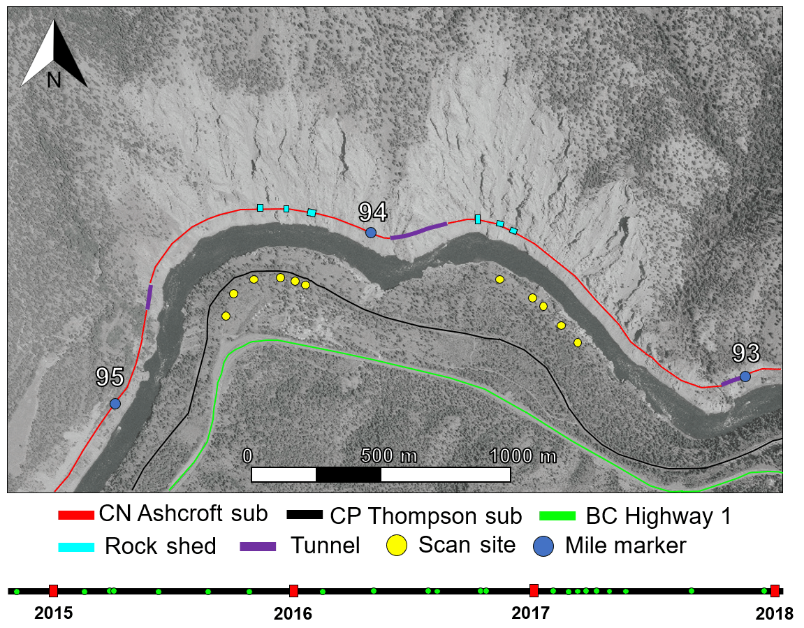
Figure 3Overview of the scan site locations from across the Thompson River. The timeline across the bottom of the figure indicates the times when TLS scans were captured (green dots).
To process the TLS scans, the scans were first parsed using Optech Parsing software. Once parsed, vegetation, mesh, and railway infrastructure components such as slide detector fences were manually removed from the raw point cloud using PolyWorks PIFEdit. After the point clouds were cleaned, they were aligned using PolyWorks ImAlign to a common baseline (November 2014). The alignment process consisted of a coarse alignment using point picking and then a fine alignment using an iterative closest point (ICP) algorithm (Besl and McKay, 1992). Areas of known change on the slope were excluded from the alignment process to help improve the alignment between sequential scans (Lato et al., 2015).
2.2.2 Structure-from-motion multi-view-stereo (SfM-MVS) photogrammetry
Structure-from-motion multi-view-stereo (SfM-MVS) photogrammetry models were generated of both White Canyon East (WCE) and White Canyon West (WCW) (Fig. 4). The Agisoft PhotoScan Professional V1.3.2 software package (Agisoft LLC, 2018) was used to create the models. The models were generated following a typical SfM-MVS photogrammetry processing workflow (Smith et al., 2016; Westoby et al., 2012).
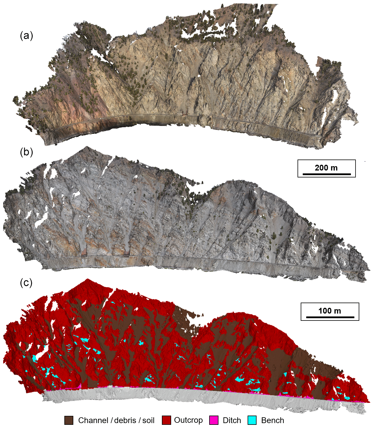
Figure 4Overview of the SfM-MVS photogrammetry models. (a) Model of White Canyon West (WCW) taken on 30 January 2017. (b) Model of White Canyon East (WCE) taken on 4 April 2017. (c) Classified model of WCE. The model was remotely mapped in PhotoScan using a combination of the RGB point cloud and visual inspection of the panoramic photography.
A Nikon D750 DSLR camera with a Nikkor 50 mm f/1.8 prime lens was used for all image acquisitions. An external global positioning system (GPS) was attached to the camera to geotag each photograph. The 282 images used to generate the White Canyon West (WCW) model were captured on 30 January 2018. The 452 images used to generate the White Canyon East (WCE) model were captured on 7 April 2018. Images were captured with approximately 50 % to 60 % overlap.
Each of the SfM-MVS photogrammetry models were mapped in PhotoScan to delineate the boundaries of bedrock outcrops and channels to create masks (Fig. 4c). This process is described in detail by Jolivet et al. (2015). The photogrammetry models and masks were exported and aligned to the TLS datasets in CloudCompare for further analysis. The masks are used in the semi-automated rockfall extraction process that is described below.
2.3 Rockfall extraction process
In this study, a similar process as utilized by Tonini and Abellán (2014), Carrea et al. (2015), Janeras et al. (2017) and van Veen et al. (2017) to semi-automatically identify rockfall locations and extract information related to the dimensions of each rockfall event is implemented. A generalized rockfall extraction process is illustrated in the flow chart in Fig. 5.
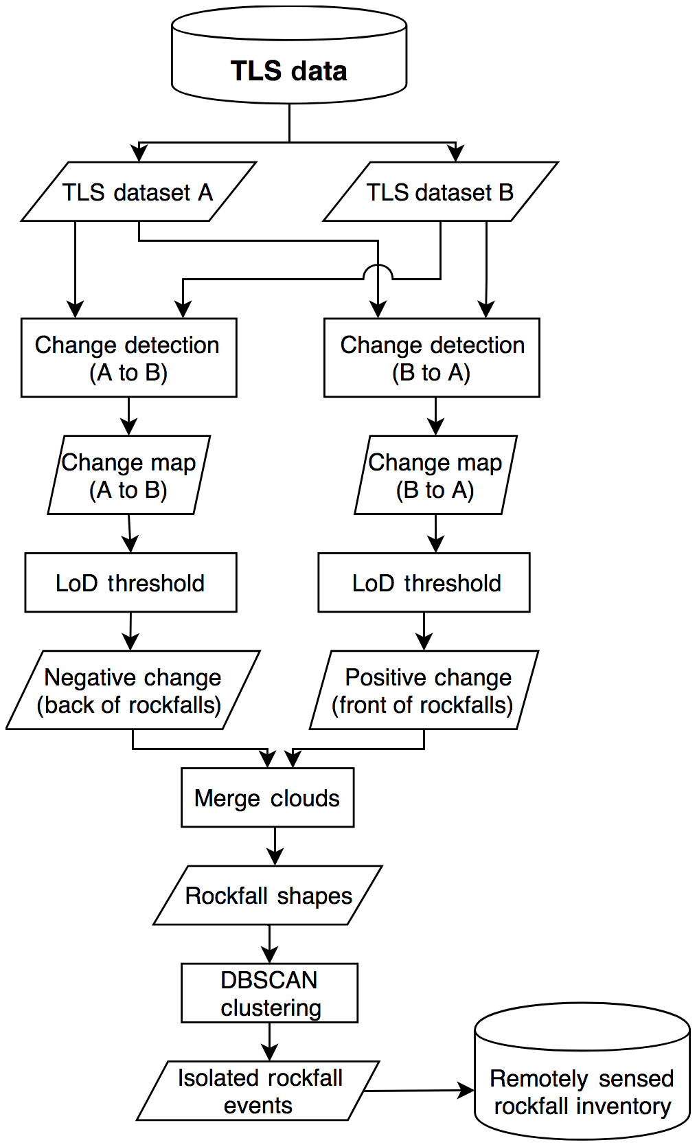
Figure 5Structured flow chart of the semi-automated process of extracting rockfall from sequential TLS scans.
The process can be summarized as follows: once the TLS scans are cleaned and aligned, the process involves computing the change between sequential scans taken at times A and B. Distances are computed from A to B and then B to A. This process determines the front and back of each rockfall event in each respective scan. A minimum change threshold is then applied; this threshold is typically based on the calculated limit of detection. The point clouds of the fronts and backs of all rockfall events are then merged to generate rockfall objects. Variants of DBSCAN (Ester et al., 1996) are then implemented to cluster individual rockfall events which have occurred between time A and B. The dimensions, volume and other parameters of each individual rockfall event can be calculated and then populated into a database for further analysis.
In this study, to compute the change between sequential TLS point clouds, the process outlined by Kromer et al. (2015) is utilized. The distance calculation is very similar to M3C2 (Lague et al., 2013), where distances are calculated along normal vectors defined by slope geometry within a specified radius from the point. The change is then filtered based on the limit of detection. The limit of detection (LOD) can be defined based on the registration error (Abellán et al., 2014). In this study, the authors take 2 times the standard deviation (95 % confidence interval) of the registration error to define the limit of detection. The LOD equates to approximately 5 cm in the summer months and 7 to 10 cm in the winter months (i.e. October to February). The higher limit of detection in the winter months corresponds to a higher standard deviation in the registration error (alignment). Higher standard deviations correspond to the winter scans, where there is generally more humidity in the air and possibly water on the slope surface, which have been found to influence the alignment process (Abellán et al., 2014).
Detectable change was then filtered based on the LOD, to resolve clusters of points that represent the scars (backs) of rockfall events. This process was repeated, conducting the change detection in the opposite direction to resolve the fronts of the rockfall objects. DBSCAN (Ester et al., 1996) was then used to cluster areas of change. The same parameters as van Veen et al. (2017) are used for the DBSCAN clustering (i.e. search radius of 30 cm and a minimum of 12 points to define a cluster).
To resolve rockfall events as opposed to debris movements, we utilized the masks mapped on the SfM-MVS photogrammetry models. The geometric centroids of each cluster are used to search and find the 10 nearest neighbours within the mask point cloud. Based on the classification of the 10 nearest neighbours within the mask point cloud, a vote is conducted to classify the centroid as either a debris movement or rockfall depending on the mask classification (i.e. bedrock vs. channel).
2.4 Model fitting
The following subsections present the background for each of the models used to determine the dimensions of the rockfall objects. Each of the approaches were implemented in MATLAB (Mathworks, 2018).
2.4.1 Bounding box
A bounding box or enclosing box defines the minimum extents of a box within which all points are contained. In this study, the bounding box is oriented with the edges of the calculated box parallel to the Cartesian coordinate axes (Fig. 6a).
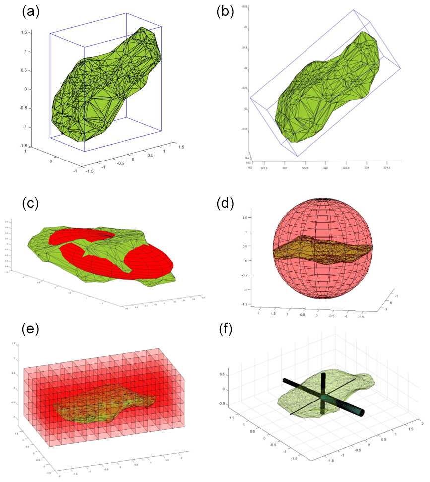
Figure 6Visual representation of each of the model fitting methods used in the study. (a) Bounding box approach (e.g. van Veen et al., 2017; Benjamin, 2018; Williams, 2017). (b) Adjusted bounding box approach. (c) Least-squares ellipsoid fit. (d) Minimum bounding sphere fit. (e) RFSHAPZ approach. (f) RFCYLIN approach.
2.4.2 Adjusted bounding box
The adjusted bounding box approach differs from the bounding box approach in that the orientation of the box is not subjected to any constraints. In this study, singular value decomposition (SVD) (Golub and Loan, 1996) is used to determine the orientation of the object relative to the principal axes in Cartesian space. SVD is used because this process can handle any m×n matrix, whereas eigenvalue decomposition can only be applied to certain classes of square matrices (Golub and Loan, 1996). The direction of most variance using SVD is determined and the point cloud is rotated to align with the direction of maximum variance with the x axis in Cartesian space. This results in the x axis of the box being aligned with the longest dimension of the object. A bounding box can then be calculated for the point cloud (Fig. 6b).
2.4.3 Least-squares ellipsoid
An ellipsoid can be defined as a closed quadric surface that is the analogue of an ellipse. To fit an ellipsoid to the point cloud defining a rockfall object, an algebraic form linear-least-squares ellipsoid fit (Schneider and Eberly, 2003) is implemented. An algebraic fitting model was selected as opposed to an orthogonal fitting ellipsoid to reduce computing time and to benefit from the advantages of solving linear-least-squares problems (Li and Griffiths, 2004). The algorithm generates a least-squares ellipsoid fit of the input point cloud (Fig. 6c). Further details on the algorithm and derivation can be found in Schneider and Eberly (2003).
2.4.4 Minimum bounding sphere
To fit a minimum bounding sphere to the point cloud, Welzl's 1991 algorithm is implemented. The algorithm computes the smallest sphere enclosing a set of points in 3-D space in linear time (Fig. 6d). For further details on the algorithm, readers are referred to Welzl (1991).
2.4.5 RFSHAPZ
In this study, the RFSHAPZ (rockfall shape) approach is introduced. The approach can be broken into four main steps: (1) point cloud preparation, (2) voxelation, (3) distance calculations, and (4) curve fitting. Figure 7 outlines a flowchart for the process used to determine the dimensions of each rockfall object.
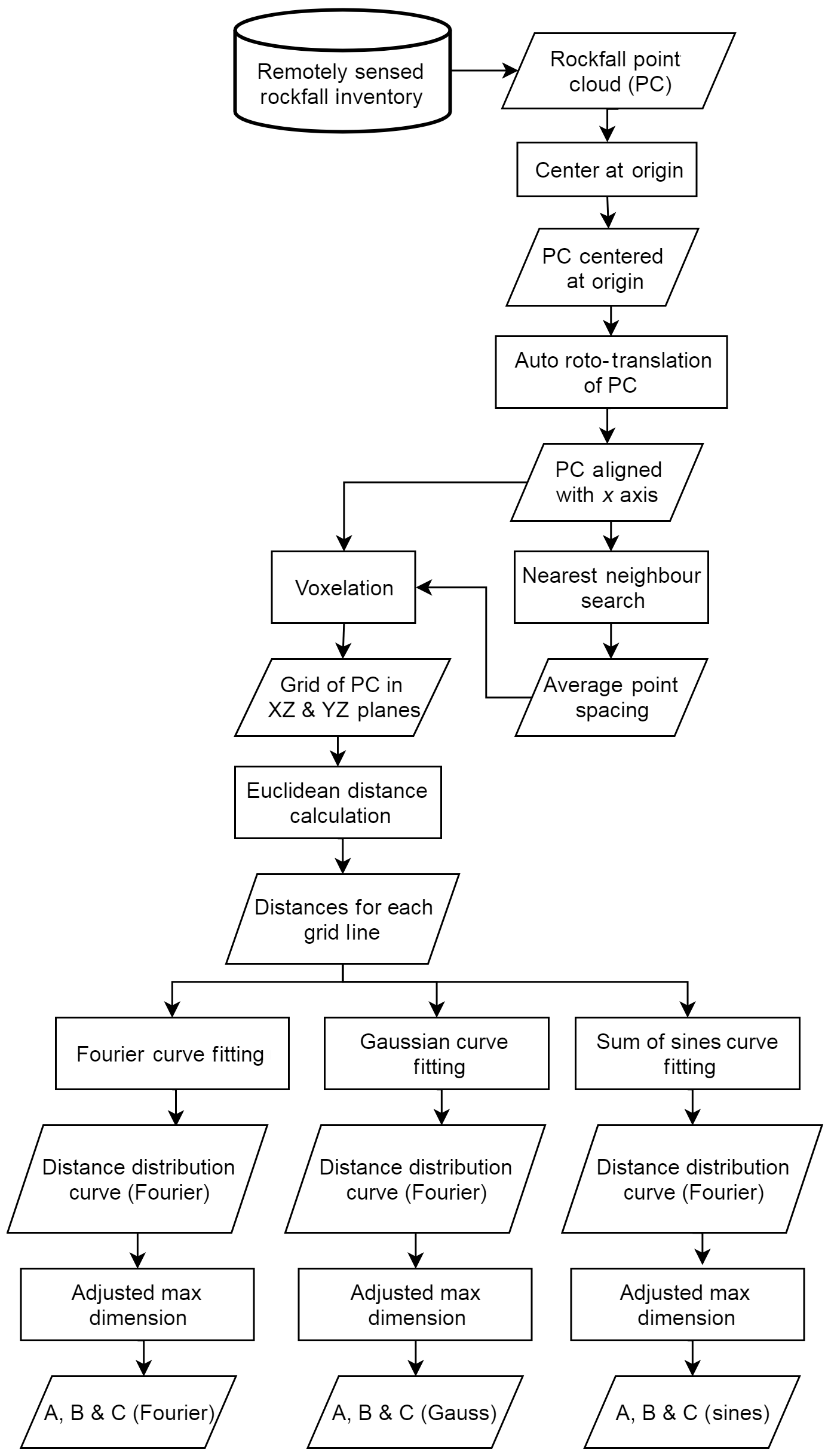
Point cloud preparation involves translating each rockfall object so that the object's geometric centroid is centered at the origin of a locally defined Cartesian coordinate system. Once the object is centered at the origin, SVD is used to rotate the object so that the longest dimension is parallel with the x axis in Cartesian space.
The next step involves generating a voxel grid of the point cloud. A voxel is a 3-D volume element that represents a numerical value. For this study, the default voxel cube size is defined as a function of the point spacing. We calculate the average point spacing of the surfaces that make up the rockfall object and then double the value to determine the voxel size. The size of the voxel is therefore a function of the point spacing and can be adjusted depending on the rockfall object. The voxel grid is used to provide a spatial context for the rockfall object and allows all points within each voxel to be stored for further analysis. Once the voxel grid is established, for each voxel grid line in the XY and XZ planes, we calculate the maximum Euclidean distance between points within populated voxels (Fig. 6e). The calculated distances are plotted along each grid line. Curves are then fit to each of the distributions, utilizing a Fourier series fit, a Gaussian fit and a sum of sines fit. An overview of each of the fitting methods is provided below.
The Fourier series is a sum of sine and cosine functions that describes a periodic signal. In this study, we use the trigonometric form of the series which can be expressed as
where a0 is a constant term and is associated with the i=0 in the cosine term. w represents the fundamental frequency of the signal, and n is the number of terms in the series. For this study, n is fixed at a constant value of one.
The Gaussian model fits peaks in a data series and is given by
where a is the amplitude, b is the centroid (location), c is related to the peak width and n is the number of peaks to fit. For this study, n is fixed at a value of one.
The last curve fitting function used is the sum of sines model. This model fits periodic functions and is given by
where a is the amplitude, b is the frequency and c is the phase constant for each sine wave term. n defines the number of terms in the series. This equation is closely related to the Fourier series described in Eq. (4). The main difference is that the sum of sines equation includes the phase constant and does not include a constant (intercept) term. For this study, n is fixed at a value of one.
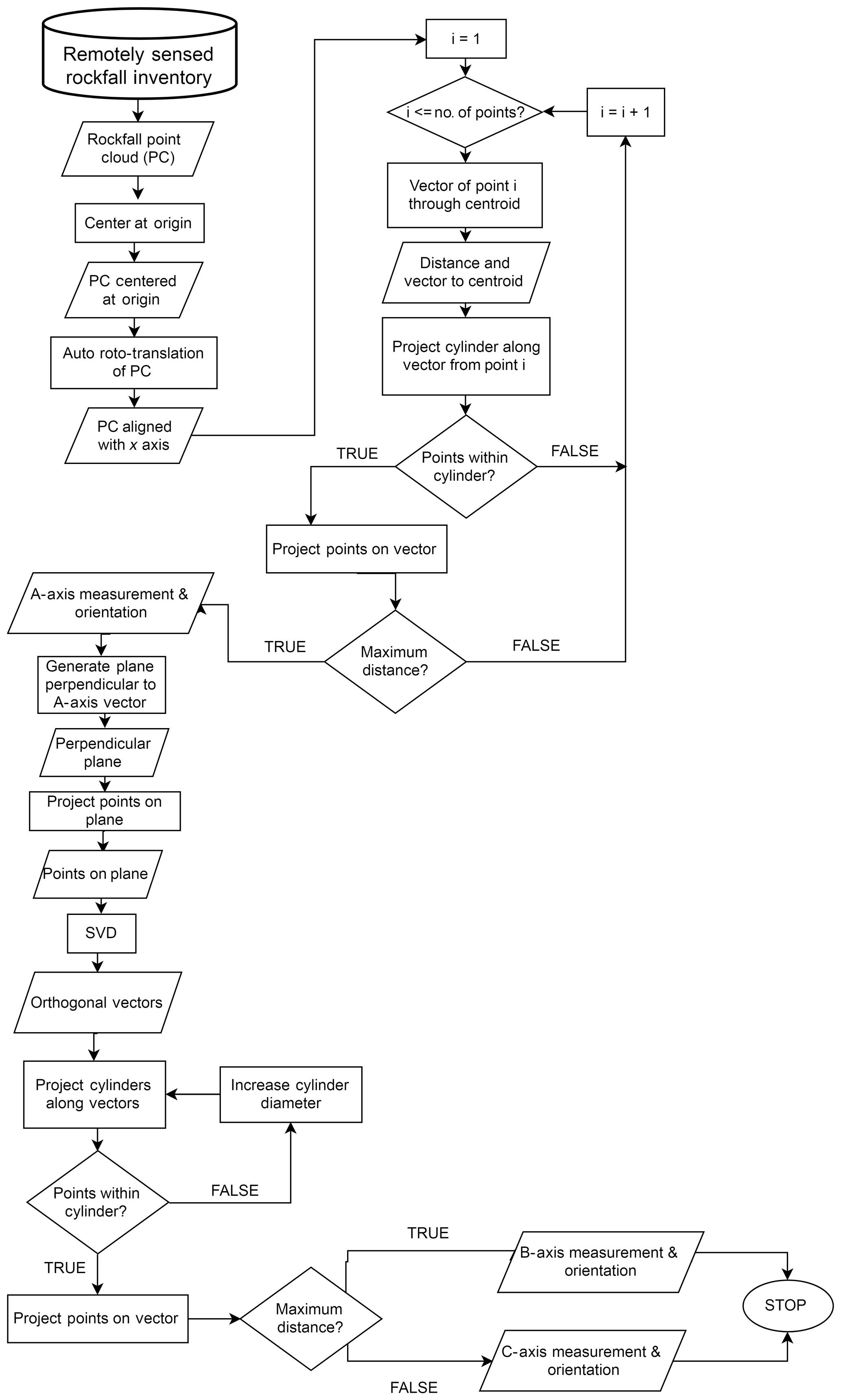
2.4.6 RFCYLIN
The last approach introduced and implemented in this study, RFCYLIN (rockfall cylinders), draws inspiration from the M3C2 methodology (Lague et al., 2013). The point cloud preparation is the same as is described for the RFSHAPZ approach discussed in Sect. 2.4.5.
For all points in the cloud defining the rockfall object, we calculate the vector and Euclidean distance from each point to the geometric centroid. The vector is oriented towards the calculated centroid. A cylinder is then projected from each point through the geometric centroid of the rockfall object. The length of the cylinder is set to be greater than the distance calculated between each point and the geometric centroid. After the cylinder has been projected, points are found to be within the cylinder. These points are projected on the vector line, and the maximum distance between all points through the centroid is determined. This process results in determining the maximum (longest) dimension of the rockfall object.
Once the maximum distance and vector orientation has been calculated, orthogonal vectors to the vector of maximum distance are then calculated through SVD. To do this step, a plane is projected perpendicular to the vector defining the maximum dimension. Points defining the rockfall object are projected onto the plane. SVD is then used to determine the direction of maximum and minimum variance. These define the vector orientations of the other axes. Once the orientations of the orthogonal vectors have been determined, cylinders are projected along each vector to find points which lie within the cylinder. If no points are found to be within the cylinder, we incrementally increase the diameter of the cylinder until points are found to be within the cylinder. These points are then projected onto the vector line defining the centerline of the cylinder. The distances between points along each of the orthogonal vectors are calculated and define the intermediate and shortest dimensions of the rockfall object (Fig. 6f). A flowchart outlining this algorithm is displayed in Fig. 8.
The calculated dimensions of the rockfall objects, using each of the techniques described in Sect. 2, are tabulated for analysis. Section 3.1 presents the results from the analysis of the synthetic block dataset. Section 3.2 presents the results of the analysis on the rockfall objects extracted from the TLS monitoring in the White Canyon.
3.1 Synthetic block dataset
The dimensions of the 20 synthetic blocks described in Sect. 2.1 were measured using the six methods outlined in Sect. 2.4. In addition, independent sets of measurements were made manually by two different members of the research team.
The calculated dimensions were plotted on Sneed and Folk ternary diagrams in order to examine the geometric results, as shown in Fig. 9. The data for the smooth (rounded) and angular synthetic objects are shown on separate diagrams to highlight differences in the distribution of these datasets. The observations made of these datasets include the following.
-
The angular synthetic block dataset displayed the largest spread in the geometry represented by the calculated dimensions, when compared to the smooth rockfall objects.
-
The measured dimensions of the very bladed and very elongate blocks, at the bottom left and right corners of the ternary diagram respectively, were closely aligned for all methods and manual measurements.
-
The angular compact series (i.e. compact platy, compact bladed and compact elongate) showed the greatest divergence between the manual measurements and the automated methods. A number of the methods, including the manual measurements, classified the angular compact-platy block as platy. The methods which did correctly categorize this shape include the bounding box, the adjusted bounding box, the RFSHAPZ Gaussian fit and the manual measurements. These measurements, however, are not closely aligned and display significant spread between the data points.
-
With increasing compactness of the synthetic shapes, there are challenges with assessing what is the shortest axis with manual measurements. This effect is compounded with increasing angularity of the rockfall object.
-
For the angular compact-elongate block, the two manual measurements incorrectly classify the block as compact bladed while all of the calculated dimensions classify the block as compact elongate.
The results of the rounded synthetic block dataset displayed significantly less spread in the calculated and measured block dimensions relative to their angular counterparts. Only the rounded compact-elongate block had classification issues based on the measured or calculated dimensions. The RFCYLIN approach, RFSHAPZ and adjusted bounding box all classified the block as compact bladed.
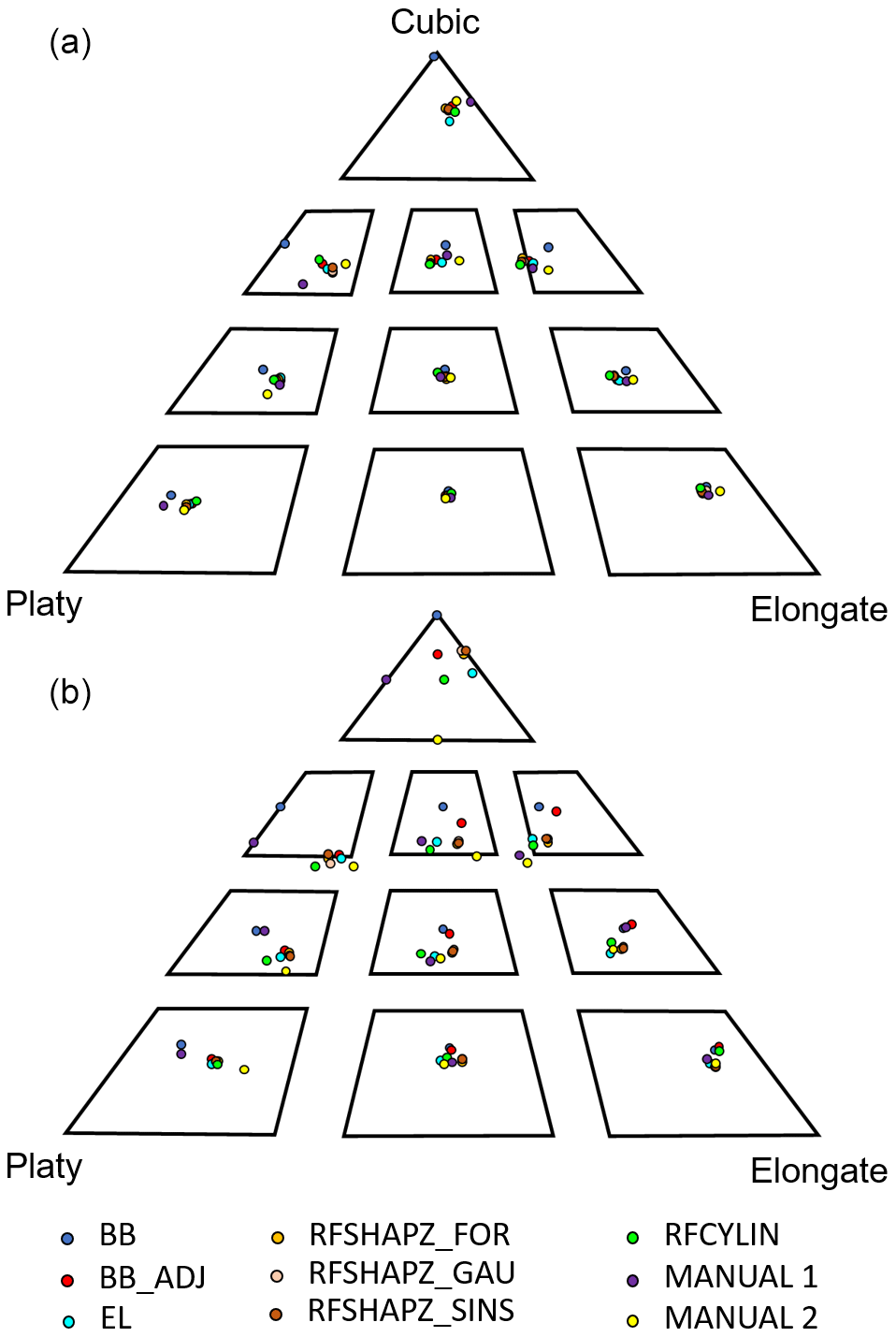
Figure 9Sneed and Folk ternary diagrams separated to highlight shape classification results. (a) The results of each of the nine fits for each of the rounded synthetic blocks. (b) The results of each of the fits for the angular synthetic blocks. BB: bounding box; BB_ADJ: adjusted bounding box; EL: least-squares ellipsoidal fit; RFSHAPZ_FOR: RFSHAPZ Fourier fit; RFSHAPZ_GAU: RFSHPZ Gaussian fit; RFSHAPZ_SINS: RFSHAPZ sum of sines fit; RFCYLIN: RFCYLIN fit.
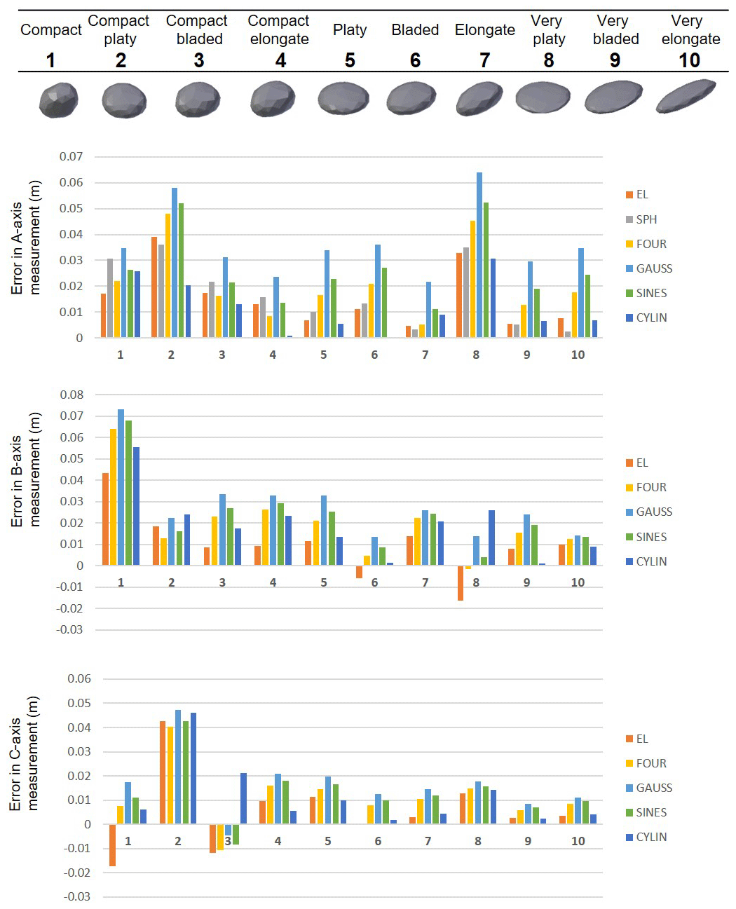
Figure 10Error in dimension measurement for each fit compared to a set of manual measurements for the rounded synthetic blocks. EL: least-squares ellipsoidal fit; FOUR: RFSHAPZ Fourier fit; GAUSS: RFSHPZ Gaussian fit; SINES: RFSHAPZ sum of sines fit; CYLIN: RFCYLIN fit.
In order to analyze the results, the manual measurements were selected as a basis of comparison with the synthetic blocks. Figure 10 displays the results for the rounded synthetic blocks, and Fig. 11 presents the results for the angular set. The bounding box and adjusted bounding box approaches were excluded from this analysis since they are a component of the process of how the synthetic blocks were generated within Blender (Sala, 2018).
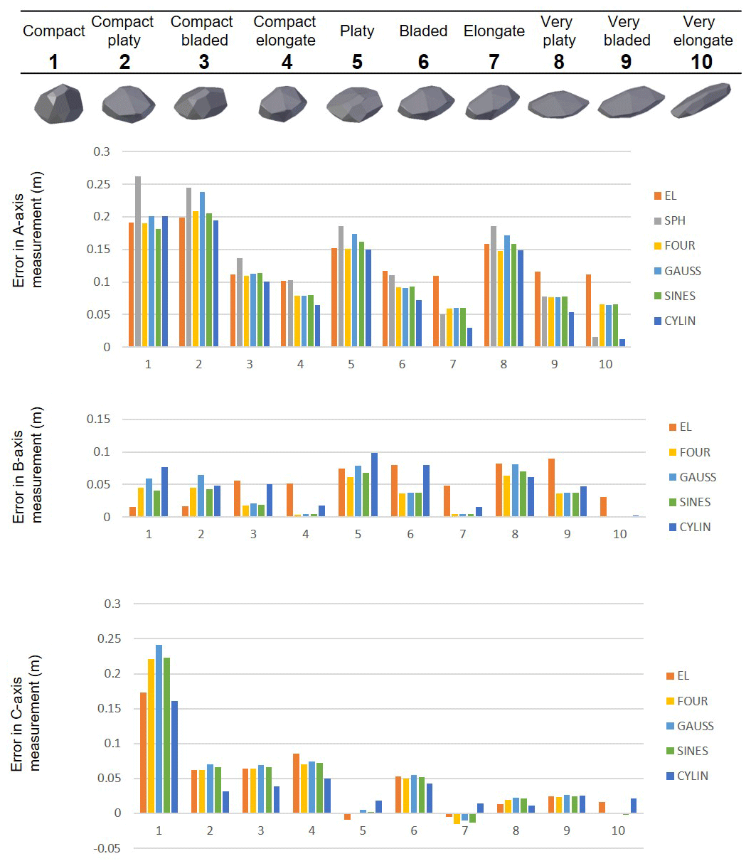
Figure 11Error in dimension measurement for each fit compared to a set of manual measurements for the angular synthetic blocks. SPH: minimum-bounding sphere fit; EL: least-squares ellipsoidal fit; FOUR: RFSHAPZ Fourier fit; GAUSS: RFSHPZ Gaussian fit; SINES: RFSHAPZ sum of sines fit; CYLIN: RFCYLIN fit.
Overall, the errors associated with the angular dataset are an order of magnitude higher than the rounded dataset (A axis). In addition, none of the calculated fits underestimated the A-axis dimension for both the angular and rounded datasets. Relative to the rest of the shapes, the platy series (i.e. compact platy, platy, very platy) showed the highest deviations from the manual measurement. Within the angular data series, errors on the order of 20 cm (∼20 %) were reported for the A-axis measurement.
3.2 White Canyon rockfall dataset
The White Canyon (50.266261∘, −121.538943∘), located in the Thompson Rail Corridor in Interior British Columbia, Canada, is an operationally challenging rock slope (Fig. 2). Rockfall and the movement of debris originating from the steep slopes present hazards to the safe operation of the Canadian National (CN) rail line, which runs at the base of the slope adjacent to the Thompson River (Bonneau and Hutchinson, 2017; Kromer et al., 2015; van Veen et al., 2017).
The morphology of the White Canyon is highly complex; differential erosion has formed a morphology which varies across the canyon and consists of vertical spires and deeply incised channels. The active portion of the canyon reaches up to 500 m in height above the railway track. The canyon spans approximately 2.2 km between mile 093.1 and 094.6 of the CN Ashcroft subdivision. A series of short tunnels mark the entrances to the canyon; a tunnel can be found on either side of the canyon. A third short tunnel is located in the middle of the canyon through a ridge which separates the eastern and western portions of the site.
Two dominant geological units comprise the geology of the White Canyon. The primary unit is the Lytton Gneiss. The Lytton Gneiss is a quartzofeldspathic gneiss with amphibolite bands, containing massive quartzite, amphibolite and gabbroic intrusions (Monger, 1985). In the most western extent of the canyon towards the west tunnel portal is the other dominant unit, the Mt. Lytton batholith. The Mt. Lytton batholith is a distinctly red stained unit which is composed of granodiorite with local diorite and gabbro. The red staining of the rock mass is thought to be a direct result of fluids originating from the weathering of hematite in overlying mid-Cretaceous continental clastic rocks. Two sets of dykes have intruded the Lytton Gneiss within the White Canyon. The first dyke set consists of tonalitic intrusions which are believed to be related to the emplacement of the Mt. Lytton batholith (Brown, 1981). The second dyke set is a series of dioritic intrusions which cross-cut the Lytton Gneiss and tonalitic dykes. These dioritic intrusions are believed to be part of the Kingsvale andesites (Brown, 1981).
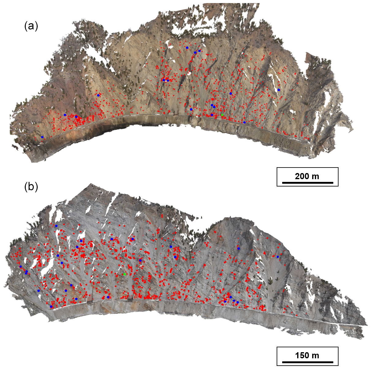
Figure 12The White Canyon rockfall database. The centroid of each rockfall event is displayed as a red dot on the photogrammetry model. The blue dots correspond to the 50 rockfall events analyzed in detail. The light green dots correspond to the events analyzed in Fig. 14. (a) White Canyon West results. (b) White Canyon East results.
Analysis of the TLS data collected at the White Canyon study slope between November 2014 and December 2017 using the semi-automated rockfall extraction process resulted in a database of 4960 rockfall events: 2566 events in WCW and 2394 events in WCE. The centroid of each of the detected rockfalls is displayed in Fig. 12. The data plotted in this figure display that the spatial distribution of rockfall is quite varied across the entire canyon. Rockfalls were documented to occur in all lithologies present in the slope.
A subset of rockfall events were identified and selected from the overall database for further analysis. The volumes of the selected rockfalls ranged from 1 up to 130 m3, which was the largest event recorded during this period. As a first pass, only events larger than 1 m3 were selected from the full database. This selection was based on a criterion in CN's Rockfall Hazard Rating System (RHRS: Abbott et al., 1998) which focuses on the rockfall events that are greater than 1 m3. The resulting 160 rockfall events were considered large enough that a reasonable estimate of their shape could be made from the point cloud where the data points are spaced at approximately 7 cm apart. A total of 110 rockfall events were removed from the subset due to their shapes. It is probable that numerous smaller failures have occurred from that same location (van Veen et al., 2017; Williams et al., 2018) during the 3 to 4 months elapsed time between scanning campaigns. The change detection, therefore, will generate the geometry of an apparent single rockfall which is in fact likely to be the result of several coalesced smaller events, resulting in complex, multi-lobed shapes. With more frequent scanning intervals, the authors would have more confidence that these rockfalls are single events or multiple coalescing events. The remaining 50 events were large enough to be of potential impact on the railway infrastructure and were interpreted to be the result of discrete individual events, based on fairly well constrained shape, relative to rock mass structure present at the rockfall source location. Using the six methods outlined in Sect. 2.4, the dimensions of the 50 blocks were measured. In addition to the automated measurements, two sets of independent manual measurements were also made.

Figure 13Sneed and Folk ternary diagrams for each of the model fits for the 50 rockfall events that occurred in the White Canyon. The bar chart at the bottom highlights the percentage of classes for each of the fits. BB: bounding box; BB_ADJ: adjusted bounding box; EL: least-squares ellipsoidal fit; FOUR: RFSHAPZ Fourier fit; GAUSS: RFSHPZ Gaussian fit; SINES: RFSHAPZ sum of sines fit; RFCYLIN: RFCYLIN fit.
Figure 13 displays the Sneed and Folk ternary diagram for each model fit applied to the 50 rockfall cases in the White Canyon. The bounding box approach resulted in a distribution on the Sneed and Folk ternary diagram that is quite scattered; however, the overall trend is towards a more cubic shape for all of the measured rockfall objects. All possible shapes in the Sneed and Folk classification (i.e. compact, very elongate) are represented by rockfall object shapes assessed using this method.
The results of the other fitting methods and the manual measurements are in stark contrast to the results of the bounding box approach. None of the other fitting methods or manual measurements classify any of the 50 rockfall events as cubic or in the compact series (i.e. compact platy, etc.). All the other fitting methods and manual measurements trend towards very bladed to very elongate shape classifications and are distributed across the lower portion of the diagram.
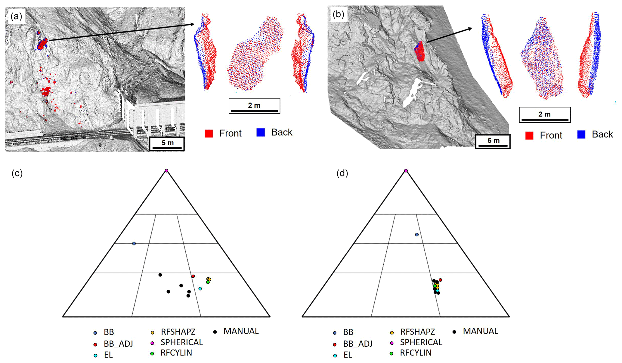
Figure 14Overview of the two rockfall events analyzed in more detail, with manual measurements made by five different people. (a) The spatial location and shape of the rockfall event in White Canyon West. The red points correspond to the front of the object while the blue points correspond to the back of the object. (b) The spatial location and shape of the rockfall event in White Canyon East. The red points correspond to the front of the object while the blue points correspond to the back of the object. (c) The results of the different fitting methods for the rockfall event shown in panel (a). (d) The results of the different fitting methods for the rockfall event shown in panel (b). BB: bounding box; BB_ADJ: adjusted bounding box; EL: least-squares ellipsoidal fit.
Two rockfall events were isolated from the 50 events to illustrate the complexities inherent in working with real rockfall shapes, as well as the variations in the calculated dimensions (Sneed and Folk shape classification) using each of the methods implemented in the study (Fig. 14). A notch in one of the rockfalls (Fig. 14a) gives one of the objects more geometric complexity than its counterpart (Fig. 14b). For the geometrically complex object, the results of the rockfall event dimension measurements are displayed in Fig. 6. The rockfall occurred in the western portion of the White Canyon between June 2015 and August 2015. The rockfall fell from a height of approximately 20 m above track level, and a number of impact points along the rockfall trajectory were documented from the change detection analysis. The volume of the rockfall event was estimated to be approximately 1.7 m3, and the shape, although complex, is considered to be well enough constrained that this could be the result of a single event that occurred during that 3-month period between scans. The other rockfall event analyzed (Fig. 14b) occurred in the eastern portion of the White Canyon between October 2015 and February 2016. This 1 m3 rockfall occurred above a debris channel in the quartzofeldspathic gneiss host unit. Based on the orientation and spacing of the discontinuities in the surrounding rock mass, it is thought that this event is likely the result of a single event that occurred between the scan dates.
Five different independent manual measurements of the dimensions were conducted for both of these rockfall objects. For the first object (Fig. 14a), all of the manual measurements indicated that the rockfall object is classified as very bladed. The adjusted bounding box, least-squares ellipsoid, RFSHAPZ fits and the RFCYLIN approach all resulted in the rockfall object being classified as very elongate. The bounding box classified the rockfall object as either compact platy or platy. The spherical fit, as always, classified the rockfall object as compact. This is a direct result of the fact that all calculated dimensions are equal when using the spherical fit.
In comparison, the less complex object was classified as very elongate with all manual measurements and the adjusted bounding box, least-squares ellipsoid, RFSHAPZ fits and the RFCYLIN approach. The bounding box approach resulted in the object being classified as compact bladed, and the spherical fit classified the rockfall object as compact.
In general, when comparing the shape classifications of the dataset of the 50 rockfall objects to the manual shape classifications, there were significant differences. When the automated shape classifications were compared to the Manual 1 and Manual 2 shape classifications, the bounding boxing agreed with Manual 1 and Manual 2 in 3 of the 50 cases. The adjusted bounding box, ellipsoid fit, each of the RFSHAPZ fits (Fourier, Gaussian and sum of sines) and RFCYLIN agreed with the Manual 1∕2 shape classifications in 29∕25, 25∕29, 29∕30, 29∕29, 28∕30 and 24∕29 of the cases, respectively.
Interestingly, there were only 34 cases where the shape classifications of the two manual measurements agreed with one another. Furthermore, there were only 8 cases of the 50 analyzed where both manual measurements matched all of the automated approaches, excluding the bounding box and spherical fits. Neither of the two manual classification datasets aligned with any of the spherical fits.
The shape or form of an object can be classified by assessing aspect ratios of major axes. However, it has been noted that there is no standardized method used to determine axis length or if the axis measurements should be orthogonal or not. Additionally, there is an inherent ambiguity in selecting the geometric axes of a particle (Blott and Pye, 2008). The ambiguity arises with increasing compactness of particles, where all axes lengths are almost equal. In these situations, it is very difficult as well as subjective as to how these dimensions are measured since it is difficult to manually define an orthogonal frame. In this study, the authors have presented and compared six different methods for assessing a rockfall object's dimensions and resulting shape. All of the algorithms have been presented, allowing these approaches to be replicated for future works. In addition, the authors have created a synthetic dataset of rockfall objects that can be used to assess new algorithms aimed at determining a rockfall object's dimensions. This synthetic dataset represents a step forward in standardizing methodologies for best practice in generating remotely sensed rockfall inventories.
The results of this study confirm that the method in which dimensions are measured results in significantly different shape classifications. The authors have demonstrated that a bounding box approach (e.g. van Veen et al., 2017; Benjamin, 2018) can potentially bias the dimension measurements toward a more cubic form, if the orientation of the longest axis of the rockfall object is not parallel with one of the major Cartesian axes. If opting for a bounding box approach to determine the object's dimensions, the adjusted approach should be used instead.
A minimum bounding sphere was shown to be highly inappropriate for dimension extraction in the cases analyzed in this work. The approach results in all dimensions of the object being equal and every single object being classified as compact or equant (i.e. ). This may be valid for rockfall objects in some narrowly defined geological settings where equant blocks are released by the slope rock mass. For example, further work is required to assess the applicability of the minimum bounding sphere approach to determine the dimensions of detached and rounded cobbles and boulders from select horizons of postglacial river terraces (Bonneau and Hutchinson, 2018, 2019).
In comparison to the other methods, the RFCYLIN approach introduced in the study is the most computationally demanding algorithm. The method tries to standardize an approach to measure dimensions, where each axis is measured orthogonally to one another after the longest dimension has been defined. However, occlusions and edge effects in change detection analysis can result in inaccurate distance calculations that can compound when trying to quantify the object's dimensions. Therefore, while this method most closely aligns with the definition of measuring three mutually orthogonal axes, it is sensitive to data occlusions. In comparison to the RFCYLIN, the adjusted bounding box approach guarantees that the maximum dimensions will be measured. Therefore, this method is sensitive to outlier points, whereby the maximum extent of complex geometry is defined using this approach. The RFSHAPZ approach attempts to bypass these complications by utilizing curve fitting approaches to assess the object dimensions when there is non-uniform distribution of point density. This approach will not result in the maximum dimensions being selected but rather representative dimensions based on the input point cloud. In comparison to the other methods, this method is the second most computationally demanding algorithm. The bounding box and adjusted bounding boxes are the least computationally demanding of the presented approaches. The adjusted bounding box is a robust approach that would work well in all environments when the input point clouds do not contain outlier points. When the input point clouds contain a uniform distribution of points, at the cost of some increased computational time, the RFCYLIN approach remains the closest to the definition of three mutually orthogonal axes based on the input point cloud.
Automated approaches have several advantages over manually classifying the dimensions of rockfall objects for a shape analysis. An automated approach removes the subjectivity that could potentially be induced by manually measuring an object. Increasing angularity or complex geometric features in the shapes can make it increasingly difficult to define orthogonal measurements for both manual and automated approaches. In comparison to manual measurements, however, an automated approach is repeatable because there is inherent subjectivity in the manual measurements depending on the skill and experience of the person doing the work. In this work, the two independent sets of manual measurements for the White Canyon dataset differed depending on the complexity of the object. The classification resulting from the manual methods agreed in only 34 of the 50 analyzed cases.
In the interpretation of the results, it should be noted that there are hard cut-offs between the different classes in the Sneed–Folk diagram. This can lead to circumstances where the object plots directly on the line between two classes yet is assigned a single shape class.
Almost all the automated fits attempt to find the maximum distance in order to define one of the dimensions, except the RFSHAPZ approach. In comparison to the manual measurements, the measured dimension could be reflective of the overall dimension as opposed to the maximum. As illustrated with the case study of the synthetic objects, with increasing angularity and compactness, there is greater difficulty in defining the shortest axis of the objects. Underestimation of the shortest axis will result in the objects being classified as flatter shapes, while overestimation leads to classification in a more compact class.
Assessing the overall dataset of the 50 rockfall objects from the White Canyon, the shape classes trend toward very elongate to very bladed. This is the direct result of the orientations of the joint sets and foliation within the rock mass which promotes the generation of these shapes. This result is in contrast to work previously done on this slope by van Veen et al. (2017), where the rockfall shapes were mostly cubic: this is a direct result of the bounding box approach implemented in their study.
The differences in shape classification have direct implications for rockfall modelling. The size and shape of rock blocks are vital components when considering and assessing potential runout trajectories. Shape has been noted to affect the degree to which rolling can be sustained for blocks (Kobayashi et al., 1990). Furthermore, the degree of angularity of a block also has implications for transitions between translational and rotational motion (Pfeiffer and Bowen, 1989).
Industry standard rockfall modelling software packages such as RockyFor3D (Dorren, 2016) still use relatively simple geometric shapes (rectangles, ellipsoids, spheres). Therefore, if we consider the simulation of a cuboid or rectangular prism, where the volume can be defined as a product of the three axes, the measured dimensions directly influence the volume of the rockfall being simulated. The volume then defines the mass of the object and, as a result, the moment of inertia.
In this study, the authors have demonstrated that the method used to measure the dimensions of rockfall objects matters. Depending on the method used, the object's shape may be misclassified into non-representative geometric categories. The classification of shape has implications for the assessment of rockfall hazards when using shape classifications as input to rockfall modelling. Therefore, it is imperative to select a robust method that can accurately and efficiently determine the dimensions of a rockfall object.
As illustrated with the analysis of synthetic blocks, increasing compactness and angularity results in the most difficulties in measuring the dimensions of a rockfall object. All automated methods and manual measurements displayed less scatter for the rounded dataset in comparison to their angular counterparts. Furthermore, there is a decrease in differences between the calculated dimensions as the object becomes less compact. This is best illustrated with the synthetic very bladed and very elongate blocks. The dimensions of both the angular and rounded version resulted in minimal scatter in the calculated dimensions. The differences between the lengths of the long, intermediate and short axes for these blocks are quite apparent. Therefore, both the manual and automated methods can converge on a dimension length and are not subject to the uncertainties created when there are similarities in the length of two or three of the axes.
The shapes of real rockfall objects are quite complex, as displayed with the White Canyon dataset, where the results of the different axis measuring methods were quite variable. Angularity, non-uniform point spacing and occlusion in the rockfall object point clouds results in complications for extracting dimensions with both manual and automated methods. From the analysis of 50 rockfall events in the White Canyon, it appears that the RFSHAPZ method most closely aligns with the manual measurements (Fig. 13). However, a comparison between the manual measurements shows that these measurements are different. The manual method relies on the user consistently determining a representative length, as opposed to automated methods which attempt to find the length of the maximum dimension.
The adjusted bounding box is the most robust approach presented in this study; however, the results can be sensitive to outlier points, leading to a potentially significant over estimation of the block volume, particularly for complex objects. The bounding box approach should not be used in any future studies. The two methods introduced in this study, RFCYLIN and RFSHAPZ, were designed to standardize the way in which the dimensions are measured and work around challenges such as non-uniform point density and increasing angularity, while staying most closely aligned with the definition of measuring three mutually orthogonal axes. These two methods are, however, the most computationally demanding of all the presented approaches.
The underlying research data for this project can not be made publicly available as they are commercially sensitive and permission must be granted by our industry partners to access the data.
DAB coordinated the study, generated all algorithms and code, and drafted the manuscript. DAB and DJH co-analyzed the data. MC and PMD ran the code. ZS generated the synthetic block dataset. All co-authors reviewed and edited the manuscript.
The authors declare that they have no conflict of interest.
Past and present Queen's RGHRP team members are thanked for their help with data collection. The comments and suggestions by two anonymous reviewers are gratefully acknowledged.
This research has been supported by the Natural Sciences and Engineering Research Council of Canada Discovery Grant (grant no. 05668), Collaborative Research and Development (CRD; grant no. 470162), and the NSERC Graduate Scholarship Program.
This paper was edited by Andreas Günther and reviewed by two anonymous referees.
Abbott, B., Bruce, I., Savigny, W., Keegan, T., and Oboni, F.: A Methodology for the Assessment of Rockfall Hazard Risk along Linear Transportation Corridors, 8th International Association of Engineering Geology Conference, A Global View from the Pacific Rim, 21– 25 September 1998, Vancouver, BC, Canada, 1998.
Abellán, A., Oppikofer, T., Jaboyedoff, M., Rosser, N. J., Lim, M., and Lato, M. J.: Terrestrial laser scanning of rock slope instabilities, Earth Surf. Proc. Land., 39, 80–97, https://doi.org/10.1002/esp.3493, 2014.
Agisoft LLC: Agisoft PhotoScan User Manual, St. Petersburg, Russia, available at: https://www.agisoft.com/, last access: 29 May 2018.
Benjamin, J.: Regional-scale controls on rockfall occurrence, PhD Thesis, Durham University, Durham, UK, 2018.
Besl, P. and McKay, N.: A Method for Registration of 3-D Shapes, IEEE T. Pattern Anal., 14, 239–256, https://doi.org/10.1109/34.121791, 1992.
Blender: Blender – a 3D modelling and rendering package, available at: http://www.blender.org, last access: 12 July 2018.
Blott, S. J. and Pye, K.: Particle shape: A review and new methods of characterization and classification, Sedimentology, 55, 31–63, https://doi.org/10.1111/j.1365-3091.2007.00892.x, 2008.
Bonneau, D. A. and Hutchinson, D. J.: Applications of Remote Sensing for Characterizing Debris Channel Processes, in: Landslides: Putting Experience, Knowledge and Emerging Technologies into Practice., edited by: De Graff, J. V. and Shakoor, A., Association of Environmental & Engineering Geologists (AEG), Roanoke, USA, 748–759, 2017.
Bonneau, D. A. and Hutchinson, D. J.: The Use of Multi-Scale Dimensionality Analysis for the Characterization of Debris Distribution Patterns, in: Geohazards 7 – Engineering Resiliency in a Changing Climate, p. 8, Canmore, Alberta, Canada, 2018.
Bonneau, D. A. and Hutchinson, D. J.: The use of terrestrial laser scanning for the characterization of a cliff-talus system in the Thompson River Valley, British Columbia, Canada, Geomorphology, 327, 598–609, https://doi.org/10.1016/j.geomorph.2018.11.022, 2019.
Brown, D. A.: Geology of the Lytton Area, British Columbia, BSc Thesis, Carleton University, Ottawa, Canada, 1981.
Carrea, D., Abellan, A., Derron, M. H., and Jaboyedoff, M.: Automatic Rockfalls Volume Estimation Based on Terrestrial Laser Scanning Data, in: Engineering Geology for Society and Territory – Volume 2: Landslide Processes, edited by: Lollino, G., Giordan, D., Crosta, G. B., Corominas, J., Azzam, R., Wasowski, J., and Sciarra, N., Springer International Publishing, Cham, Switzerland, 1–2177, 2015.
Cloutier, C., Locat, J., Geertsema, M., Jakob, M., and Schnorbus, M.: Potential impacts of climate change on landslides occurrence in Canada, in: Slope Safety Preparedness for Impact of Climate Change, edited by: Ho, K., Lacasse, S., and Picarelli, L., CRC Press, CRC Press/Balkema, Leiden, the Netherlands, 71–104, https://doi.org/10.1201/9781315387789-3, 2016.
Dorren, L. K. A.: Rockyfor3D (v5.2) Revealed – Transparent Description of the Complete 3D Rockfall Model, Geneva, Switzerland, available at: http://www.ecorisq.org (last access: 27 July 2018), 2016.
Dussauge, C., Grasso, J.-R., and Helmstetter, A.: Statistical analysis of rockfall volume distributions: Implications for rockfall dynamics, J. Geophys. Res.-Sol. Ea., 108, 2286, https://doi.org/10.1029/2001JB000650, 2003.
Ester, M., Kriegel, H.-P., Sander, J., and Xu, X.: A Density-Based Algorithm for Discovering Clusters in Large Spatial Databases with Noise, in: Knowledge Discovery and Data Mining 1996, Elsevier, Portland, Oregon, USA, 226–231, 1996.
Froude, M. J. and Petley, D. N.: Global fatal landslide occurrence from 2004 to 2016, Nat. Hazards Earth Syst. Sci., 18, 2161–2181, https://doi.org/10.5194/nhess-18-2161-2018, 2018.
Glover, J.: Rock-shape and its role in rockfall dynamics, PhD Thesis, Durham University, Durham, UK, 2015.
Golub, G. H. and Loan, C. F. V: Matrix Computations, 3rd edn., The John Hopkins University Press, Baltimore, Maryland, USA, 1996.
Guerin, A., Hantz, D., Rossetti, J.-P., and Jaboyedoff, M.: Brief communication “Estimating rockfall frequency in a mountain limestone cliff using terrestrial laser scanner”, Nat. Hazards Earth Syst. Sci. Discuss., 2, 123–135, https://doi.org/10.5194/nhessd-2-123-2014, 2014.
Guzzetti, F., Reichenbach, P., and Ghigi, S.: Rockfall hazard and risk assessment along a transportation corridor in the Nera valley, central Italy, Environ. Manage., 34, 191–208, https://doi.org/10.1007/s00267-003-0021-6, 2004.
Harrap, R., Hutchinson, D. J., Sala, Z., Ondercin, M., and DiFrancesco, P. M.: Our GIS is a Game Engine: Bringing Unity to Spatial Simulation of Rockfalls, in: GeoComputation 2019, 18–21 September 2019, Queenstown, New Zealand, p. 14, 2019.
Hungr, O., Evans, S. G., and Hazzard, J.: Magnitude and frequency of rock falls and rock slides along the main transportation corridors of southwestern British Columbia, Can. Geotech. J., 36, 224–238, https://doi.org/10.1139/t98-106, 1999.
Hungr, O., Leroueil, S., and Picarelli, L.: The Varnes classification of landslide types, an update, Landslides, 11, 167–194, https://doi.org/10.1007/s10346-013-0436-y, 2014.
Jaboyedoff, M., Oppikofer, T., Abellán, A., Derron, M. H., Loye, A., Metzger, R., and Pedrazzini, A.: Use of LIDAR in landslide investigations: A review, Nat. Hazards, 61, 5–28, https://doi.org/10.1007/s11069-010-9634-2, 2012.
Janeras, M., Jara, J. A., Royán, M. J., Vilaplana, J. M., Aguasca, A., Fàbregas, X., Gili, J. A., and Buxó, P.: Multi-technique approach to rockfall monitoring in the Montserrat massif (Catalonia, NE Spain), Eng. Geol., 219, 4–20, https://doi.org/10.1016/j.enggeo.2016.12.010, 2017.
Jolivet, D., MacGowan, T., McFadden, R. and Steel, M.: Slope Hazard Assessment using Remote Sensing in White Canyon, Lytton, BC, Kingston, ON, Canada, 2015.
Kobayashi, Y., Harp, E. L., and Kagawa, T.: Simulation of rockfalls triggered by earthquakes, Rock Mech. Rock Eng., 23, 1–20, https://doi.org/10.1007/BF01020418, 1990.
Kromer, R. A., Hutchinson, D. J., Lato, M. J., Gauthier, D., and Edwards, T.: Identifying rock slope failure precursors using LiDAR for transportation corridor hazard management, Eng. Geol., 195, 93–103, https://doi.org/10.1016/j.enggeo.2015.05.012, 2015.
Kromer, R. A., Abellán, A., Hutchinson, D. J., Lato, M., Chanut, M.-A., Dubois, L., and Jaboyedoff, M.: Automated terrestrial laser scanning with near-real-time change detection – monitoring of the Séchilienne landslide, Earth Surf. Dynam., 5, 293–310, https://doi.org/10.5194/esurf-5-293-2017, 2017.
Lague, D., Brodu, N., and Leroux, J.: Accurate 3D comparison of complex topography with terrestrial laser scanner: Application to the Rangitikei canyon (N-Z), ISPRS J. Photogramm. Remote Sens., 82, 10–26, https://doi.org/10.1016/j.isprsjprs.2013.04.009, 2013.
Lato, M., Diederichs, M. S., Hutchinson, D. J., and Harrap, R.: Optimization of LiDAR scanning and processing for automated structural evaluation of discontinuities in rockmasses, Int. J. Rock Mech. Min. Sci., 46, 194–199, https://doi.org/10.1016/j.ijrmms.2008.04.007, 2009.
Lato, M. J., Diederichs, M. S., Hutchinson, D. J., and Harrap, R.: Evaluating roadside rockmasses for rockfall hazards using LiDAR data: Optimizing data collection and processing protocols, Nat. Hazards, 60, 831–864, https://doi.org/10.1007/s11069-011-9872-y, 2012.
Lato, M. J., Hutchinson, D. J., Gauthier, D., Edwards, T., and Ondercin, M.: Comparison of airborne laser scanning, terrestrial laser scanning, and terrestrial photogrammetry for mapping differential slope change in mountainous terrain, Can. Geotech. J., 52, 129–140, https://doi.org/10.1139/cgj-2014-0051, 2015.
Li, Q. and Griffiths, J. G.: Least squares ellipsoid specific fitting, in: Geometric Modeling and Processing, 2004, 13–15 April 2004, Beijing, China, ISBN 0-7695-2078-2, 335–340, 2004.
Malamud, B. D., Turcotte, D. L., Guzzetti, F., and Reichenbach, P.: Landslide inventories and their statistical properties, Earth Surf. Proc. Land., 29, 687–711, https://doi.org/10.1002/esp.1064, 2004.
Mathworks: Matlab, available at: https://www.mathworks.com, last access: 10 April 2018.
Monger, J. W. H.: Structural evolution of the southwestern Intermontane belt, Ashcroft and Hope map areas, British Columbia, in: Current Research, Part A, Geological Survey of Canada, Ottawa, Ontario, Canada, 349–358, 1985.
Optech: ILLRIS Summary Specification Sheet, available at: http://www.optech.com/wp-content/uploads/specification_ilris.pdf, last access: 20 May 2014.
Pesci, A., Teza, G., and Bonali, E.: Terrestrial laser scanner resolution: Numerical simulations and experiments on spatial sampling optimization, Remote Sens., 3, 167–184, https://doi.org/10.3390/rs3010167, 2011.
Pfeiffer, T. J. and Bowen, T. D.: Computer Simulation of Rockfalls, Environ. Eng. Geosci., xxvi, 135–146, https://doi.org/10.2113/gseegeosci.xxvi.1.135, 1989.
Powers, M. C.: A New Roundness Scale for Sedimentary Particles, SEPM J. Sediment. Res., 23, 117–119, https://doi.org/10.1306/D4269567-2B26-11D7-8648000102C1865D, 1953.
Rosser, N., Lim, M., Petley, D., Dunning, S., and Allison, R.: Patterns of precursory rockfall prior to slope failure, J. Geophys. Res.-Earth, 112, F04014, https://doi.org/10.1029/2006JF000642, 2007.
Sala, Z.: Game-Engine Based Rockfall Modelling: Testing and Application of a New Rockfall Simulation Tool, MSc Thesis, Queen's University, Kingston, Ontario, Canada, 2018.
Santana, D., Corominas, J., Mavrouli, O., and Garcia-Sellés, D.: Magnitude-frequency relation for rockfall scars using a Terrestrial Laser Scanner, Eng. Geol., 144–145, 50–64, https://doi.org/10.1016/j.enggeo.2012.07.001, 2012.
Schneider, P. and Eberly, D.: Geometric Tools for Computer Graphics, Elsevier, San Francisco, California, USA, 2003.
Smith, M. W., Carrivick, J. L., and Quincey, D. J.: Structure from motion photogrammetry in physical geography, Prog. Phys. Geogr., 40, 247–275, https://doi.org/10.1177/0309133315615805, 2016.
Sneed, E. D. and Folk, R. L.: Pebbles in the Lower Colorado River , Texas a Study in Particle Morphogenesis, J. Geol., 66, 114–150, 1958.
Sturzenegger, M., Stead, D., and Elmo, D.: Terrestrial remote sensing-based estimation of mean trace length, trace intensity and block size/shape, Eng. Geol., 119, 96–111, https://doi.org/10.1016/j.enggeo.2011.02.005, 2011.
Telling, J., Lyda, A., Hartzell, P., and Glennie, C.: Review of Earth science research using terrestrial laser scanning, Earth-Sci. Rev., 169, 35–68, https://doi.org/10.1016/j.earscirev.2017.04.007, 2017.
Teza, G., Atzeni, C., Balzani, M., Galgaro, A., Galvani, G., Genevois, R., Luzi, G., Mecatti, D., Noferini, L., Pieraccini, M., Silvano, S., Uccelli, F., and Zaltron, N.: Ground-based monitoring of high-risk landslides through joint use of laser scanner and interferometric radar, Int. J. Remote Sens., 29, 4735–4756, https://doi.org/10.1080/01431160801942227, 2008.
Tonini, M. and Abellán, A.: Rockfall detection from terrestrial LiDAR point clouds: A clustering approach using R, J. Spat. Inf. Sci., 8, 95–110, https://doi.org/10.5311/JOSIS.2014.8.123, 2014.
van Veen, M., Hutchinson, D. J., Kromer, R., Lato, M., and Edwards, T.: Effects of sampling interval on the frequency – magnitude relationship of rockfalls detected from terrestrial laser scanning using semi-automated methods, Landslides, 14, 1579–1592, https://doi.org/10.1007/s10346-017-0801-3, 2017.
Volkwein, A., Schellenberg, K., Labiouse, V., Agliardi, F., Berger, F., Bourrier, F., Dorren, L. K. A., Gerber, W., and Jaboyedoff, M.: Rockfall characterisation and structural protection – a review, Nat. Hazards Earth Syst. Sci., 11, 2617–2651, https://doi.org/10.5194/nhess-11-2617-2011, 2011.
Welzl, E.: Smallest enclosing disks (balls and ellipsoids), in: New Results and New Trends in Computer Science, edited by: Maurer, H., Springer-Verlag, Berlin/Heidelberg, Germany, vol. 555, 359–370, 1991.
Westoby, M. J., Brasington, J., Glasser, N. F., Hambrey, M. J., and Reynolds, J. M.: “Structure-from-Motion” photogrammetry: A low-cost, effective tool for geoscience applications, Geomorphology, 179, 300–314, https://doi.org/10.1016/j.geomorph.2012.08.021, 2012.
Wieczorek, G. F. and Jäger, S.: Triggering mechanisms and depositional rates of postglacial slope-movement processes in the Yosemite Valley, California, Geomorphology, 15, 17–31, https://doi.org/10.1016/0169-555X(95)00112-I, 1996.
William, J: Insights into Rockfall from Constant 4D Monitoring, PhD Thesis, Durham University, Durham, UK, 2017.
Williams, J. G., Rosser, N. J., Hardy, R. J., Brain, M. J., and Afana, A. A.: Optimising 4-D surface change detection: an approach for capturing rockfall magnitude–frequency, Earth Surf. Dynam., 6, 101–119, https://doi.org/10.5194/esurf-6-101-2018, 2018.