the Creative Commons Attribution 4.0 License.
the Creative Commons Attribution 4.0 License.
 | 13 Mar 2019
A hazard model of sub-freezing temperatures in the United Kingdom using vine copulas
Symeon Koumoutsaris
Extreme cold weather events, such as the winter of 1962/63, the third coldest winter ever recorded in the Central England Temperature record, or more recently the winter of 2010/11, have significant consequences for the society and economy. This paper assesses the probability of such extreme cold weather across the United Kingdom (UK), as part of a probabilistic catastrophe model for insured losses caused by the bursting of pipes. A statistical model is developed in order to model the extremes of the Air Freezing Index (AFI), which is a common measure of the magnitude and duration of freezing temperatures. A novel approach in the modelling of the spatial dependence of the hazard has been followed which takes advantage of the vine copula methodology. The method allows complex dependencies to be modelled, especially between the tails of the AFI distributions, which is important to assess the extreme behaviour of such events. The influence of the North Atlantic Oscillation and of anthropogenic climate change on the frequency of UK cold winters has also been taken into account. According to the model, the occurrence of extreme cold events, such as the 1962/63 winter, has decreased approximately 2 times during the course of the 20th century as a result of anthropogenic climate change. Furthermore, the model predicts that such an event is expected to become more uncommon, about 2 times less frequent, by the year 2030. Extreme cold spells in the UK have been found to be heavily modulated by the North Atlantic Oscillation (NAO) as well. A cold event is estimated to be ≈3–4 times more likely to occur during its negative phase than its positive phase. However, considerable uncertainty exists in these results, owing mainly to the short record length and the large interannual variability of the AFI.


Extended periods of extreme cold weather can cause severe disruptions in human societies – in terms of human health, by exacerbating previous medical conditions or due to reduction of the food supply, which can lead to famine and disease; in terms of agriculture, by devastating crops, particularly if the freeze occurs early or late in the growing season; and in terms of infrastructure, e.g. severe disruptions in the transport system or the bursting of residential or system water pipes (Bowman et al., 2012). All these consequences lead to important economic losses.
Of particular interest for the insurance industry are the economical losses that originate as a result of the bursting of pipes due to freeze events. Water pipes burst because the water inside them expands as it gets close to freezing, which causes an increase in pressure inside the pipe. Whether a pipe will break or not depends on the water temperature (and consequently on the air temperature), the freezing duration, the pipe diameter and composition, the wind chill effect (due to wind and air leakage on water pipes), and the presence of insulation (Gordon, 1996; McDonald et al., 2014).
Insurance losses from burst pipes have a significant impact on the UK insurance industry. They have amounted to more than GBP 900 million in the last 10 years, representing around 10 % of total insured losses, mainly due to flood events and windstorms, in the United Kingdom (UK) during the same period (ABI, 2017). Particular years can be very damaging, such as, for example, the winter of 2010/2011, when losses from burst pipes exceeded GBP 300 million in the UK, making it the peril with the largest losses that year (ABI, 2017). Moreover, much more extreme cold winters have actually occurred in the UK in the last 100 years, such as the winters of 1946/47 and 1962/63. It is crucial for the insurance business to be able to anticipate the likelihood of the occurrence of similar and even more extreme events so that they can adequately prepare for their financial impact (AIR, 2012). In fact, capital requirements in (re)insurance are estimated on a 1- in 200-year return period (RP) loss basis, which is usually much larger than the available historical records.
Probabilistic catastrophe modelling is generally agreed to be the most appropriate method to analyse such problems. The main goal of catastrophe models is to estimate the full spectrum of probability of loss for a specific insurance portfolio (i.e. comprised of several residential, auto, commercial, or industrial risks). This requires the ability to extrapolate the possible losses for each risk to high return periods, which is usually achieved by simulating synthetic events that are likely to happen in the near future (typically a year). More importantly, it also requires considering how all risks relate to each other and their potential synergy to create catastrophic losses. Such spatial dependence between risks can result from various sources, for example, due to the spatial structure of the hazard (e.g. the footprint in a windstorm or the catchment area in a flood event) or due to similar building vulnerabilities between risks in the same geographical area (e.g. due to common building practices) (Bonazzi et al., 2012).
Modelling the spatial dependence of the hazard is usually achieved by taking advantage of certain characteristic properties of the hazard footprint, like, for example, the track path and the radius of maximum wind for windstorms or the elevation in the case of floods. In the case of temperature, however, such a property cannot be easily defined; an alternative solution is to use multivariate copula models. Based on Sklar's theorem (Sklar, 1959), the joint distribution of all risk sources can be fully specified by the separate marginal distributions of the variables and by their copula, which defines the dependence structure between the variables.
However, one important difficulty is the limited choice of adequate copulas for more than two dimensions. For example, standard multivariate copula models such as the elliptical and Archimedean copulas do not allow for different dependency models between pairs of variables. Vine copulas provide a flexible solution to this problem based on a pairwise decomposition of a multivariate model into bivariate copulas. This approach is very flexible, as the bivariate copulas can be selected independently for each pair, from a wide range of parametric families, which enables modelling of a wide range of complex dependencies (Czado, 2010; Dißmann et al., 2013).
In this paper, the vine copula methodology is used in a novel application to develop a catastrophe model on insurance losses due to pipe bursts resulting from freeze events in the United Kingdom. The focus here is on the hazard component (Sect. 2), which is modelled using the Air Freezing Index (AFI), an index which accounts for both the magnitude and duration of air temperature below freezing, calculated from reanalysis data from the last 110 years. The statistical models utilized to extrapolate to longer return periods are described in Sect. 3. The model also accounts for two major drivers of climate variability in the UK that are incorporated as predictors:
-
the North Atlantic Oscillation (NAO), a leading pattern of weather and climate variability over the Northern Hemisphere mid-latitudes, which accounts for more than half of the year-to-year variability in winter surface temperature over UK;
-
anthropogenic climate change and its direct effects in the temperature profile in the UK.
Stochastic winter seasons are simulated, taking into account the correlation of the hazard between all pair cells with the help of regular vine copulas (Sect. 3.3). The resulting return periods of extreme cold winters in the UK, including the underlying uncertainties, are discussed in Sect. 4. Concluding remarks are found in Sect. 5.
2.1 Temperature data sets
The hazard component of the catastrophe model is based on the European Centre for Medium-Range Weather Forecasts (ECMWF) 20th century reanalysis (ERA-20C) covering the entire 20th century from 1900 to 2010 (Poli et al., 2016). Reanalyses are data-assimilating weather models which are widely used as proxies for the true state of the atmosphere in the recent past. Even though centennial reanalyses, such as ERA-20C, represent the most convenient data sets for assessing the long-term historical climate, biases and uncertainties inherent in both raw observations and models mean that they should be used with caution. For example, important differences in the 2 m temperature have been found between ERA-20C and other centennial reanalysis data sets, especially during the first half of the 20th century as a result of the sparse observational network in those early years (Poli et al., 2016; Donat et al., 2016). Furthermore, studies have suggested that long-term changes in the Arctic Oscillation, mean sea level pressure, and wintertime storminess seen in ERA-20C may be spurious as a result of the assimilation of increasing numbers of observations (Dell'Aquila et al., 2016; Poli et al., 2016; Bloomfield et al., 2018).
The ERA-20C product provides daily 3 h forecasts (i.e. eight forecast steps starting at 06:00 UTC each day) of minimum and maximum temperature at 2 m. These are used to compute daily minimum and maximum values at every grid cell for the entire period. The daily average temperatures are then computed as 0.5 (), and the data are re-gridded to a resolution, which corresponds to a total of 67 cells over land.
The coarse horizontal resolution is expected to have relatively small influence in most cases, given that winter climate anomalies are often coherent across large parts of the UK as they are primarily associated with large-scale atmospheric circulation patterns (Scaife and Knight, 2008). Nevertheless, local temperature may be subtly different in certain micro-climates, such as upland and urban regions. In particular over urban regions, which are most important from an insurance perspective, lower resolution may lead to temperatures that are biased towards lower values, leading though to a conservative view on the severity of extreme freeze events. In upland regions, on the other hand, extreme cold temperatures are most probably underestimated, although it is reasonable to expect that their damaging effects are somewhat mitigated from increased protection levels. For example, water pipes in properties located in mountainous regions are usually better protected against cold spells.
For comparison purposes, the observed daily average temperature gridded data set developed by the UK Met Office is also used (Perry et al., 2009). This data set is based on temperature data retrieved from 540 stations across UK with an average station density of 21 km × 21 km (Perry and Hollis, 2005; Perry et al., 2009). It covers the entire UK but for a much shorter period of 51 years (1960–2011). The original 5 km × 5 km resolution is re-gridded using bilinear interpolation to in order to match the ERA-20C grid.
2.2 North Atlantic Oscillation index
The NAO refers to a redistribution of atmospheric mass between the Arctic and the subtropical Atlantic and swings from one phase to another producing large changes in weather, and in particular in surface air temperature, over the Atlantic and the adjacent continents (Hurrell et al., 2013). It is described by the NAO index (NAOI), a measure of the mean atmospheric pressure gradient between the Azores High and the Iceland Low. A positive NAOI is associated with depression systems taking a more northerly route across the Atlantic, which causes UK weather to be milder, while a negative NAOI is associated with depression systems taking a more southerly route, as a result of which UK weather tends to be colder and drier (Osborn, 2000). In this study, the winter (December through March) station-based index of the NAO from Hurrell (2003) is used, which is based on the difference of normalized sea level pressure between Lisbon, Portugal, and Stykkishólmur and Reykjavik, Iceland (Fig. 1b).
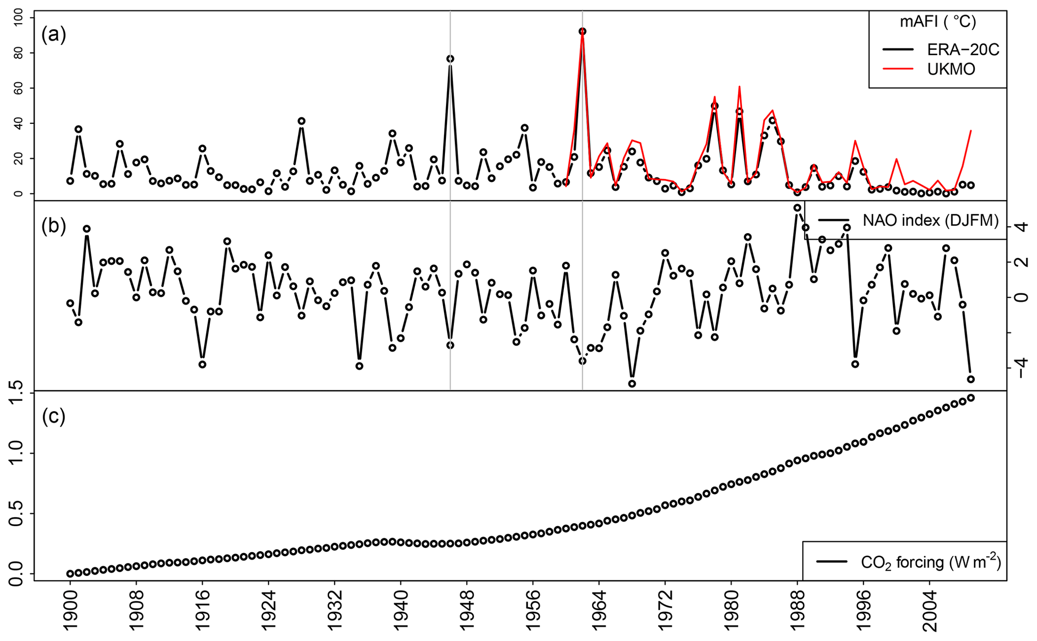
Figure 1Interannual variation of (a) the average AFI over UK (mAFI), (b) the North Atlantic Oscillation index (NAOI), and (c) CO2 forcing during the study period.
2.3 Anthropogenic forcing
Increases in concentration of greenhouse gases, such as carbon dioxide (CO2), are accompanied by increased radiative forcing, i.e. the difference between the incoming radiation from the sun and the outgoing radiation emitted from the Earth. This forcing arises from the ability of the gases to absorb long-wave radiation, thus reducing the amount of heat energy being lost to space and increasing the warming of the Earth's surface. Here we use the change in radiative forcing from CO2 as a predictor for climate change. It is calculated using the simplified expression (Myhre et al., 1998):
where is the radiative forcing change (in W m−2), Ci is the concentration of atmospheric CO2 at year i, and C1900 is the reference “pre-industrial” CO2 concentration at year 1900. Consequently, a doubling of CO2 corresponds to a change in the radiative forcing of 3.7 W m−2. Historical observations of global mean CO2 concentrations (in parts per million or ppm) are taken from Hansen et al. (2007). The temporal change in the CO2 radiative forcing during the 20th century is shown in Fig. 1c. Projections of future CO2 emissions are based on the Representative Concentration Pathway (RCP) scenarios adopted by the Intergovernmental Panel on Climate Change (IPCC) for its Fifth Assessment Report (AR5) (Collins et al., 2013).
3.1 Air Freezing Index and historical events
The daily temperature data are used to compute the AFI at each grid cell as the sum of the absolute average daily temperatures of all days with temperatures below 0 ∘C during the freezing period (Eq. 2). The freezing period in this study is defined from 1 June of a year to 31 May the following year, in order to include the entire winter season. Because AFI accounts both for the magnitude and duration of the freezing period, it is commonly used for determining the freezing severity of the winter season (Frauenfeld et al., 2007; Bilotta et al., 2015).
where AFIi is the AFI at cell i, N is the number of days in a winter season, and Td is the daily average temperature for a day d.
Maps of AFI values from ERA-20C for the severe winters of 1946/47, 1962/63, and 2009/10 are shown in Fig. 2. The winter of 1946/47 (i.e. season starting from 1 June 1946 to 31 May 1947) was a harsh European winter noted for its impact in the United Kingdom. It was notable for a succession of snowstorms from late January until mid-March, mainly associated with easterly airstreams (Booth, 2007). The mean AFI value (mAFI) in the entire UK (i.e. average of AFI values across all grid cells) mounted up to 75.6 ∘C, the second largest value during the analysed period.
Based on the AFI, the 1962/1963 winter season was the most severe winter in the 20th century and one of the coldest on record in the United Kingdom (Walsh et al., 2001). The “Big Freeze of 1962/63”, as it is also known, began on the 26 December 1962 with heavy snowfall and went on for nearly 3 months until March 1963. The cause of the cold conditions was the development of a large “blocking” anticyclone over Scandinavia and north-western Russia. Easterly winds on the southern edge of this system transported cold continental air westwards, displacing the more usual mild westerly influence from the Atlantic Ocean on the British Isles. Over the Christmas period, the Scandinavian High collapsed, but a new one formed near Iceland, bringing northerly winds. The mAFI in the entire UK (i.e. average of AFI values across all grid cells) mounted up to 90.9 ∘C, which is 6 standard deviations larger than the average of the entire 110-year period (14.0 ∘C). The event affected the southern part of the country more, as shown in Fig. 2.
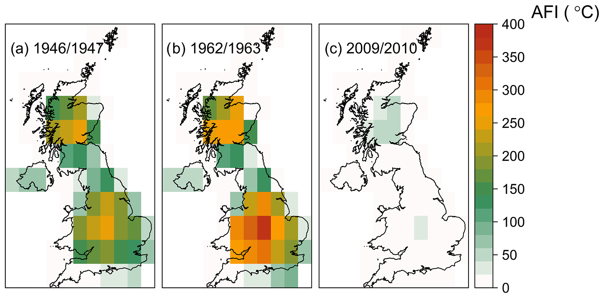
Figure 2Map of AFI values (in ∘C) for the winter seasons of (a) 1946/47, (b) 1962/63, and (c) 2009/10.
After 1962/63, a long run of mild winters followed until late 1978 and early 1979. However, temperatures in 1978/79 were not as low and the cold weather was interrupted frequently by brief periods of thaw (Cawthorne and Marchant, 1980). The mAFI value of winter 1978/79 reached 49.2 ∘C. The 1980s stands out as a decade with several cold spells in the UK, with mAFI values above 30 ∘C for the winters 1981/82, 1984/85, and 1985/86 (46.1, 32.6, and 41.0 ∘C, respectively).
For the last 10 years of our study period (from 2000 to 2010), the mAFI seems to be underestimated in the reanalysis data set (Fig. 1a). In particular, the winter of 2009/2010, which is well known to have brought frigid temperatures to the UK (Guirguis et al., 2011; Osborn, 2011; Seager et al., 2010; Prior and Kendon, 2011), has a mAFI value of only 4.7 ∘C (Fig. 2c), which is much lower than the long-term average (13 ∘C) and over 10 times lower than the mAFI value according to the UKMO data set (59.1 ∘C). No clear reason is known for this bias, but it might be related to possible spurious long-term trends in the atmospheric circulation (Bloomfield et al., 2018).
As shown in Fig. 1a, the two most severe winters in the century (1946/47 and 1962/63) were associated with a negative NAO phase (Murray, 1966; Osborn, 2011). As mentioned earlier, the NAO has a profound effect on winter climate variability in the Atlantic basin, accounting for more than half of the year-to-year variability in winter surface temperature over the UK (Scaife et al., 2005; Scaife and Knight, 2008). Not surprisingly, the ERA-20C mAFI over the entire UK is found to be significantly anti-correlated (, p value ) with NAOI. A negative correlation is found between the mAFI and forcing, but it is much less significant (, p value =0.08). Both NAO and climate change effects are included in the statistical model as predictors in order to account for their relation to cold winter spells in the UK as discussed in the following section.
3.2 Extreme value analysis
3.2.1 Stationary model
Since the historical data only extend for 110 years and our interest lies in very rare events (such as 1-in 200-year events), it is necessary to extrapolate by fitting an extreme value distribution. The generalized extreme value (GEV) family of distributions has been chosen, which includes the Gumbel, the Fréchet, and Weibull distributions. An additional term was included, the probability of no hazard (P0), in order to account for the cells, mainly on the south England coast, that have years with no negative temperatures at all. The probability therefore that the AFI value (X) inside a cell j is lower than or equal to a certain value (x) takes the form
where μ, σ, and ξ represent the location, scale, and shape parameters of the distribution, respectively. F(x) is defined when , μ∈ℜ, σ>0, and ξ∈ℜ. Its derivative, the GEV probability density function f(x), is given by
There are various methods of parameter estimation for fitting the GEV distribution, such as least squares estimation, maximum likelihood estimation (MLE), and probability weighted moments. Traditional parameter estimation techniques give equal weight to every observation in the data set. However, the focus in catastrophe modelling is mainly on the extreme outcomes, and, thus, it is preferable to give more weight to the long return periods. The tail-weighted maximum likelihood estimation (TWMLE) method developed by Kemp (2016) is employed here in order to estimate the GEV parameters. This method introduces ranking depended weights (w(r)) in the maximum likelihood. The weights are defined for each cell based on the historical winter season AFI values; i.e. the lowest historical AFI value in the cell (rank r=1 out of n observations) has the lowest weight, while the largest historical AFI value (rank r=n) has the largest weight, as follows:
Along with the TWMLE method described above, a second modification has been implemented in order to geographically smooth the GEV parameters. The smoothing is incorporated into the fitting process by minimizing the local (ranked) log-likelihood. More precisely, the log-likelihood at each grid cell i is calculated using all grid points but weighted by their distance:
where , dij is the distance between cell i and j, L is the smoothing parameter, and LogLj is the ranked log-likelihood for cell j.
The smoothing increases the sample size at each grid point, which thus leads to a more precise estimation of the parameters, especially for the shape parameter which is highly influential in estimating the hazard levels at high return periods. Because the data grid resolution is already coarse, a small length-scale parameter L of 20 km has been used (in comparison to the grid size).
Finally, in order to avoid an overestimate of the positive value of the shape parameter due to the small sample size (Lee et al., 2017), a modification of the maximum likelihood estimator using a penalty function is also applied for fitting the GEV. The penalty function penalizes estimates of ξ that are close to or greater than 1, following Coles and Dixon (1999).
Estimates of P0 for each grid cell are obtained by fitting a logistic regression model with intercept only (Eq. 7). As before, the fitting is performed against all grid cells, weighted by their distance dij, and a length scale of 20 km has been used. The model is extended in the non-stationary model to include covariates as described in Sect. 3.2.2.
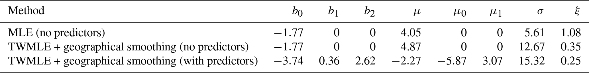
As an example, the GEV fit for a single cell over London is shown in Fig. 3. The curve fitted as described above (black line) is closer to the empirical estimates (black circles, computed as described in Sect. 4.1) in comparison with the GEV fit with no weighting applied (grey line). As shown in Table 1, for both fits the shape parameter is positive (i.e. both fits correspond to the Fréchet distribution), but for the approach followed here (TWMLE + geographical smoothing), the shape parameter is smaller, leading to a shorter tail and a curve that is nearer to the empirical estimate.
Maps of the fitted parameters are shown in Fig. 4. The probability of non-negative temperatures during a season (P0) is, as expected, larger around the coast, which has milder and less variable climate due to the water influence. This also explains the lower mean (location parameter) and larger spread (scale parameter) in the AFI distributions in the coastal regions in comparison to inland. The shape parameter, which affects the skew of the distribution, shows larger values in the southern part of the UK in comparison to the north, suggesting a less rapid increase in the maximum AFI estimates.

Figure 3AFI return period curves for a single cell over London: empirical fit (black circles), GEV fitted with MLE (grey line), and GEV fitted with TWMLE and geographical smoothing (black line).

Figure 4Maps showing the spatial distribution of the model fitted parameters: (a) P0 calculated as , (b) location μ, (c) scale σ, and (d) shape ξ.
3.2.2 Non-stationary model
In stationary models, the distribution parameter space is assumed to be constant for the period under consideration. However, such an assumption is not valid in the presence of atmospheric circulation patterns or anthropogenic changes. Regression approaches are often used to assess the influence of climatic factors on hazards and covariates such as global mean temperature, and CO2 concentration, and indexes of natural variability (such as NAOI) have been employed by several studies (Edwards and Challenor, 2013). In this study, a generalized linear model is introduced into the statistical distribution parameter estimates in order to improve the non-stationarity representation of the model. The NAOI and the global CO2 radiative forcing are chosen as covariates. There are some important caveats to this choice. First, other natural factors apart from NAO are not accounted for, and hidden co-varying effects might also be present. Also, while CO2 radiative forcing is linearly related to the equilibrium surface temperature, the relationship to transient surface temperatures further depends on the efficacy of ocean heat uptake (Winton et al., 2010). Both can lead to non-linear responses of the local UK climate, especially when extrapolating far in the future.
Despite the caveats, CO2 radiative forcing and NAO have some important advantages. First, both are accurately measured. Although a model that relies on global mean surface temperature may not have as strong correlations as the casual link is more indirect, it has the advantage that it does not rely on subtle regional patterns that are difficult to capture. They also provide a reasonable way to isolate the human and natural influences on extreme temperatures (see, for example, Risser and Wehner, 2017). While it would be possible to use a more locally defined metric (such as the change in the mean UK temperature, for example), this would include more unforced naturally occurring internal variability of the climate system, making it difficult to identify the changes that are driven by anthropogenic CO2 emissions. Finally, using a covariate such as the change in CO2 forcing avoids the difficulty with determining the start of the trend, and also results can be easily rescaled to a different time period or emission scenario, which is helpful for mitigation strategies.
The influence of NAO and of global warming is examined by exploring improvements to the distribution fits, after incorporating linear covariates on the distribution parameters, as follows:
-
-
,
where (b0, μ0) are the stationary model parameter estimates and (b1, μ1) and (b2, μ2) are linear transformations of the covariates NAOI and with respect to time, respectively.
Only non-stationarity with respect to P0 and the location parameter, μ, is discussed, since modelling temporal changes in σ and ξ reliably requires long-term observations in order to be estimated accurately (Katz et al., 2002; Cheng et al., 2014). In addition, a simple linear model is selected, as this is usually preferred when searching for trends in the occurrence of extreme events (Beguería et al., 2011). Finally, even though some climate modelling studies predict changes in the nature of NAO variability in an increasing CO2 climate (Rind et al., 2005; Woollings et al., 2010), the model does not include any interaction terms, as they have been found to be non-significant.
As before, the parameters of each cell are estimated, taking also into account its neighbouring cells weighted by their distance. The most pertinent model is selected, for each cell, using the χ2 test, based on the change in deviance, between the null-, one-, or two-predictor model. If the significance value is less than 0.01, the model is estimated to have a significant improvement over the reduced model. A separate test is performed for the P0 and the GEV model. As an example, in the case of the London cell, the model with two predictors for both P0 and the location parameter has been chosen (Table 1).
The spatial distribution of the parameters of the final model is shown in Fig. 5. Increasing NAOI or is consistent with a warming trend, leading to positive values of the P0 parameters (indicating increases in the number of years with no negative temperatures) and to negative values in the location parameters (indicating lower means in the AFI distributions). The NAO is found to affect more cells in total (90 %) in comparison to anthropogenic climate change (51 %). Notice, however, that due to the internal variability of the NAO, any signal from a climate change trend can be hidden in the limited observational period.
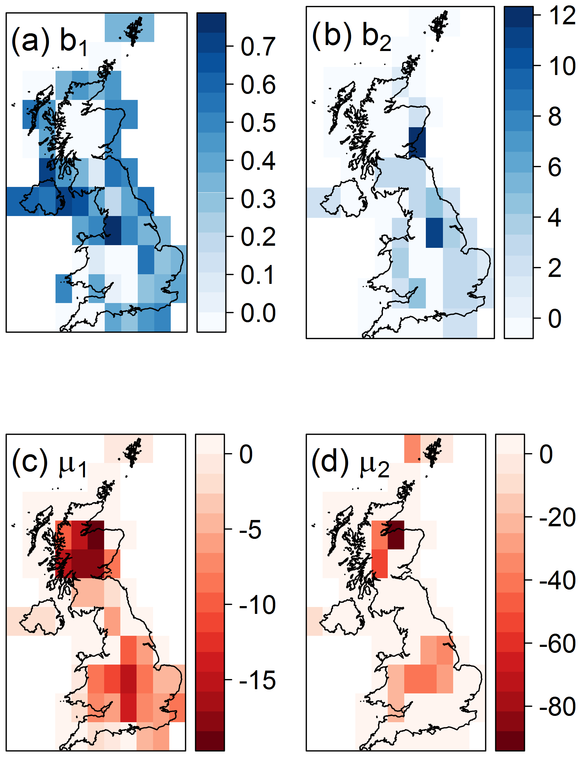
Figure 5Maps showing the spatial distribution of the non-stationary model parameters: (a) b1, (b) b2, (c) μ1, and (d) μ2. Zero values indicate linear trends not significant at the 0.01 level.
3.3 Vine copula model
The stochastic behaviour of the hazard (i.e. the AFI) at each cell is fully described by its corresponding GEV probability distribution, as described in Sect. 3.2. However, insurance portfolio loss analysis requires the calculation of the combined stochastic behaviour of the hazard across all the model domain (i.e. all cells). This is described by the joint distribution of the hazard, which, according to Sklar's theorem, can be fully specified by the separate marginal GEV distributions and by their copula, which models the hazard dependence between the cells. Vine copulas provide a flexible solution to this problem based on a pairwise decomposition of a multivariate model into bivariate (conditional and unconditional) copulas, whereby each pair-copula can be chosen independently from the others. A brief introduction to the vine copula methodology can be found in Appendix A.
In this study, the joint multivariate hazard distribution of the AFI across all the model domain (67 cells) is decomposed as a product of marginal and pair-copula probability density functions (pdfs). The pair-copulas are fitted using the R (https://www.r-project.org/, last access: 12 March 2019) package VineCopula (Schepsmeier et al., 2017; Brechmann and Schepsmeier, 2013). The method follows an automatic strategy of jointly searching for an appropriate R-vine (regular vine) tree structure and its pair-copula families and estimating their parameters developed by Dißmann et al. (2013). This algorithm selects the tree structure by maximizing the empirical Kendall's τ values, based on the premise that variable pairs with high dependence should contribute significantly to the model fit and should be included in the first trees.
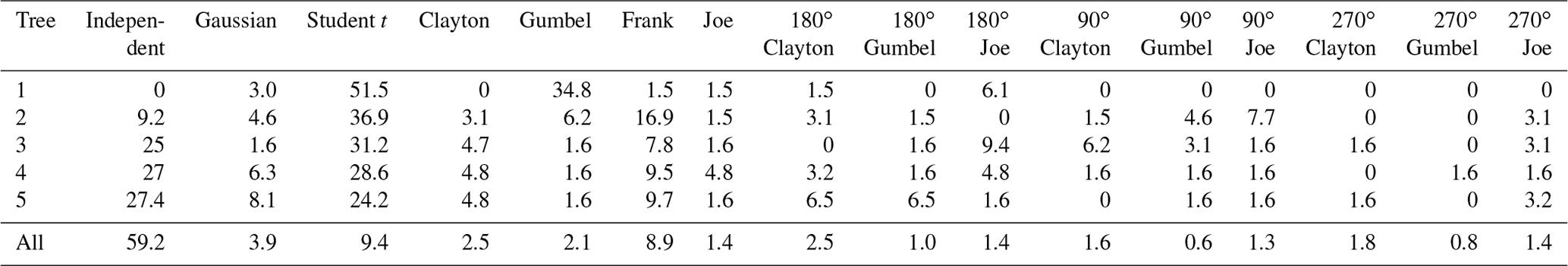
Table 2Percentage of family types used for the first five trees of the R-vine model.
The copula family types for each selected pair in the first tree are determined using the Akaike information criterion (Brechmann and Schepsmeier, 2013). For computational reasons, the two-parameter Archimedean copulas are excluded from this analysis, which, however, only has a negligible impact on the results (not shown). The copula parameters are estimated sequentially (using maximum likelihood estimation) from the top tree until the last tree, as described in Czado et al. (2013). This approach only involves estimation of bivariate copulas and has been chosen since it is computationally much less demanding than the joint maximum likelihood estimation of all parameters at once.
The percentage of family types used for the first few trees of the selected R-vine model (RVM) is shown in Table 2. The large majority of the pairs in all trees are estimated to be independent (59 %), but these pairs mainly occur at the higher trees, since the most important dependencies are captured in the first trees (Brechmann and Schepsmeier, 2013; Dißmann et al., 2013). Large dependencies, with Kendall's τ coefficients greater than 0.90, are found as expected between neighbouring cells but remain important across the whole model domain due to the nature of the hazard: the AFI assesses the freezing temperatures during the entire winter and, thus, is less associated with small-scale local phenomena that can cause important spatial variation. At the first tree, 52 % of the selected bivariate copulas are found to belong to the Student t copula and 35 % to the Gumbel family, which exhibit positive dependence in the tails. Gumbel, in particular, has a greater dependence in the positive tail than in the negative and thus implies greater dependence at larger AFI values than at lower ones. From the third tree onwards, the percentage of independent families is always larger than 40 %.
The small sample size used (110 years of data) in conjunction with the high dimensions of the modelled pdf (67) is of concern in this study since this can lead to large uncertainties in the resulting pdf, which can also propagate in the estimated return periods. The impact of the short sample size on the uncertainties in the results is quantified using a bootstrap technique, as described in Sect. 3.4.
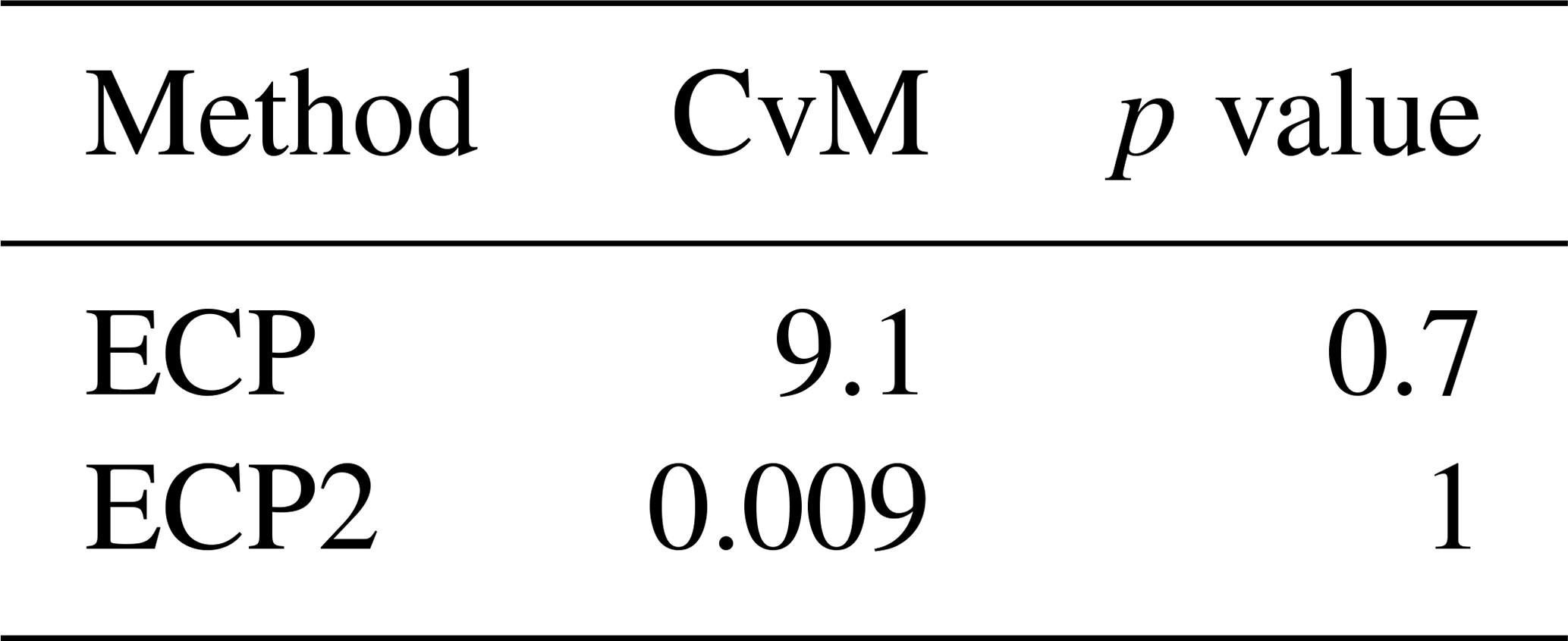
Goodness of fit (GOF) is calculated using the Cramér–von Mises test, which compares the final selected RVM with the empirical copula. The RVineGofTest algorithm of the same R package implements different methods to compute the test, which, however, usually perform poorly in cases of small sample sizes and at higher dimensions as is the case for this work (Schepsmeier, 2013). Nevertheless, Table 3 shows the GOF results for two of these methods. The p value is found to be larger than 0.05, which is an indication that the fitted RVM cannot be rejected at a 5 % significance level. However, given also the quite large p values, a type II error cannot be excluded. Nevertheless, the suitability of the model, in comparison to the empirical data, is further discussed in the Results section as well.
Table 3Goodness-of-fit values for the Cramér–von Mises (CvM) statistic based on the empirical copula process (ECP) and based on the combination of the probability integral transform and empirical copula process (ECP2) as implemented in the VineCopula R package.
In the case of the stationary model, the vine copula is employed to model the entire spatial dependence of the AFI in the UK. On the other hand, the spatial AFI structure in the case of the non-stationary model is modelled in two ways: (a) by quantifying the dependence on NAO or CO2 in each location, treating each location as conditionally independent, and then inducing spatial dependence through the variation of NAO or CO2 and (b) by fitting the RVM to all the residual dependencies associated with the AFI between the cells; these account for dependencies between cells resulting from other large-scale circulation patterns and also regional climate variability (e.g. due to effects of local orography, land–sea contrast, and small-scale atmospheric features such as convective cells). Notice, however, that the effect of NAO or CO2 on the residual hazard dependency structure is not taken into account here. Recently, a methodology that offers the possibility to include such meteorological predictors in a vine copula model has been developed by Bevacqua et al. (2017) and Bevacqua (2017) and is something to be addressed in a future study.
3.4 Stochastic simulation and uncertainty estimation via parametric bootstrap
The pdf is used to simulate 100 000 years of winter seasons in the UK. For each year, the simulated AFI values at each grid cell depend on the other cells based on the fitted RVM. Long simulations are needed to obtain numerically converged results, i.e. convergence to the “true” return period. Our focus here is the 200-year RP, which is commonly associated with capital and regulatory requirements. By repeating the simulation several times, it has been assessed that 100 000 years of winter seasons is long enough to neglect the Monte Carlo uncertainty. The stationary model is used to generate a stochastic set which corresponds to the current hazard experience. The non-stationary model permits us to create additional stochastic sets that represent different climate conditions. In order to assess the influence of climate change on UK cold spells, three separate stochastic sets, of 100 000 years each, have been created as follows:
-
pre-industrial climate ( W m−2), corresponding to the pre-industrial (1900) concentration of CO2 (296 ppm);
-
current climate ( W m−2), corresponding to a present-day (2018) concentration of CO2 (400 ppm);
-
future climate ( W m−2), corresponding to the future year 2030 concentration of CO2 (435 ppm), according to the RCP4.5 emission scenario.
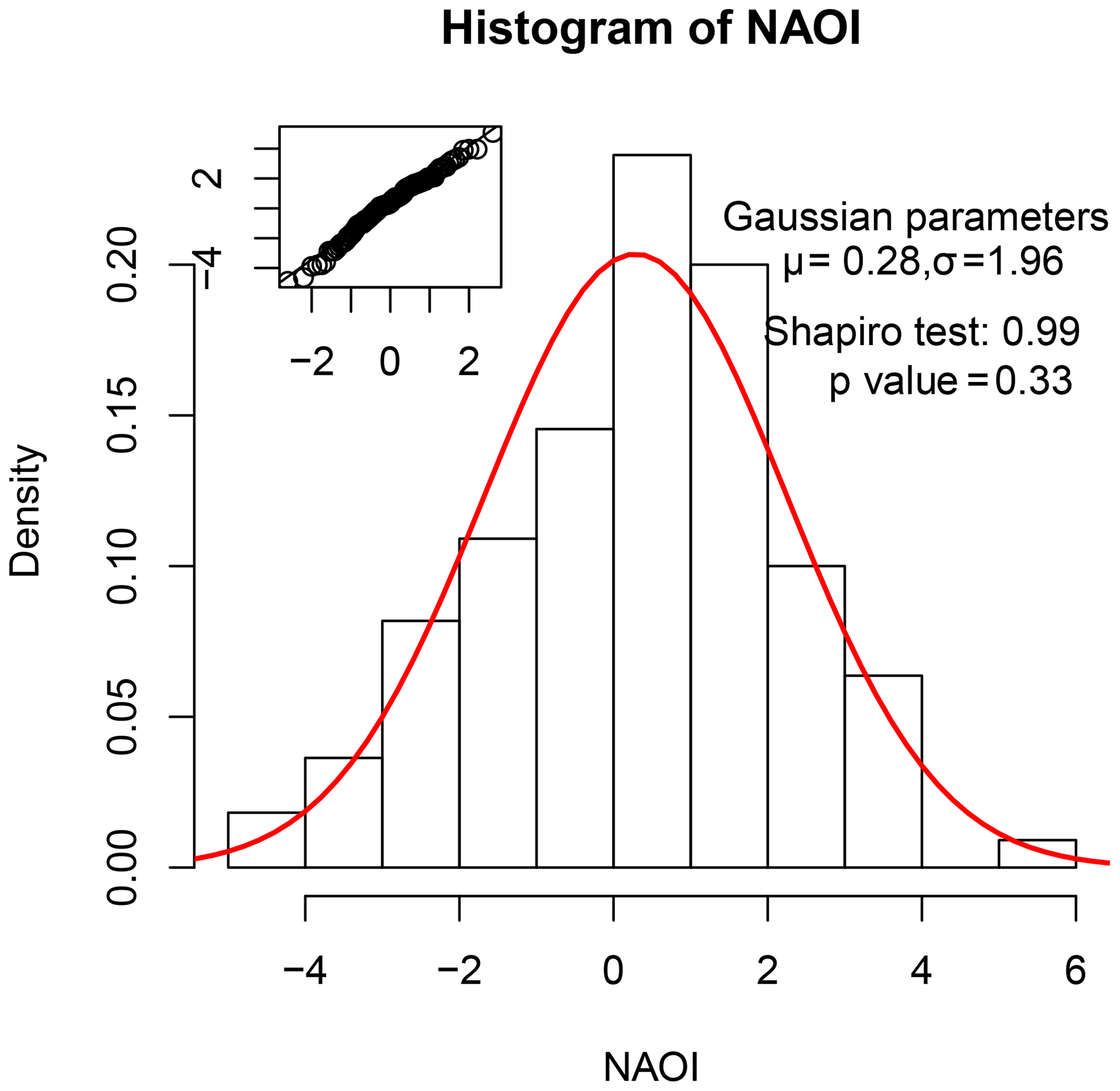
The choice of the year 2030 assures a relative close time distance which is more relevant for the insurance industry (UNEP, 2015). At the same time, extrapolating far in the future is particularly problematic, since it relies on the assumption of the stability of these linear relationships, even though they may be significantly altered by changing boundary conditions. The change in the CO2 radiative forcing is calculated here based on the RPC4.5 scenario (2 W m−2), but similar values are projected for 2030 by the other RCP scenarios as well (Meinshausen et al., 2011). Each year of the three stochastic sets above is associated with a random NAOI value that has been simulated assuming a Gaussian distribution, fitted to the historical NAOI data set (see Fig. 6). The influence of NAO on each one of these sets can thus be discerned by selecting only the simulated years with negative or positive NAOI values.
The small sample size used in this study (110 years of data) together with the high dimensions of the modelled pdf (67) can lead to large uncertainties in the estimated return periods. Following Bevacqua et al. (2017), the model uncertainty is assessed using a parametric bootstrap approach, for which a large number of models are created using, instead of observations, randomly simulated data from the selected RVM as a basis. In particular, confidence intervals are constructed as follows:
-
A simulation with the same length as the observed data (i.e. 110 years) is repeated for B=500 times.
-
For each of these B=500 samples, a new full model is fitted (including new GEV and logistic regression model parameters at each cell and new RVM structure, pair-copula families and parameters) following the methodology described in Sect. 3.3.
-
For each of the resulting B=500 RVMs, a simulation of 10K years of winter seasons is performed. The uniform variables are then transformed using the (new) inverse marginal pdfs, and the corresponding return period levels are estimated.
-
The uncertainty in the return levels is estimated by identifying the 95 % confidence interval (i.e. the range 2.5 %–97.5 %) from these 500 return level curves.
Due to computational constraints, confidence intervals are only computed for the stationary model. In addition, the simulation length has been reduced to 10 000 years (instead of 100 000), which implies that part of the calculated uncertainty is due to Monte Carlo sampling variability. In order to investigate the sources of this uncertainty further, the uncertainty associated with the RVM is only separated from the uncertainty of the full model, i.e. of the joint pdf, by calculating confidence intervals with the same approach as described above but using the same marginal pdfs in each bootstrap repetition.
4.1 Return period maps
The obtained stochastic sets (see Sect. 3.4) are used to create return period maps for the different climatic conditions. Figure 7a, b, and c represent the AFI values that occur once every 10, 25, and 50 years based on the stationary model. The empirical return periods are also plotted for comparison (Fig. 7d, e, and f). These are calculated for each cell as , where P represents the cumulative probabilities of the ranked values and is calculated based on the Weibull formula (Makkonen, 2006). The spatial pattern is consistent between the empirical and stochastic sets, showing the largest AFI values in high elevation areas, as expected. However, the empirical values are in general somewhat larger than the stochastic set. This difference is driven by the exceptional 1962/63 event, which is estimated empirically at 1 in 110 years but is predicted to be less frequent according to the GEV fits. The probability of such an event happening today is discussed in detail in Sect. 4.2.2.
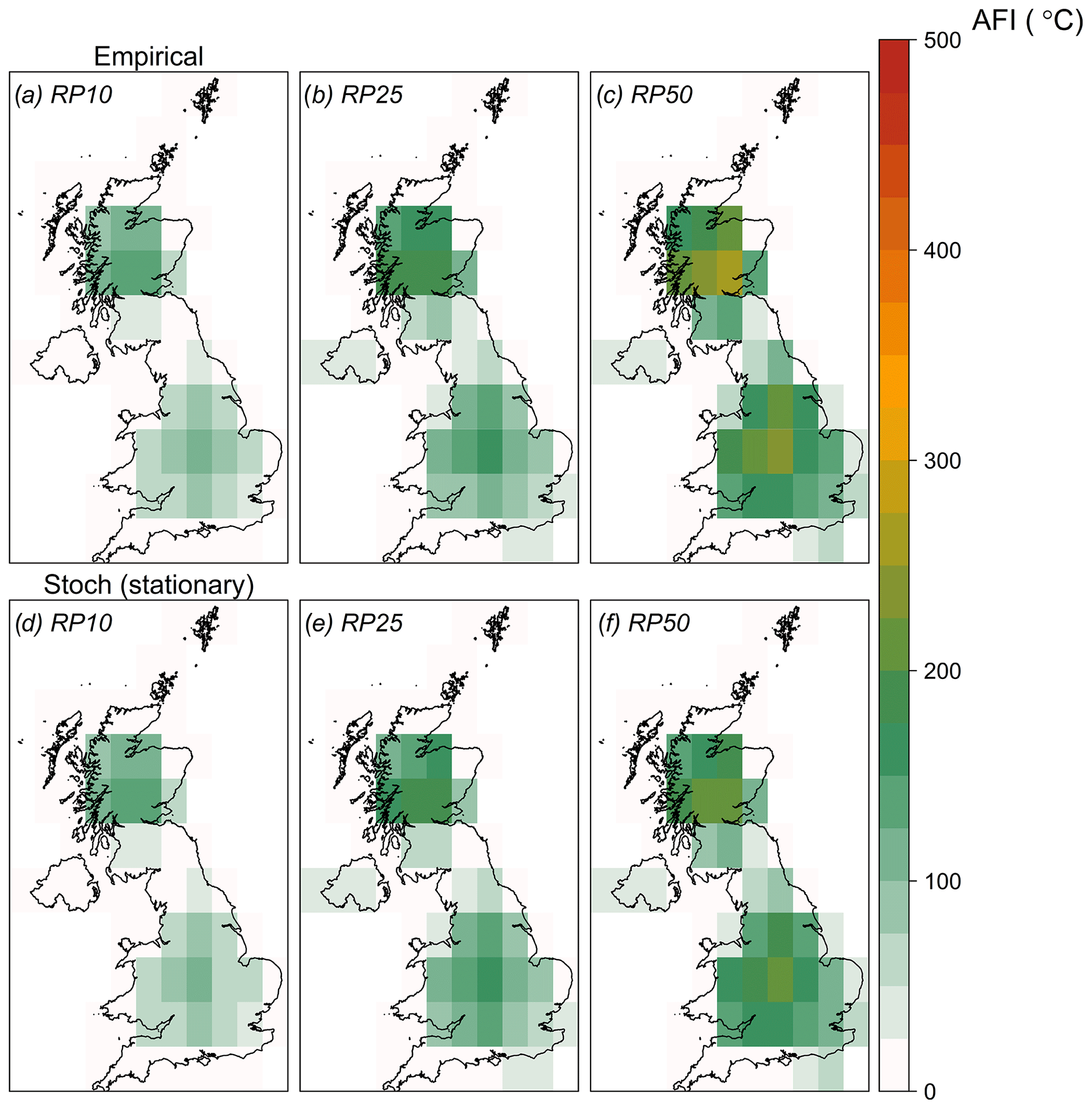
Figure 7(a–c) Maps of stochastic AFI values (in ∘C) for return periods of (a) 10, (b) 25, and (c) 50 years. (d–f) Maps of the corresponding empirical AFI values.
Return period maps at higher return periods (100, 200, and 500 years) for the pre-industrial, current, and future climate stochastic sets are shown in Fig. 8. In the beginning of the 20th century, the UK was experiencing much colder winters than today. By 2030, the future climate change scenario, extreme cold events with an AFI larger than 100 ∘C become quite rare (above a 100-year RP) everywhere, except in mountainous regions. At high return periods and across all scenarios, the model predicts larger AFI values for the southern part of the UK in comparison to the north. The extreme AFI values in the south are driven by the exceptional 1962/63 winter which has been more severe in the south than the north (see Fig. 2b). Excluding this winter from the analysis results in much lower AFI values in most of the region (not shown).
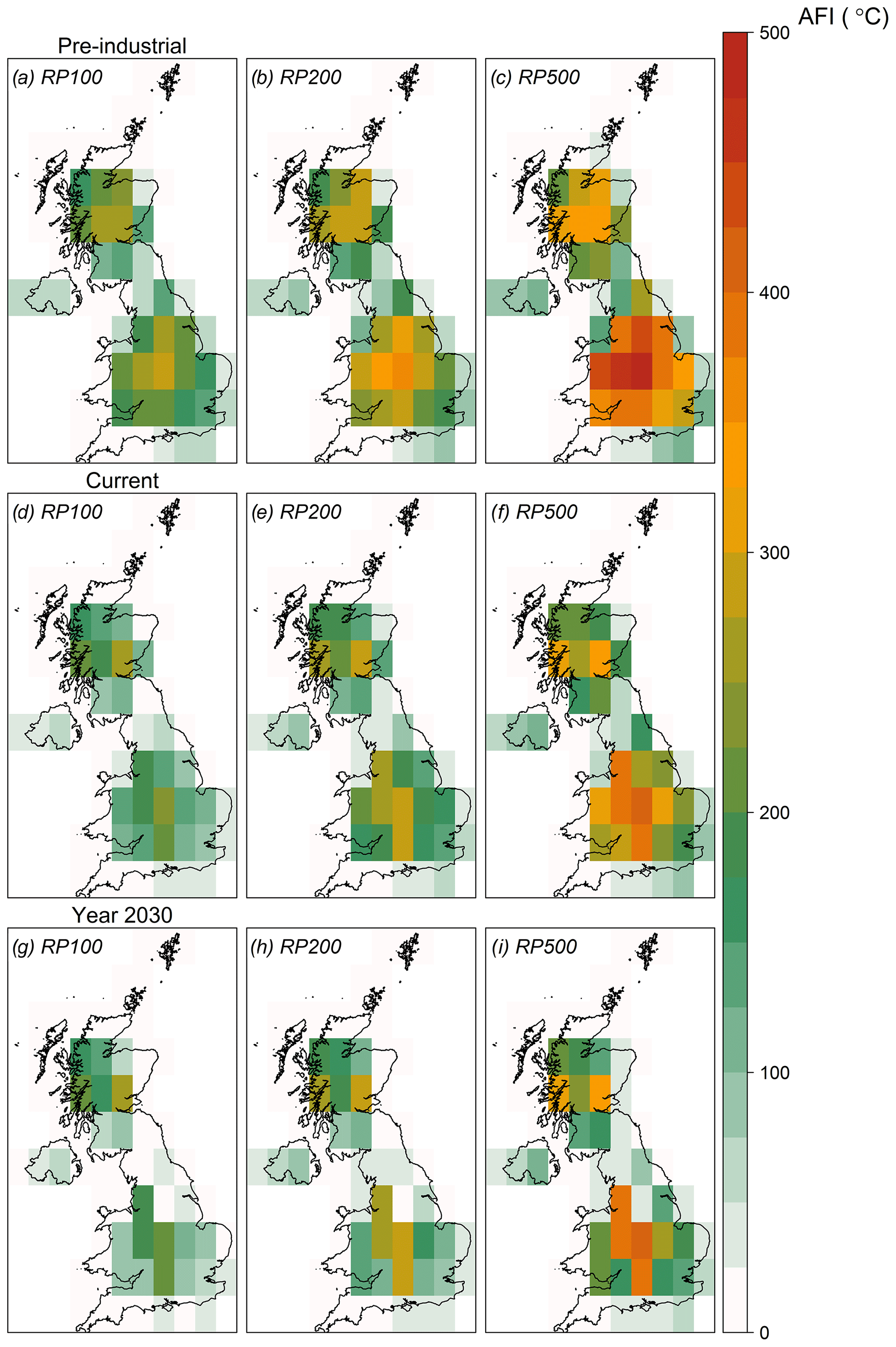
Figure 8Maps of stochastic AFI values (in ∘C) for return periods of 100, 200, and 500 years for pre-industrial (a–c), current (d–f), and future (g–i) climate.
4.2 Regional return period AFI curves
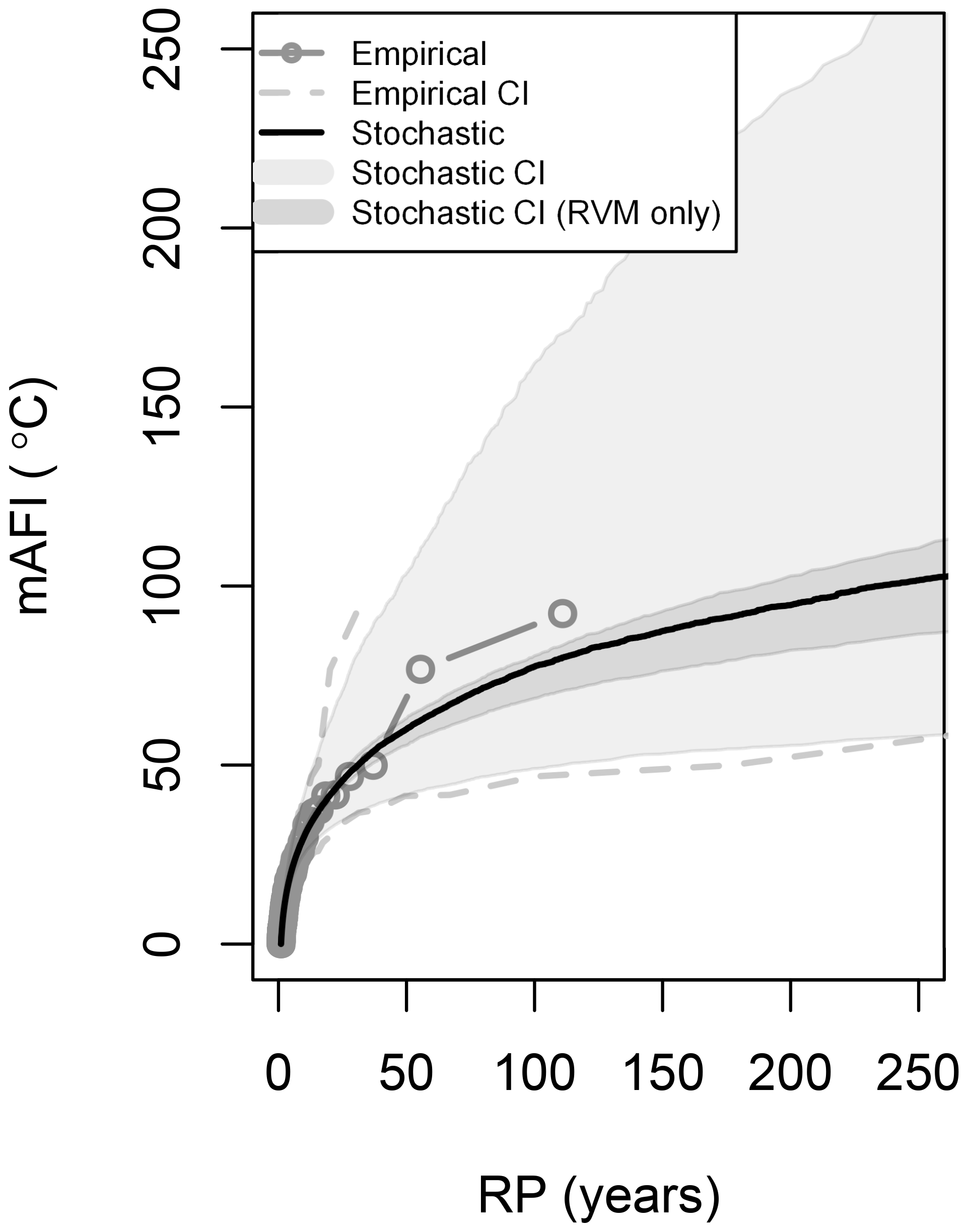
The vine copula methodology permits the estimation of the hazard return periods over aggregated regions in the UK. Since our focus is mainly on inhabited areas, for each simulation year (y) and for each region, the weighted AFI (wAFI) is computed, whereby the AFI value at each cell j is weighted by the corresponding number of residential properties (nj), as shown in Eq. (8). The weighted AFI thus places more weight on the hazard over large populated urban areas than agricultural or mountainous areas. The number of residential properties in the UK is taken from the PERILS Industry Exposure Database (https://www.perils.org/, last access: 12 March 2019), which contains up-to-date high quality insurance market data at CRESTA level (Catastrophe Risk Evaluating and Standardizing Target Accumulations; https://www.cresta.org/, last access: 12 March 2019) based on data directly collected from insurance companies writing property business in the UK. Return period wAFI curves for both the empirical and the stochastic data are shown in Fig. 9. An analogous return period plot based on the mAFI, i.e. without weighting, can be found in the Appendix (Fig. A1).
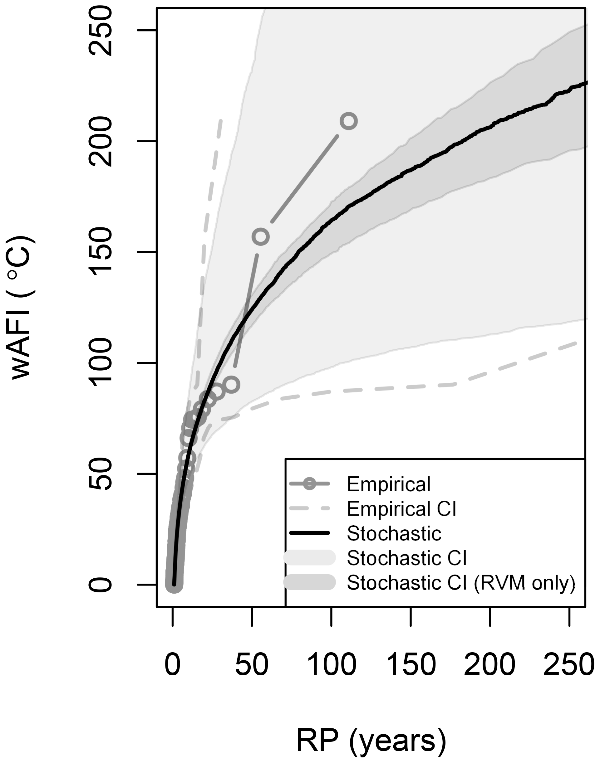
Figure 9Return period curves of the wAFI (in ∘C) based on the historical data (grey) and the stochastic model (black). The 95 % confidence intervals are shown as dashed grey lines for the historical data and as a shaded grey area for the stochastic model. The dark shaded area represents the stochastic uncertainty due to the RVM model alone.
4.2.1 Model uncertainty
The stationary model is utilized to analyse the uncertainty in the model results and investigate its sources. Figure 9 shows the empirical and the stochastic return period curves of the wAFI for the entire UK, together with their associated uncertainties. The empirical return periods calculation is described in Sect. 4.1, while their uncertainty intervals are computed from the 2.5th and 97.5th quantile of the beta probability distribution function (Folland and Anderson, 2002). The stochastic curve and confidence intervals are computed as described in Sect. 3.4. The uncertainty in the model is found to be large, only marginally lower than the empirical estimates, and is associated with the short historical record length. Most of the uncertainty (around 90 % for RPs greater than 50 years) appears to originate from the uncertainty in the GEV distribution parameters, with the remaining 10 % being due to the RVM model (dark shaded area in Fig. 9). Extreme-value theory is considered as a state-of-the-art procedure to find values for return periods that amply exceed the record length and has been utilized in this study. However, a common difficulty with extremes is that, by definition, data are rare, and as a result, the shorter the record length, the more inaccurate the estimation of the GEV parameters is. The results presented in the following sections should therefore be interpreted with awareness of the existing uncertainties.
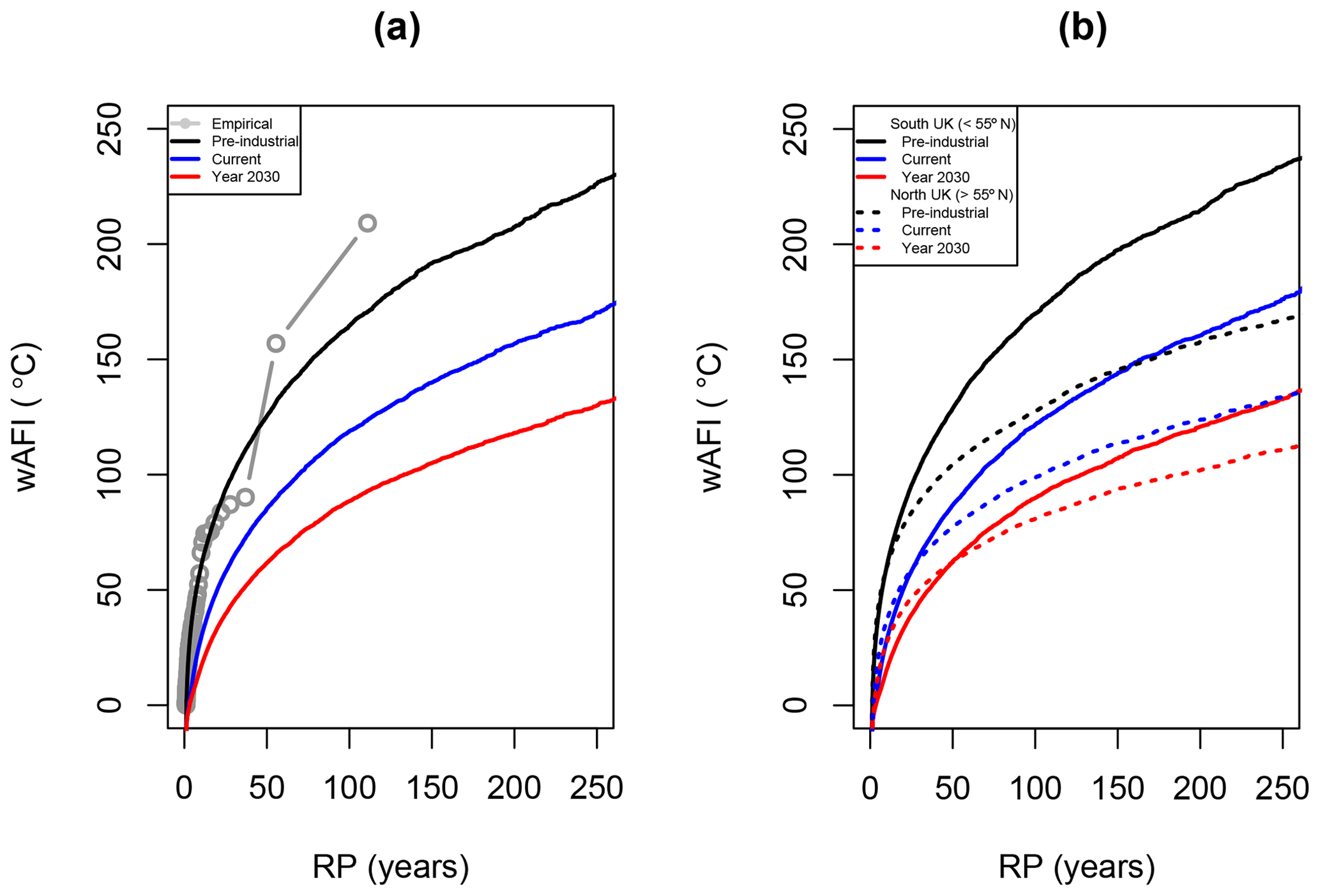
Figure 10(a) Return period curves of the wAFI (in ∘C) based on the historical data (grey) and the stochastic model for three different climate conditions: pre-industrial (black), current (blue), and future (red). (b) Same as panel (a) but separated between the south UK (full lines) and the north UK (dashed lines). Only stochastic sets are shown.
4.2.2 The 1962/63 winter return period and climate change influence
Return period curves for the stochastic sets under pre-industrial, current, and future climate conditions are shown in Fig. 10. The 1962/63 winter, with a wAFI of 209 ∘C, was the coldest in the reanalysis data in the UK, and, thus, it is estimated empirically as a 1- in 110-year event (i.e. the length of the data set). This corresponds well with the Central England Temperature record, the oldest continuously running temperature data set in the world (Manley, 1974). According to the latter, only two other winters (1683/84 and 1739/40) have been colder than 1962/63 in the last 350 years, suggesting a return period in the range of 110–120 years as well. The stationary model overestimates this winter's return period, which is estimated to be 205 years across the whole of the UK (Table 4). Especially in the south of the UK, the model suggests that this event was particularly unusual. In the northern part of the UK, on the other hand, the model suggests a lower return period of 106 years, closer to the empirical estimate.
The non-stationary model suggests that under current climate conditions, such an extreme event is approximately 2 times less likely to occur than in the 1960s. This agrees with Massey et al. (2012), who used climate model simulations to demonstrate that cold December temperatures in the UK are now half as likely as they were in the 1960s. Christidis and Stott (2012) also indicate that human influence has reduced the probability of such a severe winter in the UK by at least 20 % and possibly by as much as 4 times, with a best estimate that the probability has been halved. On the other hand, some recent studies have argued that warming in the Arctic could favour the occurrence of cold winter extremes and might have also been responsible for the unusually cold winters of 2009/10 and 2010/11 in the UK (Francis and Vavrus, 2012; Tang et al., 2013). This hypothesis though is still largely under debate; see, for example, Barnes and Screen (2015) and Wallace et al. (2014).
Table 4Return period estimates (in years) for the 1962/63 winter freeze event, based on wAFI.
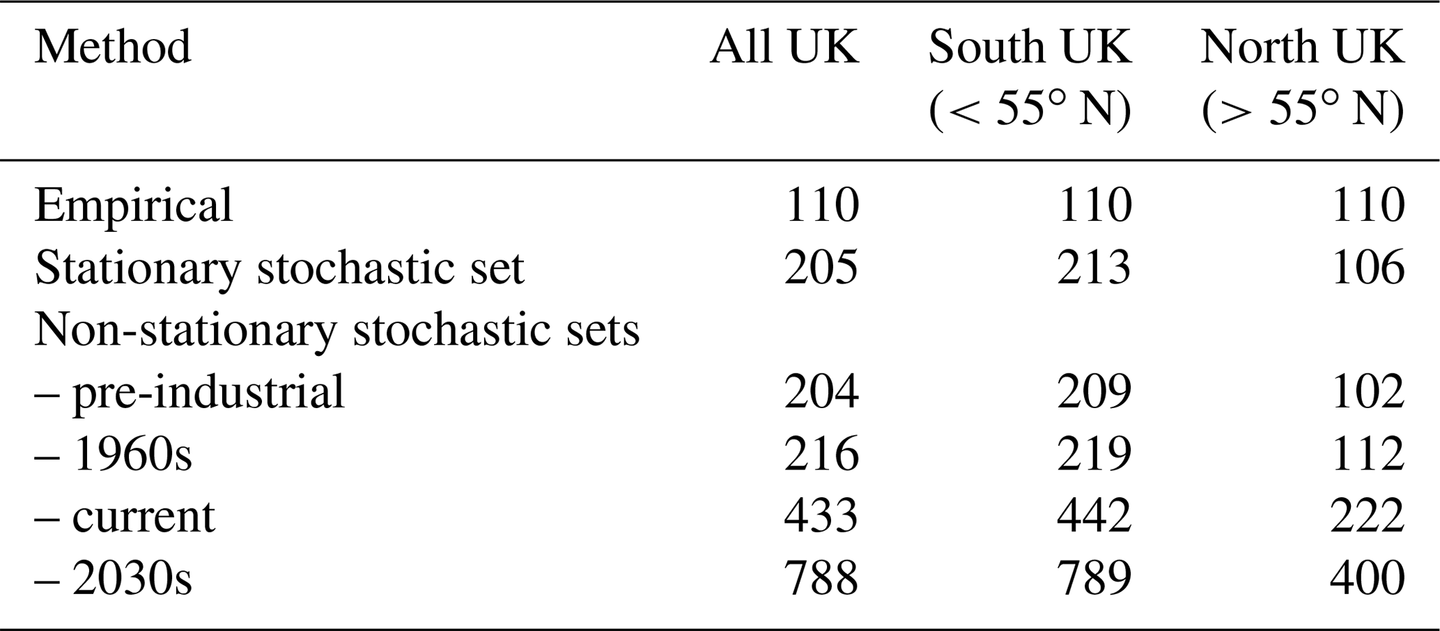
By the year 2030, an event of the same severity as 1962/63 is predicted to become almost 2 times less infrequent, with a return period of 788 years. Figure 10a shows an important reduction in the probability of occurrence of cold extreme events across the whole distribution as a result of the increase of anthropogenic CO2 concentrations. Larger reductions are found for the most extreme events as well, which is probably related to the large increase of the probability of no negative temperatures (P0) for several cells, especially around the coast (see Fig. 8). Similar results are found in both the northern and the southern part of the UK as well (Fig. 10b).
4.2.3 NAO influence
The profound effect of the NAO on the winter surface temperature over the UK has been reported by several studies (Scaife et al., 2005; Scaife and Knight, 2008; Osborn, 2011). In conjunction with these studies, the model predicts that a negative (positive) NAO phase increases (decreases) the probability of a cold event in the UK substantially. Figure 11 shows the RP curve of the current climate wAFI, along with RP curves computed solely from simulated years with NAOI values greater than 1 (i.e. representing the positive NAO phase) or years with NAOI values lower than 1 (i.e. representing the negative NAO phase). On average, extreme cold winters are estimated to be ≈3–4 times more likely to occur during the negative phase than the positive phase. As an example, an event with a wAFI of 100 ∘C has a return period of 39 years, assuming a negative phase, and 1 in 133 years, assuming a positive phase. Because of its intrinsic chaotic behaviour, the NAO is difficult (if possible at all) to predict (Kushnir et al., 2006). Nevertheless, numerical seasonal forecast systems are currently rapidly improving and have even shown some success in the past (Graham et al., 2006; Folland et al., 2006). Incorporating such information in models could be very useful from a catastrophe risk management perspective.

Figure 11Return period curves of the wAFI (in ∘C) based on the current climate stochastic model and assuming a variable NAOI as described in the text (black line). Return period curves based on negative (lower than −1) and positive (larger than 1) values of NAOI are shown by green and orange lines, respectively.
As already mentioned, the effect of the NAO or CO2 radiative forcing in the hazard dependency structure has not been taken into account here and is something to be addressed in a future study. Another point that requires further consideration is the mechanisms that control and affect the NAO and its temporal evolution and in particular how the NAO responds to external CO2 forcing (Hurrell, 2015).
This paper presents a probabilistic model of extreme cold winters in the United Kingdom. The hazard is modelled using the Air Freezing Index, an index which accounts for both the magnitude and the duration of air temperature below freezing and is calculated from the ERA-20C reanalysis temperature data covering the period from 1900 to 2010. Extreme value theory has been applied in order to estimate the probability of extreme cold winters spatially across the UK. More importantly, the spatial dependence between regions in the UK has been assessed through a novel approach which takes advantage of the vine copula methodology. This approach allows the modelling of concurrent high AFI values across the country, which is necessary in order to assess the extreme behaviour of freeze events reliably.
Recognizing the non-stationary nature of climate extremes, the model also incorporates the NAO and climate change effects as predictors. Stochastic sets of 100 000 years representing different climate conditions (i.e. pre-industrial, current, or future climate and positive or negative NAO) have been generated, and the return periods of extreme cold winters in the UK, such as the Big Freeze of 1962/63, have been estimated. According to the model, the occurrence of such an event is calculated to have decreased approximately 2 times during the course of the 20th century as a result of anthropogenic climate change. The model further predicts that by the 2030s, extreme cold winters will become even more uncommon and will occur about 2 times less frequently under the influence of increasing CO2 concentrations. The frequency of extreme cold spells in the UK has been found to be heavily modulated by the NAO as well. A cold event is estimated to be ≈3–4 times more likely to occur during the negative phase than the positive phase.
However, considerable uncertainty exists in these estimates, which should be interpreted with caution. The 110-year reanalysis record used in this study is estimated to be short, and the level of uncertainty in extremal estimates with long return periods is high. Additional uncertainty may also be introduced by possible spurious trends in the reanalysis data set. A longer record of temperature data would be necessary in order to reduce the uncertainty, and high-quality long-term reanalysis products with multiple ensemble members could help in this direction.
The ERA-20C data are available under a Creative Commons Attribution 4.0 International License at https://www.ecmwf.int/en/forecasts/datasets/reanalysis-datasets/era-20c (last access: 12 March 2019; Poli et al., 2016). The UK Met Office data are available under the Open Government Licence at https://www.metoffice.gov.uk/climate/uk/data/ukcp09 (last access: 12 March 2019; Perry et al., 2009). The Hurrell North Atlantic Oscillation Index (station based) dataset is freely available at https://climatedataguide.ucar.edu/climate-data/hurrell-north-atlantic-oscillation-nao-index-station-based (last access: 12 December 2016; Hurrell, 2003). Historical observations of global mean CO2 concentrations are freely available at https://data.giss.nasa.gov/modelforce/ghgases/Fig1A.ext.txt (last access: 12 March 2019; Hansen et al., 2007). The Perils Industry Exposure Database is available on an annual subscription basis (https://www.perils.org/products/industry-exposure-and-loss-database, last access: 12 March 2019). The perils data are used in this study to calculate the weighted AFI in Sect. 4.2. However, results without weighting do not alter the conclusions of this study and are also presented in the Appendix (Fig. A1).
According to Sklar's theorem, the joint multivariate distribution of a set of d random vectors can be fully specified by the separate marginal distributions and by their (d-dimensional) copula, which defines the dependence structure between them. More precisely, consider a vector of of random variables with a joint probability density function (pdf), . Sklar's theorem (Sklar, 1959) states that any multivariate continuous distribution function with marginals can be written as
for some appropriate d-dimensional copula C, which is uniquely determined on [0,1]d.
The probability density function (pdf) of X, , can be found by taking the partial derivatives with respect to X:
where is the copula density, given by
Expression (A2) is important in terms of modelling because it permits a multivariate density to be defined as the product of marginal pdfs and a copula density function that captures the dependence between the random variables (Abbara and Zevallos, 2014). For a theoretical introduction to copulas, see Nelsen (2006), Meucci (2011), Joe (2014), and Durante and Sempi (2015); for a practical engineering approach and guidelines, see Genest and Favre (2007), Salvadori and Michele (2007), and Salvadori et al. (2014, 2015).
To quantify the dependence between variables, different measures have been defined, addressing different aspects of dependence. A common measure of overall dependence is the Kendall rank correlation coefficient, commonly referred to as Kendall's τ coefficient (Genest and Favre, 2007). However, dependence of rare events cannot be measured by overall correlations: even if two variables are completely uncorrelated, there can be a significant probability of a concurrent extreme event in the two; i.e., they can still be tail-dependent. Tail dependence describes the amount of dependence in the lower tail or upper tail of a bivariate distribution. For its mathematical definition, see Haff et al. (2015).
One important complication is that identifying the appropriate d-dimensional copula is not an easy task. In high dimensions, the choice of adequate families is rather limited (Brechmann and Schepsmeier, 2013). Standard multivariate copulas either do not allow for tail dependence (i.e. multivariate Gaussian) or only have a single parameter to control tail dependence of all pairs of variables (Student t and Archimedean multivariate copulas). This is particularly problematic for catastrophe modelling applications, for which a flexible modelling of tails is vital to assess the extreme behaviour of natural events reliably.
Vine copulas provide a flexible solution to this problem based on a pairwise decomposition of a multivariate model into bivariate (conditional and unconditional) copulas, whereby each pair-copula can be chosen independently from the others. In particular, asymmetries and tail dependence can be taken into account as well as (conditional) independence to build more parsimonious models. Vines thus combine the advantages of multivariate copula modelling, that is the separation of marginal and dependence modelling, and the flexibility of bivariate copulas (Brechmann and Schepsmeier, 2013).
As an example, in a four-dimensional case, the joint pdf can be decomposed as a product of six pair-copulas (three unconditional and three conditional) and four marginal pdfs, as shown in Eq. (A4):
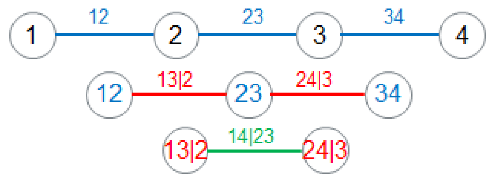
Figure A2Example of four-dimensional R-vine trees corresponding to the decomposition shown in Eq. (A4).
The above decomposition is not unique, and Bedford and Cooke (2002) introduced a graphical structure called regular vine (R-vine) structure to represent this decomposition with a set of nested trees. The dependence structure with three trees for the four-dimensional example above is shown in Fig. A2. More details on vine copulas can be found in Aas et al. (2006), Schirmacher and Schirmacher (2008), Czado (2010), and Schepsmeier (2013).
SK conceived the presented idea, performed the computations, discussed the results, and wrote the manuscript.
This research is sponsored by the author's employer, Guy Carpenter, and may lead to the development of products that may be licensed to Guy Carpenter clients.
The author would like to thank the editor and the two anonymous reviewers for
their comments, which helped to greatly improve the quality of this article.
I would like to thank my colleagues at Guy Carpenter for reviewing the
content and providing valuable feedback.
Edited by: Piero Lionello
Reviewed by: two anonymous referees
Aas, K., Czado, C., Frigessi, A., and Bakken, H.: Pair-copula constructions of multiple dependence,, Tech. rep., Munich University, Institute for Statistics, available at: https://epub.ub.uni-muenchen.de/1855/1/paper_487.pdf (last access: 12 March 2019), 2006. a
Abbara, O. and Zevallos, M.: Assessing stock market dependence and contagion, Quant. Financ., 14, 1627–1641, https://doi.org/10.1080/14697688.2013.859390, 2014. a
ABI: Industry Data Downloads, Tech. rep., Association of British Insurers, available at: https://www.abi.org.uk/data-and-resources/industry-data/free-industry-data-downloads/ (last access: 1 June 2018), 2017. a, b
AIR: About Catastrophe Models, Tech. rep., AIR Worldwide, available at: https://www.air-worldwide.com/Publications/Brochures/documents/About-Catastrophe-Models/ (last access: 12 March 2019), 2012. a
Barnes, E. A. and Screen, J. A.: The impact of Arctic warming on the midlatitude jet-stream: Can it? Has it? Will it?, WIRES Clim. Change, 6, 277–286, https://doi.org/10.1002/wcc.337, 2015. a
Bedford, T. and Cooke, R. M.: Vines – a new graphical model for dependent random variables, Ann. Stat., 30, 1031–1068, https://doi.org/10.1214/aos/1031689016, 2002. a
Beguería, S., Angulo-Martínez, M., Vicente-Serrano, S. M., López-Moreno, J. I., and El-Kenawy, A.: Assessing trends in extreme precipitation events intensity and magnitude using non-stationary peaks-over-threshold analysis: a case study in northeast Spain from 1930 to 2006, Int. J. Climatol., 31, 2102–2114, https://doi.org/10.1002/joc.2218, 2011. a
Bevacqua, E.: CDVineCopulaConditional: Sampling from Conditional C- and D-Vine Copulas. R package version 0.1.0, R package version 0.1.0, available at: https://cran.r-project.org/web/packages/CDVineCopulaConditional/index.html (last access: 12 March 2019), 2017. a
Bevacqua, E., Maraun, D., Hobæk Haff, I., Widmann, M., and Vrac, M.: Multivariate statistical modelling of compound events via pair-copula constructions: analysis of floods in Ravenna (Italy), Hydrol. Earth Syst. Sci., 21, 2701–2723, https://doi.org/10.5194/hess-21-2701-2017, 2017. a, b
Bilotta, R., Bell, J. E., Shepherd, E., and Arguez, A.: Calculation and Evaluation of an Air-Freezing Index for the 1981–2010 Climate Normals Period in the Coterminous United States, J. Appl. Meteorol. Climatol., 54, 69–76, https://doi.org/10.1175/JAMC-D-14-0119.1, 2015. a
Bloomfield, H. C., Shaffrey, L. C., Hodges, K. I., and Vidale, P. L.: A critical assessment of the long-term changes in the wintertime surface Arctic Oscillation and Northern Hemisphere storminess in the ERA20C reanalysis, Environ. Res. Lett., 13, 094004, https://doi.org/10.1088/1748-9326/aad5c5, 2018. a, b
Bonazzi, A., Cusack, S., Mitas, C., and Jewson, S.: The spatial structure of European wind storms as characterized by bivariate extreme-value Copulas, Nat. Hazards Earth Syst. Sci., 12, 1769–1782, https://doi.org/10.5194/nhess-12-1769-2012, 2012. a
Booth, G.: Winter 1947 in the British Isles, Weather, 62, 61–68, https://doi.org/10.1002/wea.66, 2007. a
Bowman, G., Coburn, A., and Ruffle, S.: Freeze – Profile of a Macro-Catastrophe Threat Type, Cambridge centre for risk studies working paper series, Cambridge Risk Framework, available at: https://www.jbs.cam.ac.uk/fileadmin/user_upload/research/centres/risk/downloads/crs-macro-catastrophe-freeze.pdf (last access: 12 March 2019), 2012. a
Brechmann, E. C. and Schepsmeier, U.: Modeling Dependence with C- and D-Vine Copulas: The R Package CDVine, J. Stat. Softw., 52, 1–27, https://doi.org/10.18637/jss.v052.i03, 2013. a, b, c, d, e
Cawthorne, R. A. and Marchant, J. H.: The effects of the 1978/79 winter on British bird populations, Bird Study, 27, 163–172, https://doi.org/10.1080/00063658009476675, 1980. a
Cheng, L., AghaKouchak, A., Gilleland, E., and Katz, R. W.: Non-stationary extreme value analysis in a changing climate, Climatic Change, 127, 353–369, https://doi.org/10.1007/s10584-014-1254-5, 2014. a
Christidis, N. and Stott, P. A.: Lengthened odds of the cold UK winter of 2010/2011 attributable to human influence [in “Explaining Extreme Events of 2011 from a Climate Perspective”], B. Am. Meteorol. Soc., 93, 1060–1062, https://doi.org/10.1175/BAMS-D-12-00021.1, 2012. a
Coles, S. G. and Dixon, M. J.: Likelihood-Based Inference for Extreme Value Models, Extremes, 2, 5–23, https://doi.org/10.1023/A:1009905222644, 1999. a
Collins, M., Knutti, R., Arblaster, J., Dufresne, J.-L., Fichefet, T., Friedlingstein, P., Gao, X., Gutowski, W., Johns, T., Krinner, G., Shongwe, M., Tebaldi, C., Weaver, A., and Wehner, M.: Long-term Climate Change: Projections, Commitments and Irreversibility, book section 12, 1029–1136, Cambridge University Press, Cambridge, UK and New York, NY, USA, https://doi.org/10.1017/CBO9781107415324.024, 2013. a
Czado, C.: Pair-Copula Constructions of Multivariate Copulas, in: Copula Theory and Its Applications, edited by: Jaworski, P., Durante, F., Härdle, W., and Rychlik T., Lecture Notes in Statistics, Springer, https://doi.org/10.1007/978-3-642-12465-5_4, 2010. a, b
Czado, C., Brechmann, E. C., and Gruber, L.: Selection of Vine Copulas. In: Copulae in Mathematical and Quantitative Finance. Lecture Notes in Statistics, Springer, Berlin, Germany, 2013. a
Schirmacher, D. and Schirmacher, E.: Multivariate Dependence Modeling Using Pair-Copulas, Tech. rep., Society of Actuaries, Chicago, USA, 2008. a
Dell'Aquila, A., Corti, S., Weisheimer, A., Hersbach, H., Peubey, C., Poli, P., Berrisford, P., Dee, D., and Simmons, A.: Benchmarking Northern Hemisphere midlatitude atmospheric synoptic variability in centennial reanalysis and numerical simulations, Geophys. Res. Lett., 43, 5442–5449, https://doi.org/10.1002/2016GL068829, 2016. a
Dißmann, J., Brechmann, E., Czado, C., and Kurowicka, D.: Selecting and estimating regular vine copulae and application to financial returns, Comput. Stat. Data An., 59, 52–69, https://doi.org/10.1016/j.csda.2012.08.010, 2013. a, b, c
Donat, M. G., Alexander, L. V., Herold, N., and Dittus, A. J.: Temperature and precipitation extremes in century-long gridded observations, reanalyses, and atmospheric model simulations, J. Geophys. Res.-Atmos., 121, 11174–11189, https://doi.org/10.1002/2016JD025480, 2016. a
Durante, F. and Sempi, C.: Principles of copula theory, CRC/Chapman & Hall, Boca Raton, FL, USA, 2015. a
Edwards, T. and Challenor, P.: Risk and uncertainty in hydrometeorological hazards, 100–150, Cambridge University Press, Cambridge, UK, 2013. a
Folland, C. and Anderson, C.: Estimating Changing Extremes Using Empirical Ranking Methods, J. Climate, 15, 2954–2960, https://doi.org/10.1175/1520-0442(2002)015<2954:ECEUER>2.0.CO;2, 2002. a
Folland, C. K., Parker, D. E., Scaife, A. A., Kennedy, J. J., Colman, A. W., Brookshaw, A., Cusack, S., and Huddleston, M. R.: The 2005/06 winter in Europe and the United Kingdom: Part 2 –Prediction techniques and their assessment against observations, Weather, 61, 337–346, https://doi.org/10.1256/wea.182.06, 2006. a
Francis, J. A. and Vavrus, S. J.: Evidence linking Arctic amplification to extreme weather in mid-latitudes, Geophys. Res. Lett., 39, L06801, https://doi.org/10.1029/2012GL051000, 2012. a
Frauenfeld, O. W., Zhang, T., and Mccreight, J. L.: Northern Hemisphere freezing/thawing index variations over the twentieth century, Int. J. Climatol., 27, 47–63, https://doi.org/10.1002/joc.1372, 2007. a
Genest, C. and Favre, A.-C.: Everything You Always Wanted to Know about Copula Modeling but Were Afraid to Ask, J. Hydrol. Eng., 12, 347–368, https://doi.org/10.1061/(ASCE)1084-0699(2007)12:4(347), 2007. a, b
Gordon, J. R.: An Investigation into Freezing and Bursting Water Pipes in Residential Construction, Research report 96-1, Building Research Council. School of Architecture. College of Fine and Applied Arts. University of Illinois at Urbana-Champaign, available at: http://hdl.handle.net/2142/54757 (last access: 12 March 2019), 1996. a
Graham, R. J., Gordon, C., Huddleston, M. R., Davey, M., Norton, W., Colman, A., Scaife, A. A., Brookshaw, A., Ingleby, B., McLean, P., Cusack, S., McCallum, E., Elliott, W., Groves, K., Cotgrove, D., and Robinson, D.: The 2005/06 winter in Europe and the United Kingdom: Part 1 –How the Met Office forecast was produced and communicated, Weather, 61, 327–336, https://doi.org/10.1256/wea.181.06, 2006. a
Guirguis, K., Gershunov, A., Schwartz, R., and Bennett, S.: Recent warm and cold daily winter temperature extremes in the Northern Hemisphere, Geophys. Res. Lett., 38, L17701, https://doi.org/10.1029/2011GL048762, 2011. a
Haff, I. H., Frigessi, A., and Maraun, D.: How well do regional climate models simulate the spatial dependence of precipitation? An application of pair-copula constructions, J. Geophys. Res.-Atmos., 120, 2624–2646, https://doi.org/10.1002/2014JD022748, 2015. a
Hansen, J., Sato, M., Ruedy, R., Kharecha, P., Lacis, A., Miller, R., Nazarenko, L., Lo, K., Schmidt, G. A., Russell, G., Aleinov, I., Bauer, S., Baum, E., Cairns, B., Canuto, V., Chandler, M., Cheng, Y., Cohen, A., Del Genio, A., Faluvegi, G., Fleming, E., Friend, A., Hall, T., Jackman, C., Jonas, J., Kelley, M., Kiang, N. Y., Koch, D., Labow, G., Lerner, J., Menon, S., Novakov, T., Oinas, V., Perlwitz, Ja., Perlwitz, Ju., Rind, D., Romanou, A., Schmunk, R., Shindell, D., Stone, P., Sun, S., Streets, D., Tausnev, N., Thresher, D., Unger, N., Yao, M., and Zhang, S.: Dangerous human-made interference with climate: a GISS modelE study, Atmos. Chem. Phys., 7, 2287–2312, https://doi.org/10.5194/acp-7-2287-2007, 2007. a, b
Hurrell, J. W.: NAO Index Data provided by the Climate Analysis Section, NCAR, Boulder, USA, Updated regularly, available at: https://climatedataguide.ucar.edu/climate-data/hurrell-north-atlantic-oscillation-nao-index-station-based (last access: 12 December 2016), 2003. a, b
Hurrell, J. W.: Climate and Climate Change, Climate Variability: North Atlantic and Arctic Oscillation, in: Encyclopedia of Atmospheric Sciences (2nd edn.), edited by: North, G. R., Pyle, J., and Zhang, F., 47–60, Academic Press, Oxford, second edn., https://doi.org/10.1016/B978-0-12-382225-3.00109-2, 2015. a
Hurrell, J. W., Kushnir, Y., Ottersen, G., and Visbeck, M.: An Overview of the North Atlantic Oscillation, American Geophysical Union (AGU), 1–35, https://doi.org/10.1029/134GM01, 2013. a
Joe, H.: Dependence Modeling with Copulas. CRC Monographs on Statistics & Applied Probability, Chapman & Hall, London, UK, 2014. a
Katz, R. W., Parlange, M. B., and Naveau, P.: Statistics of extremes in hydrology, Adv. Water Resour., 25, 1287–1304, https://doi.org/10.1016/S0309-1708(02)00056-8, 2002. a
Kemp, M.: Tail Weighted Probability Distribution Parameter Estimation, Tech. rep., Nematrian Limited, available at: http://www.nematrian.com/Docs/TailWeightedParameterEstimation.pdf (last access: 12 March 2019), 2016. a
Kushnir, Y., Robinson, W. A., Chang, P., and Robertson, A. W.: The Physical Basis for Predicting Atlantic Sector Seasonal-to-Interannual Climate Variability, J. Climate, 19, 5949–5970, https://doi.org/10.1175/JCLI3943.1, 2006. a
Lee, Y., Shin, Y., and Park, J.-S.: A data-adaptive maximum penalized likelihood estimation for the generalized extreme value distribution, Communications for Statistical Applications and Methods, 24, 493–505, https://doi.org/10.5351/CSAM.2017.24.5.493, 2017. a
Makkonen, L.: Plotting Positions in Extreme Value Analysis, J. Appl. Meteorol. Clim., 45, 334–340, https://doi.org/10.1175/JAM2349.1, 2006. a
Manley, G.: Central England temperatures: Monthly means 1659 to 1973, Q. J. Roy. Meteor. Soc., 100, 389–405, https://doi.org/10.1002/qj.49710042511, 1974. a
Massey, N., Aina, T., Rye, C., Otto, F., Wilson, S., Jones, R., and Allen, M.: Have the odds of warm November temperatures and of cold December temperatures in Central England changed, B. Am. Meteorol. Soc., 93, 1057–1059, 2012. a
McDonald, A., Bschaden, B., Sullivan, E., and Marsden, R.: Mathematical simulation of the freezing time of water in small diameter pipes, Appl. Therm. Eng., 73, 142–153, https://doi.org/10.1016/j.applthermaleng.2014.07.046, 2014. a
Meinshausen, M., Smith, S. J., Calvin, K., Daniel, J. S., Kainuma, M. L. T., Lamarque, J.-F., Matsumoto, K., Montzka, S. A., Raper, S. C. B., Riahi, K., Thomson, A., Velders, G. J. M., and van Vuuren, D. P.: The RCP greenhouse gas concentrations and their extensions from 1765 to 2300, Climatic Change, 109, 213–241, https://doi.org/10.1007/s10584-011-0156-z, 2011. a
Meucci, A.: A Short, Comprehensive, Practical Guide to Copulas, GARP Risk Professional, 22–27, https://doi.org/10.2139/ssrn.1847864, 2011. a
Murray, R.: A note on the large scale features of the 1962/63 winter, Meteorol. Mag., 95, 339–348, 1966. a
Myhre, G., Highwood, E. J., Shine, K. P., and Stordal, F.: New estimates of radiative forcing due to well mixed greenhouse gases, Geophys. Res. Lett., 25, 2715–2718, https://doi.org/10.1029/98GL01908, 1998. a
Nelsen, R. B.: An Introduction to Copulas, Springer-Verlag, New York, USA, 2006. a
Osborn, T.: North Atlantic Oscillation, Climatic Research Unit, UEA, available at: http://www.cru.uea.ac.uk/cru/info/nao (last access: 10 February 2018), 2000. a
Osborn, T. J.: Winter 2009/2010 temperatures and a record-breaking North Atlantic Oscillation index, Weather, 66, 19–21, https://doi.org/10.1002/wea.660, 2011. a, b, c
Perry, M. and Hollis, D.: The generation of monthly gridded datasets for a range of climatic variables over the UK, Int. J. Climatol., 25, 1041–1054, https://doi.org/10.1002/joc.1161, 2005. a
Perry, M., Hollis, D., and Elms, M.: The generation of daily gridded datasets of temperature and rainfall for the UK, Tech. rep., National Climate Information Centre, Met Office, Exeter, UK, 2009. a, b, c
Poli, P., Hersbach, H., Dee, D. P., Berrisford, P., Simmons, A. J., Vitart, F., Laloyaux, P., Tan, D. G. H., Peubey, C., Thépaut, J.-N., Trémolet, Y., Hólm, E. V., Bonavita, M., Isaksen, L., and Fisher, M.: ERA-20C: An Atmospheric Reanalysis of the Twentieth Century, J. Climate, 29, 4083–4097, https://doi.org/10.1175/JCLI-D-15-0556.1, 2016. a, b, c, d
Prior, J. and Kendon, M.: The UK winter of 2009/2010 compared with severe winters of the last 100 years, Weather, 66, 4–10, https://doi.org/10.1002/wea.735, 2011. a
Rind, D., Perlwitz, J., and Lonergan, P.: AO/NAO response to climate change: 1. Respective influences of stratospheric and tropospheric climate changes, J. Geophys. Res.-Atmos., 110, D12107, https://doi.org/10.1029/2004JD005103, 2005. a
Risser, M. D. and Wehner, M. F.: Attributable Human-Induced Changes in the Likelihood and Magnitude of the Observed Extreme Precipitation during Hurricane Harvey, Geophys. Res. Lett., 44, 12457–12464, https://doi.org/10.1002/2017GL075888, 2017. a
Salvadori, G. and Michele, C. D.: On the Use of Copulas in Hydrology: Theory and Practice, J. Hydrol. Eng., 12, 369–380, https://doi.org/10.1061/(ASCE)1084-0699(2007)12:4(369), 2007. a
Salvadori, G., Tomasicchio, G., and D'Alessandro, F.: Practical guidelines for multivariate analysis and design in coastal and off-shore engineering, Coast. Eng., 88, 1–14, https://doi.org/10.1016/j.coastaleng.2014.01.011, 2014. a
Salvadori, G., Durante, F., Tomasicchio, G., and D'Alessandro, F.: Practical guidelines for the multivariate assessment of the structural risk in coastal and off-shore engineering, Coast. Eng., 95, 77–83, https://doi.org/10.1016/j.coastaleng.2014.09.007, 2015. a
Scaife, A. A. and Knight, J. R.: Ensemble simulations of the cold European winter of 2005–2006, Q. J. Roy. Meteor. Soc., 134, 1647–1659, https://doi.org/10.1002/qj.312, 2008. a, b, c
Scaife, A. A., Knight, J. R., Vallis, G. K., and Folland, C. K.: A stratospheric influence on the winter NAO and North Atlantic surface climate, Geophys. Res. Lett., 32, L18715, https://doi.org/10.1029/2005GL023226, 2005. a, b
Schepsmeier, U.: Estimating standard errors and efficient goodness-of- t tests for regular vine copula models, PhD thesis, Fakultat fur Mathematik Technische Universitat Munchen, available at: http://mediatum.ub.tum.de/doc/1175739/document.pdf (last access: 12 March 2019), 2013. a, b
Schepsmeier, U., Stoeber, J., Brechmann, E. C., Graeler, B., Nagler, T., and Erhardt, T.: VineCopula-package: Statistical Inference of Vine Copulas, Tech. rep., R package, available at: https://cran.r-project.org/web/packages/VineCopula/VineCopula.pdf (last access: 12 March 2019), 2017. a
Seager, R., Kushnir, Y., Nakamura, J., Ting, M., and Naik, N.: Northern Hemisphere winter snow anomalies: ENSO, NAO and the winter of 2009/10, Geophys. Res. Lett., 37, L14703, https://doi.org/10.1029/2010GL043830, 2010. a
Sklar, A.: Fonctions de répartition à n dimensions et leurs marges, Publications de l'Institut de Statistique de L'Université de Paris, 8, 229–231, 1959. a, b
Tang, Q., Zhang, X., Yang, X., and Francis, J. A.: Cold winter extremes in northern continents linked to Arctic sea ice loss, Environ. Res. Lett., 8, 014036, https://doi.org/10.1088/1748-9326/8/1/014036, 2013. a
UNEP: INSURANCE 2030. Harnessing Insurance for Sustainable Development, Tech. rep., United Nations Environment Programme, available at: https://www.unepfi.org/psi/wp-content/uploads/2015/06/Insurance2030.pdf (last access: 12 March 2019), 2015. a
Wallace, J. M., Held, I. M., Thompson, D. W. J., Trenberth, K. E., and Walsh, J. E.: Global Warming and Winter Weather, Science, 343, 729–730, https://doi.org/10.1126/science.343.6172.729, 2014. a
Walsh, J. E., Phillips, A. S., Portis, D. H., and Chapman, W. L.: Extreme Cold Outbreaks in the United States and Europe, 1948–99, J. Climate, 14, 2642–2658, https://doi.org/10.1175/1520-0442(2001)014<2642:ECOITU>2.0.CO;2, 2001. a
Winton, M., Takahashi, K., and Held, I. M.: Importance of Ocean Heat Uptake Efficacy to Transient Climate Change, J. Climate, 23, 2333–2344, https://doi.org/10.1175/2009JCLI3139.1, 2010. a
Woollings, T., Hannachi, A., Hoskins, B., and Turner, A.: A Regime View of the North Atlantic Oscillation and Its Response to Anthropogenic Forcing, J. Climate, 23, 1291–1307, https://doi.org/10.1175/2009JCLI3087.1, 2010. a