Assessment of geodetic velocities using GPS campaign measurements over long baseline lengths

Duman, Huseyin; Sanli, Dogan Ugur

doi:https://doi.org/10.5194/nhess-19-571-2019

Articles | Volume 19, issue 3

https://doi.org/10.5194/nhess-19-571-2019

Articles | Volume 19, issue 3

Research article

19 Mar 2019

Research article |

| 19 Mar 2019

Assessment of geodetic velocities using GPS campaign measurements over long baseline lengths

Huseyin Duman and Dogan Ugur Sanli

Abstract

GPS campaign measurements are frequently used in order to determine geophysical phenomena such as tectonic motion, fault zones, landslides, and volcanoes. When observation duration is shorter, the accuracy of coordinates are degraded and the accuracy of point velocities are affected. The accuracies of the geodetic site velocities from a global network of International GNSS Service (IGS) stations were previously investigated using only PPP. In this study, we extend which site velocities will also be assessed, including fundamental relative positioning. PPP-derived results will also be evaluated to see the effect of reprocessed JPL products, single-receiver ambiguity resolution, repeating survey campaigns minimum 3 days at the site, and eliminating noisier solutions prior to the year 2000. To create synthetic GPS campaigns, 18 globally distributed, continuously operating IGS stations were chosen. GPS data were processed comparatively using GAMIT/GLOBK v10.6 and GIPSY-OASIS II v6.3. The data of synthetic campaign GPS time series were processed using a regression model accounting for the linear and seasonal variation of the ground motion. Once the velocities derived from 24 h sessions were accepted as the truth, the results from sub-sessions were compared with the results of 24 h and hypothesis testing was applied for the significance of the differences. The major outcome of this study is that on global scales (i.e. over long distances) with short observation sessions, the fundamental relative positioning produces results similar to PPP. The reliability of the velocity estimation for GPS horizontal baseline components has now been improved to about 85 % of the average for observation durations of 12 h.

Download & links

Article (PDF, 1884 KB)

How to cite

How to cite.

Dates

Received: 06 Sep 2018 – Discussion started: 19 Oct 2018 – Accepted: 27 Feb 2019 – Published: 19 Mar 2019

1 Introduction

GPS measurements were gathered from campaign surveys from the end of 1980s to mid-1990s. Since the emergence of continuous GPS in the early 1990s and after the release of IGS official orbit in 1994 campaign, GPS measurements were combined with continuous GPS. By doing this, researchers wanted to take advantage of episodic GPS measurements accumulated over the past 10 years. Campaign GPS measurements were mainly referred to for monitoring the global sea level in an attempt to decouple crustal motion from the actual sea level rise (Bingley et al., 2001) and to monitor tectonic motion (Zhang et al., 1997; Dixon et al., 2000; Reilinger et al., 1997).

Zhang et al. (1997) studied stochastic properties of continuous GPS (19 month long) data from permanent stations. They then extended their time series by 5 years and generated campaign GPS measurements. Velocities were estimated from those synthetically generated campaign measurements. Velocity estimation (i.e. standard) errors of campaign measurements were assessed, employing white noise and coloured noise models. The stochastic model derived from continuous measurements was recommended for finding the standard errors of deformation rates obtained from campaign measurements.

Dixon et al. (2000) used both campaign and continuous GPS to interpret the motion of Sierra Nevada block. They followed a similar procedure to that given in Zhang et al. (1997) and determined the stochastic model of their continuous measurements to later calibrate the velocity error of their combined time series. Bingley et al. (2001) followed a similar procedure in finding crustal motion while monitoring the sea level, and velocities of campaign GPS measurements were computed in the combination model using the suggestions from Zhang et al. (1997) and Mao et al. (1999).

In the new millennium, many studies (Vernant et al., 2004; Serpelloni et al., 2007; Hollenstein et al., 2008; Chousianitis et al., 2015; Bitharis et al., 2016) in which GPS velocity fields have been used to facilitate tectonic and geodynamic research were performed by applying the procedure detailed in Zhang et al. (1997), Mao et al. (1999), and Dixon et al. (2000). However, many others that employ campaign measurements were performed with the procedure 1 day yr⁻¹, collecting GPS measurements with only 8–10 h observation session during the measurement day (Miranda et al., 2012; Elliott et al., 2010; Rontogianni, 2010; Ashurkov et al., 2011; Ozener et al., 2013; Tran et al., 2013; Catalão et al., 2011). Unluckily, the velocities from such campaigns were estimated from only a couple of years (i.e. using only 2–3 estimates). Ambiguity resolution from the GPS baseline processing and hence the positioning accuracy, as well as velocity estimation from the above campaigns, were deteriorated due to the fact that GPS baseline solutions were produced for long baselines up to 2000 km with only 8–10 h of the data.

To criticise the above studies, Akarsu et al. (2015) designed a global IGS study in which station velocities from 8 to 12 h GPS campaigns were assessed against those of the 24 h GPS campaigns. Differing from the studies which aim to assess the standard error level of estimated velocities from campaign measurements (i.e. Zhang et al., 1997; Dixon et al., 2000; Mao et al., 1999), Akarsu et al. (2015) emphasised the term “accuracy of velocities” by which the accuracy of velocities estimated from 8 to 12 h observation time series is assessed against those of 24 h observations, which are taken as the truth. They used the PPP online module of GIPSY-OASIS II (APPS) to analyse the GPS data. The results revealed that only 30 %–40 % of the horizontal and none of the vertical velocities were comparable to the accuracy derived from 24 h campaigns.

On the other hand, the analysis of Akarsu et al. (2015) at the time did not include some of the improvements due to recent developments in regard to the GIPSY-OASIS II processing, such as new reprocessed JPL products (i.e. orbits and clocks) and a single-receiver ambiguity solution. By considering those developments and adding some extra measures to the surveying procedure, we believe the success rate of estimated velocities will be improved. The extra measures mentioned above are considered for carrying out campaign GPS measurements over 3 consecutive days with overlapping sessions and including GPS days with ionospheric kappa index less than 4. Furthermore, the PPP results produced will be assessed with fundamental relative positioning using a GAMIT/GLOBK analysis with the hypothesis “GPS relative positioning over long baseline lengths with short occupation durations should produce positioning information equivalent to PPP campaign results”. To handle this experiment a global network of 18 IGS stations were selected and the GPS data were analysed using GAMIT and GIPSY. Synthetic GPS campaigns were created from the continuous observations with 8, 12, and 24 h sessions. GPS data were processed for all sessions to form north, east, and up campaign time series. Velocities derived from all three GPS components calculated from both 8 and 12 h sub-sessions were compared with the velocities from 24 h, which were accepted as the truth. The differences from the truth were statistically tested and the results were interpreted.

2 Methodology

2.1 GPS data analysis

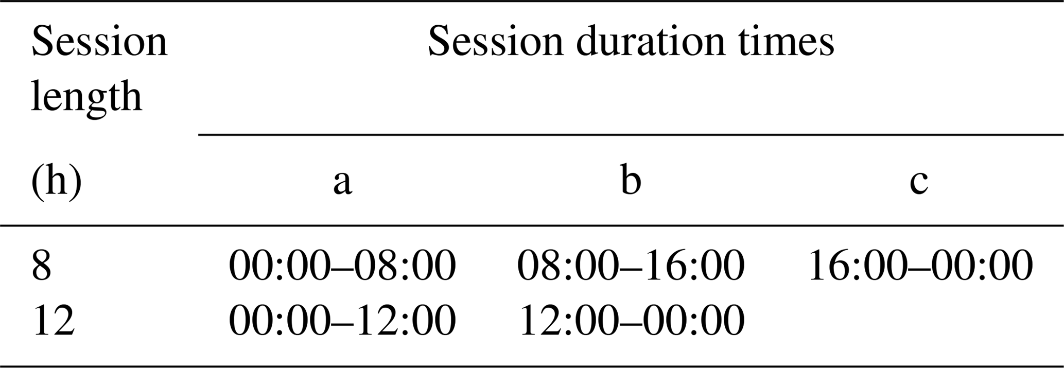
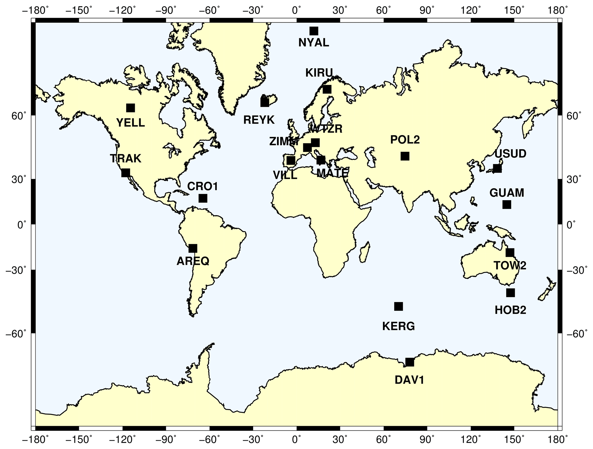
GPS data were downloaded in receiver-independent exchange (RINEX) format with 30 s intervals from the Scripps Orbit and Permanent Array Center (SOPAC), which is one of the data archives of the International GNSS Service (IGS) at http://sopac.ucsd.edu/ (last access: 15 October 2015). The IGS stations used in the study are demonstrated in Fig. 1. First of all, to determine the horizontal velocities for each of the stations we selected 3 successive days in October of each year for the years 2000 to 2015. Akarsu et al. (2015) did the similar sampling using only 1 day in a year. This is the procedure followed by many of the GPS experiments using repeated surveys (Aktuğ et al., 2009, 2013; Dogan et al., 2014; Koulali et al., 2015; McClusky et al., 2000; Ozener et al., 2010; Tatar et al., 2012). By using 3 consecutive days here, we believe we increased the reliability of the solutions. A treatment in regard to the solar activity, which was missing in Akarsu et al. (2015), was also taken into consideration (i.e. days with kappa index ≤4) here. In addition, 3 successive days in every month were included for the processing of the vertical component. In order to model the significant annual signal on GPS heights, here we did the sampling monthly. The GPS data were segmented into sub-sessions as listed in Table 1 in order to generate the repeated GPS measurements.

Table 1Segmented sub-sessions.

Download Print Version | Download XLSX

https://www.nat-hazards-earth-syst-sci.net/19/571/2019/nhess-19-571-2019-f01

Figure 1IGS continuous GPS sites used in the study.

Download

2.1.1 GAMIT/GLOBK processing

The GPS data were processed with GAMIT/GLOBK v10.6 software for relative point positioning (Herring et al., 2006 a, b) and with GIPSY-OASIS II v6.3 for PPP (Zumberge et al., 1997). The elevation cut-off angle was set to 7^∘ for both software packages.

The processing of the GPS data using GAMIT/GLOBK was conducted in three steps (Feigl et al., 1993; McClusky et al., 2000; Reilinger et al., 2006; Tatar et al., 2012; Dong et al., 1998; Cetin et al., 2018). We selected 18 globally scattered IGS stations. At first, the loosely constrained station coordinates, atmospheric zenith delays of each points, and Earth orientation parameters (EOPs) were estimated using doubly differenced GPS phase measurements and IGS final products. Global Pressure and Temperature 2 (GPT2) mapping function developed by Lagler et al. (2013) was used to model the delay in the atmosphere. The ocean tide loading correction was applied using the FES2004 model of Lyard et al. (2006). Ambiguities were on average resolved with 90 % success for the wide lane and 80 % success for the narrow lane (Fig. 2).

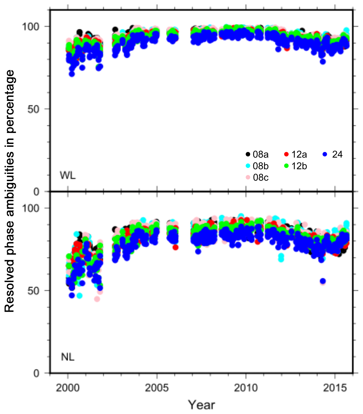
https://www.nat-hazards-earth-syst-sci.net/19/571/2019/nhess-19-571-2019-f02

Figure 2Daily fixed phase ambiguity resolution in percentage. WL is wide-lane ambiguity resolution and NL is narrow-lane ambiguity resolution.

Download

Secondly, GLOBK was used to estimate the point coordinates and velocities from a combined solution comprising the daily loosely constrained estimates, EOP values, orbit data, and their covariance through Kalman filtering. We used the IERS (International Earth Rotation and Reference Systems Service) Bulletin B values for Earth rotation parameters. Since our study was initially designed to be a global experiment, in this step we did not enlarge our network further with more globally scattered and loosely constrained IGS stations.

In the last step, the reference frame was realised on each day through generalised constraints. Iterations were applied to the initially chosen 18 IGS stations and about five bad sites were eliminated after four iterations. The reference frame was realised on each day, employing a reliable set of round 13 IGS stations in the ITRF2008 no-net-rotation (NNR) frame (Altamimi et al., 2012). The reliability of the IGS stations was characterised by GPS days which do not contain the effects of bad ionospheric conditions, with kappa index values smaller than 4, have at least 95 % data coverage, are available on the common days, and repeat on 3 consecutive days with overlapping sessions.

The processing strategies described above were applied to each subset of sessions listed in Table 1. The coordinate values for all sub-sessions were transformed to the topocentric system consisting of east, north, and up. The time series of the site ZIMM from relative positioning and PPP solutions for all sub-sessions were illustrated in Fig. 3.

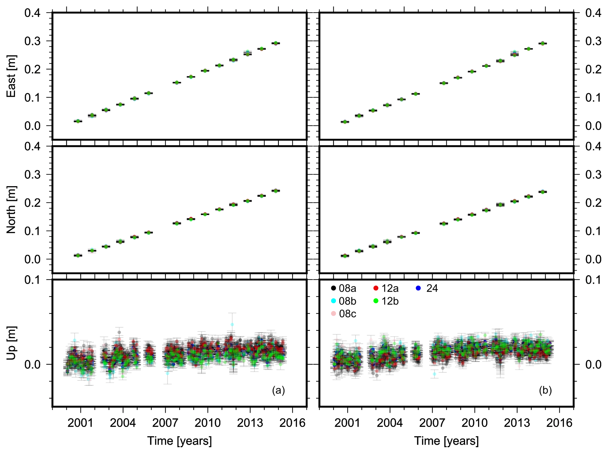
https://www.nat-hazards-earth-syst-sci.net/19/571/2019/nhess-19-571-2019-f03

Figure 3Time series of all sub-sessions for the site ZIMM from (a) relative positioning and (b) PPP solutions.

Download

2.1.2 GIPSY-OASIS II processing

We used JPL final precise (flinnR) orbits and clocks in the analysis. The (precise point positioning) PPP module of GIPSY-OASIS II v6.3 was developed by Zumberge et al. (1997). In GIPSY analysis, final orbits and clocks are determined from a global network solution. The results were represented using the International Earth Rotation Service's reference system ITRS (Petit and Luzum, 2010), as realised through the reference frame ITRF2008 (Altamimi et al., 2012). Tropospheric zenith wet delay was modelled as a random-walk parameter with a variance rate of 5 mm² h⁻¹ and wet delay gradient with a variance rate of 0.5 mm² h⁻¹. The dry troposphere was modelled using a priori zenith conditions of a GPT2 mapping function (Lagler et al., 2013). Pseudo-range and carrier phase observations were employed to eliminate the ionospheric delay using an L1 and L2 data combination. The Kedar et al. (2003) model was used to eliminate the effect of a second-order ionosphere. Satellite and receiver antenna phase centre variation (APV) maps were automatically applied following the IGS standards (Haines et al., 2010). The Desai (2002) model was used to eliminate the effect of ocean tide loading.

2.2 Velocity estimation and statistical tests

In this section, with the motivation from Akarsu et al. (2015), the estimation of an IGS site velocity and the related statistical tests will be explained. In Fig. 3, the comparison of all sub-session coordinate time series for all three GPS baseline components from both software results have been shown. Once the time series were looked at, all sub-sessions were in agreement. For the horizontal components that are east and north, the variations are almost perfectly linear, and this shows us the tectonic motion clearly. To estimate the linear variation (i.e. the velocity) the model of

\begin{matrix} (1) & x_{i} = a \cdot t_{i} + b + o_{i} \cdot x_{off} + v_{i} \end{matrix}

was used. There, x_i represents any coordinate value, a is site velocity, t_i is the time, b is the intercept, and v_i is the residuals. In a GPS solution time series there are additional terms such as to clarify the sudden displacements due to earthquakes. Then, Eq. (1) is expanded to include an offset value x_off and the corresponding coefficient o_i (Montillet et al., 2015). For instance in our analysis, the stations AREQ and USUD include offset values in their time series due to earthquakes. For all stations, the velocity estimations were calculated using Eq. (1) by means of the least-squares estimation.

The vertical component additionally includes significant seasonal variation. The coordinate time series for vertical components contain repeating annual cycles stemming from hydrological and atmospheric loading (Blewitt and Lavallée, 2002). Santamaría-Gómez et al. (2011) noticed seasonal motions in smaller periods like 3 and 4 months and diminishing amplitudes in GPS time series from continuously operating stations. Given these circumstances, it is not sufficient to determine vertical velocities with a linear model. The seasonal model we use here takes into account the annual and semi-annual periodicities:

\begin{array}{l} x_{i} & = a \cdot t_{i} + b + o_{i} \cdot x_{off} \\ (2) & + \sum_{n = 1}^{q} [c_{n} \cdot \cos \frac{2 π \cdot t_{i}}{T_{n}} + d_{n} \cdot \sin \frac{2 π \cdot t_{i}}{T_{n}}] + v_{i}, \end{array}

where q=2, T₁=1 year and T₂=0.5 year. The use of the offset parameter is the same as in the horizontal assessment. Furthermore, R², known as the coefficient of determination, was computed in a regression analysis as a statistical tool, which shows how well the data fit the estimated model. For any coordinate component from a regression analysis, the computation of R² is given with

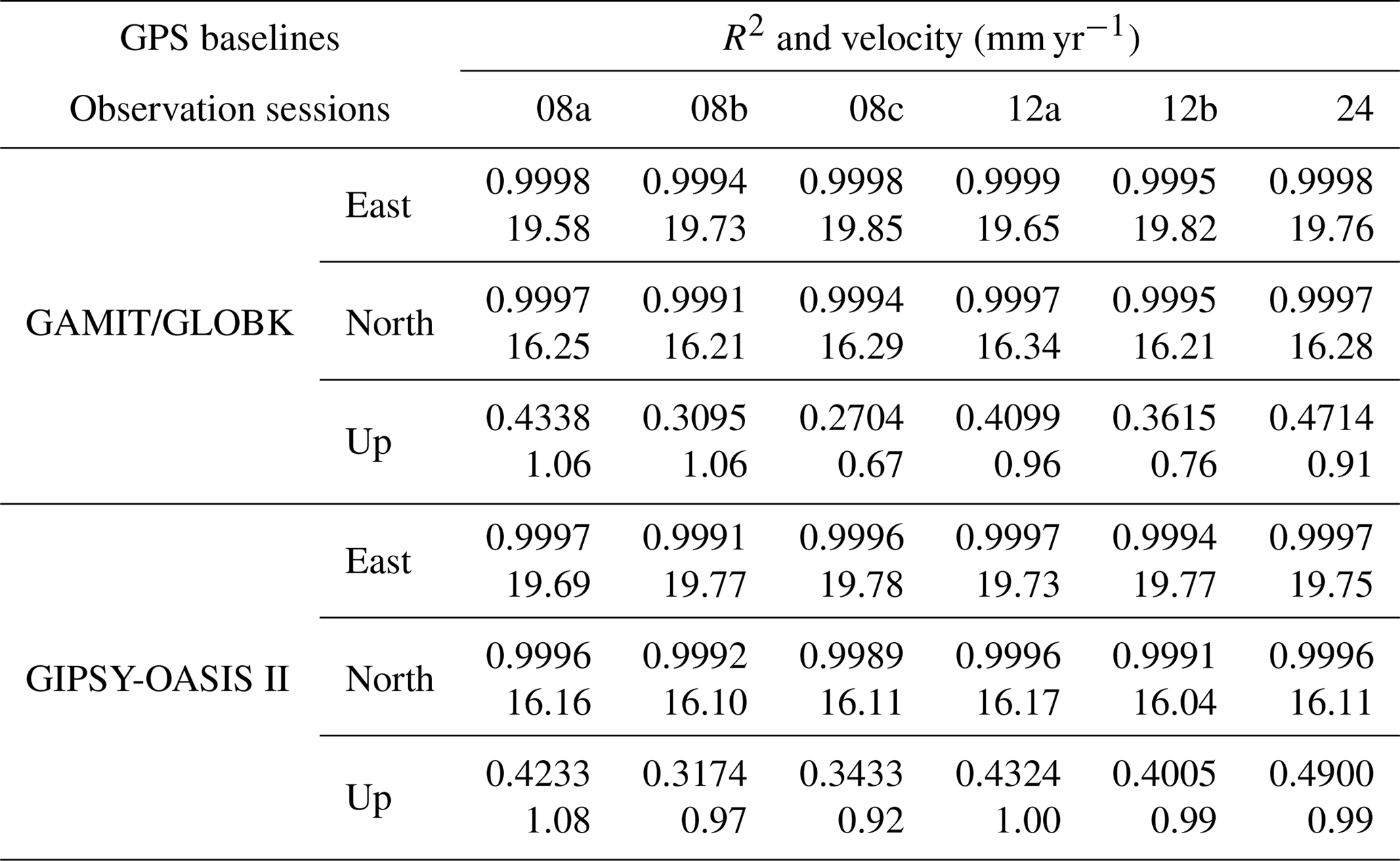
\begin{matrix} (3) & R^{2} = 1 - \frac{\sum_{i = 1}^{n} {\hat{v}}_{i}^{2}}{\sum_{i = 1}^{n} (x_{i} - \overline{x})^{2}} = 1 - \frac{\sum_{i = 1}^{n} (x_{i} - {\hat{x}}_{i})^{2}}{\sum_{i = 1}^{n} (x_{i} - \overline{x})^{2}}, \end{matrix}

where ${\hat{v}}_{i} = x_{i} - {\hat{x}}_{i}$ refers to the regression values ${\hat{x}}_{i} = \hat{a} t_{i} + \hat{b}$ based on the least-squares estimation ( $\sum_{i = 1}^{n} v_{i}^{2} = \min$ ), and $\overline{x}$ is the arithmetic average of n number of measurements used in the estimation. The velocity estimation results and R² values from both processing strategies for the station of ZIMM have been listed in Table 2. Almost all R² values of the horizontal components in Table 2 for both software are at the level of 0.99, whereas those of the vertical ones range from 0.27 to 0.49. It is because the up component is not as linear as the horizontal components. Furthermore, it is noisier due to the seasonal motion. Parallel to the low R² values, the estimated velocities also have a larger fluctuation for the vertical component.

Table 2Site velocities and R² values from both solutions for the site ZIMM.

Download Print Version | Download XLSX

For all the stations in the IGS network, the solutions from sub-sessions were compared with the solutions (i.e. velocities) of 24 h accepted as the truth. The statistical assessments of hypotheses were carried out in three steps. Then, the equivalency between the unit variance derived from LSE of the sub-session given in Table 1 and that of the 24 h session was tested. The relevant hypothesis testing was set to be $H_{0} : σ_{24}^{2} = σ_{s}^{2}$ and $H_{A} : σ_{24}^{2} \neq σ_{s}^{2}$ , where σ² represents the unit variance and subscripts represent the observation session. A hypothesis testing based on an F distribution was applied to check the equivalency of the variances. In the case that unit variances were found to be equivalent, Student's t test was applied whether or not the velocity estimated from the campaign GPS significantly differs from the velocity derived from continuous GPS. The null hypothesis was set to be ( $H_{0} : a_{24} = a_{s}$ ) against the alternative hypothesis ( $H_{0} : a_{24} \neq a_{s}$ ), where a_i denotes the velocity values in Eqs. (1) and (2). Briefly, it was tested whether or not there is a significant difference between the results of 24 h solutions and those of the sub-sessions. In these statistical tests, the degree of freedom values for the horizontal components were approximately 42, whereas the degree of freedom for the vertical component was about 345. The degree of freedom varied with respect to the number of insignificant parameters from the LSE.

3 Results and discussion

As described in the previous section, the time series generated from all sessions of each continuous GPS site were analysed. The coefficient of determination (i.e. R²), which shows how well the data fit the model, is computed according to Eq. (3). Tables 3, 4, and 5 compare the results of sub-sessions with those of the 24 h statistically. Tables generally consist of two columns, which includes the relative evaluation results from GAMIT/GLOBK v10.60 and the PPP results from GIPSY-OASIS II v6.3 software. In each column, R² values and hypothesis test results are given.

Table 3For the north component, R² values and hypothesis test results for relative positioning and PPP.

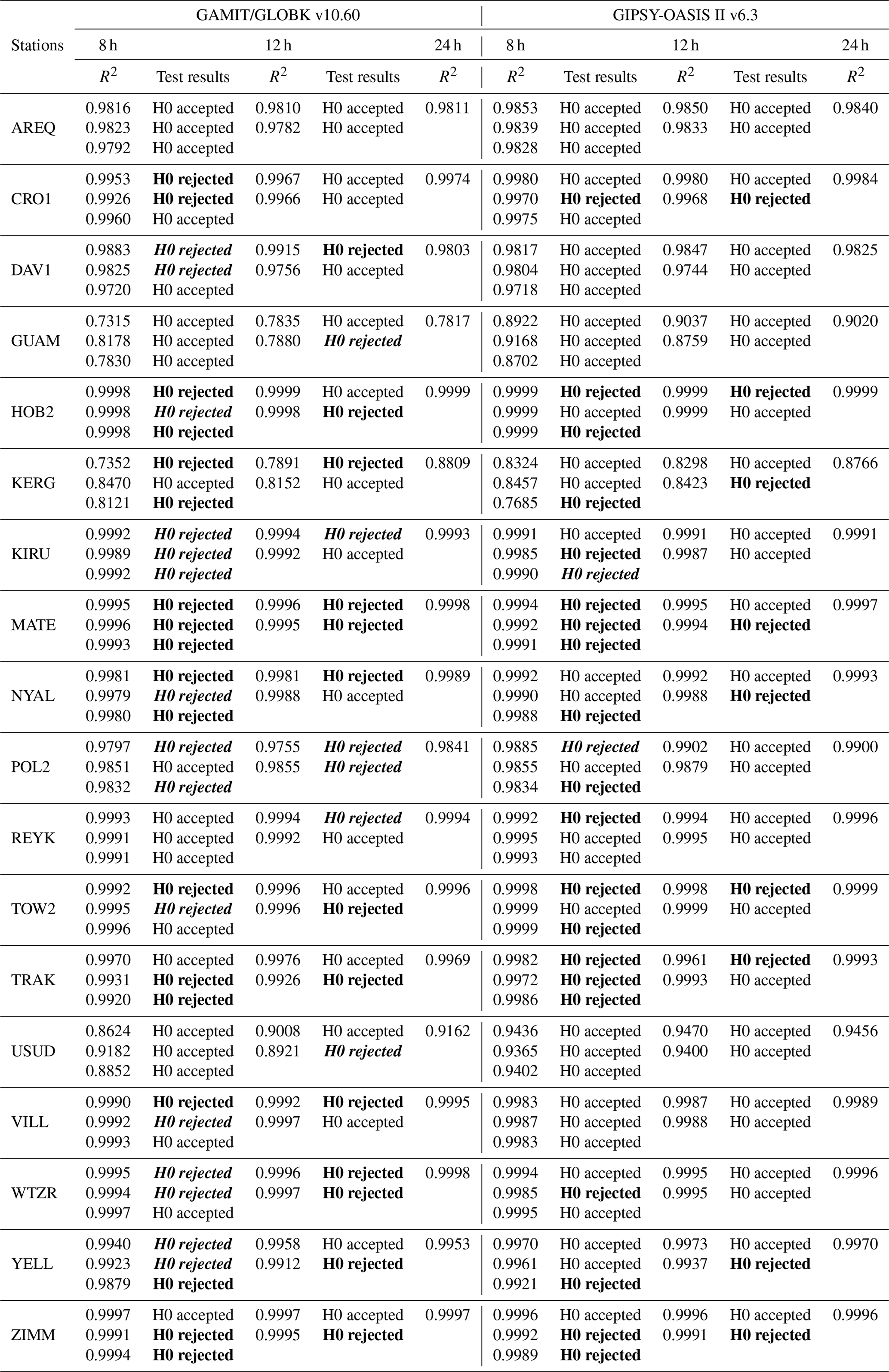
Download Print Version | Download XLSX

Table 4For the east component, R² values and hypothesis test results for relative positioning and PPP.

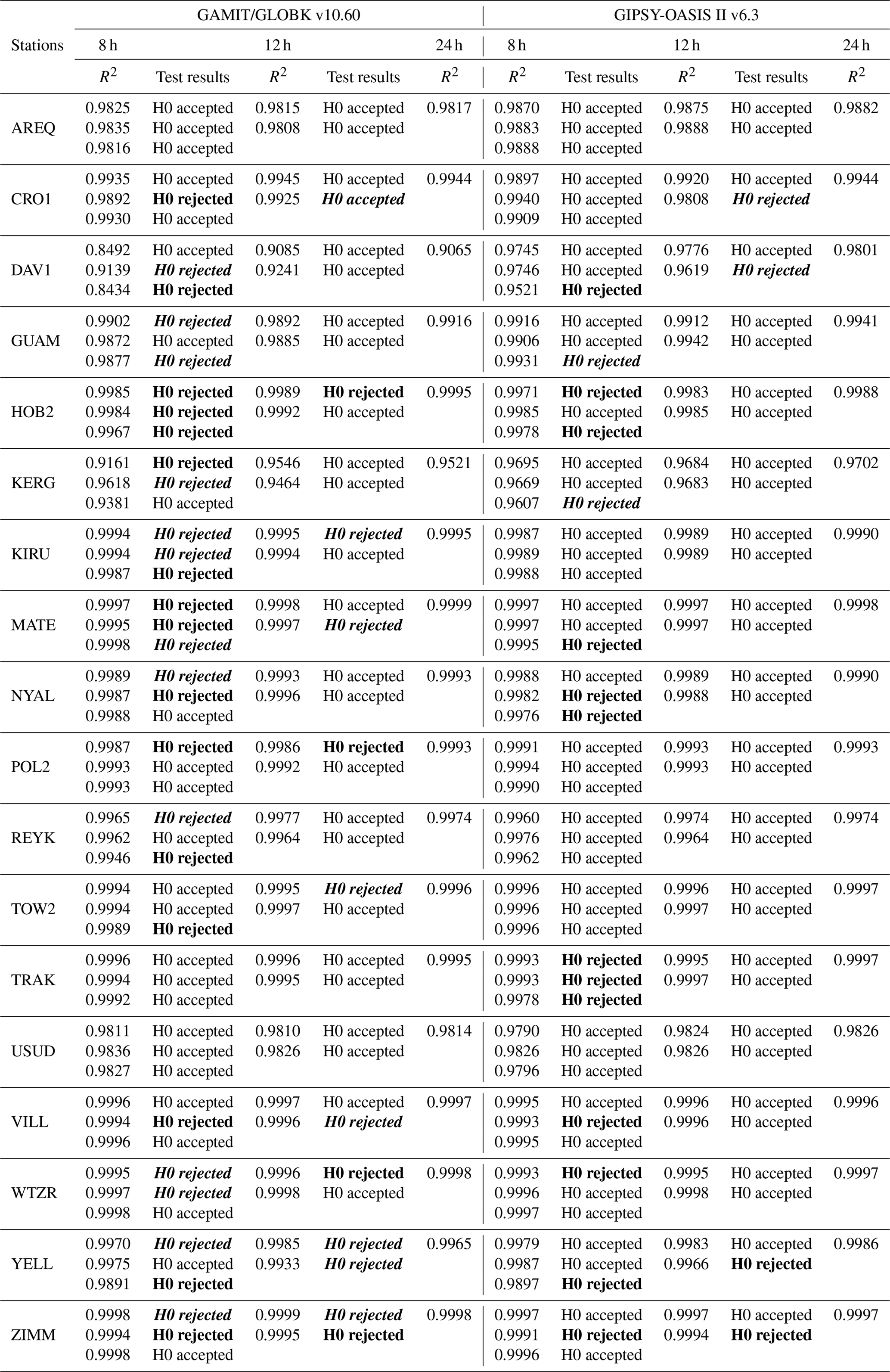
Download Print Version | Download XLSX

Table 5For the up component, R² values and hypothesis test results for relative positioning and PPP.

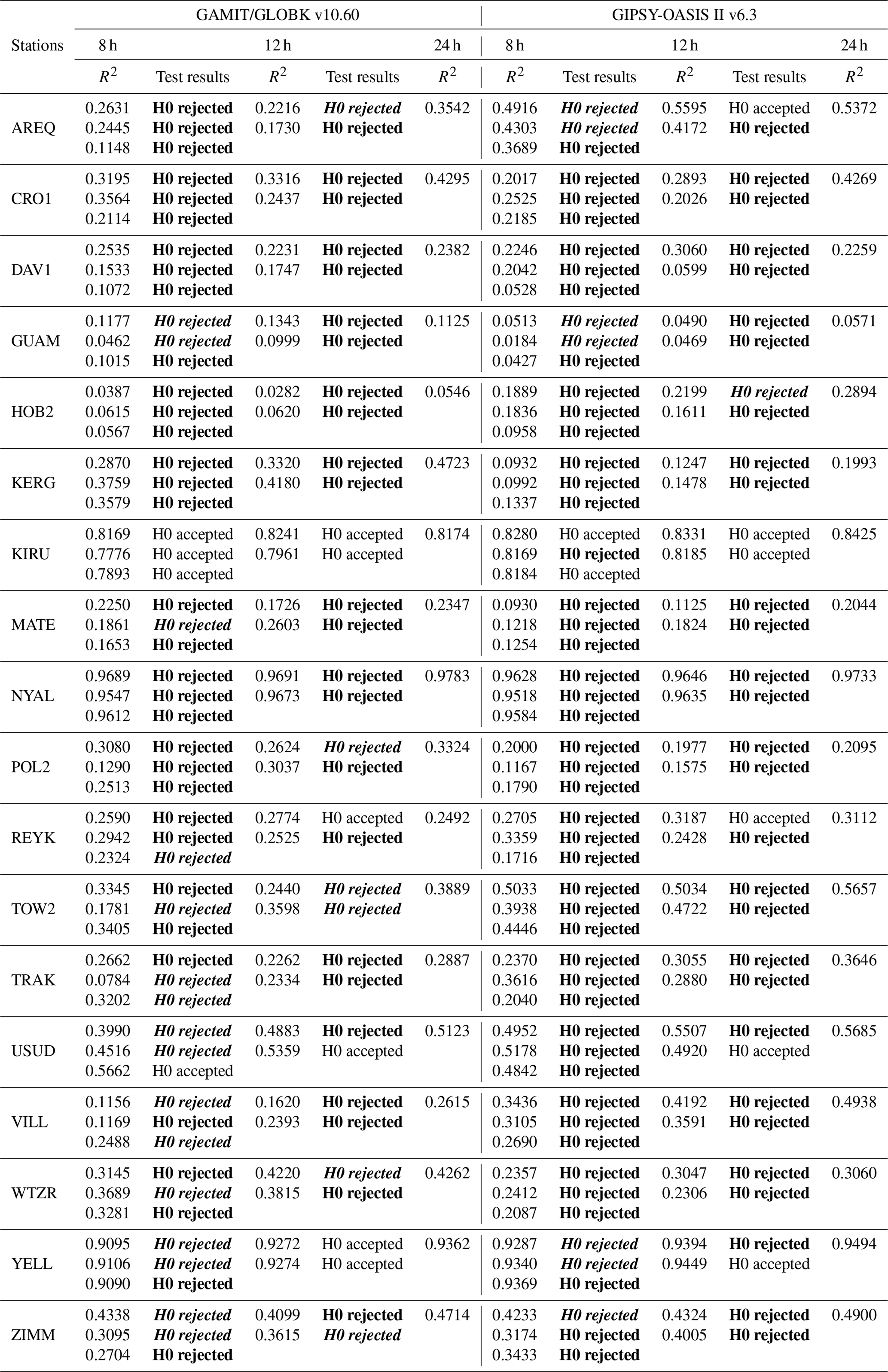
Download Print Version | Download XLSX

Hypothesis test results are based on a 95 % confidence level. If the hypothesis H₀ is accepted, it is shown that there is no statistically significant difference from the geodetic site velocities from sub-sessions to those from 24 h session results. If the hypothesis H₀ is rejected (only expressed in bold), a posteriori unit variance obtained from the least-squares estimation is statistically different from the 24 h one based on the F test; that is, the models used for the geodetic velocity estimation are not equivalent. Furthermore, both the results expressed in bold and italic indicate that the model is equivalent, but the deformation rate from the 24 h session is statistically different from the velocities from the sub-sessions based on Student's t test.

In Fig. 3, the subplots of the horizontal component clearly show the character of the tectonic motion linearly. In this context, once Tables 4 and 5 are examined, it is obviously seen that R² values estimated from all sessions are close to 1, except for GUAM, KERG, USUD (in Table 4), and DAV1 (in Table 5). For instance, the motion in USUD is thought to be due to the post-seismic relaxation.

Success rates of velocity estimation from PPP and relative positioning are illustrated in Fig. 4. There, blue bars are for 8 h and orange bars are for 12 h sessions. With the success rate here, we mean the success of velocity estimation from short sessions when the velocity estimation from 24 h is taken as the truth. The dashed pattern shows PPP results, whereas no pattern is for relative positioning. First of all, success rates for the horizontal components vary from 40 % to 90 %. Furthermore, the rates from 12 h sessions are higher than those of the 8 h sessions as expected. Note that the horizontal success rates from PPP are higher than those of the relative positioning, formed over long baselines to use in tectonic studies.

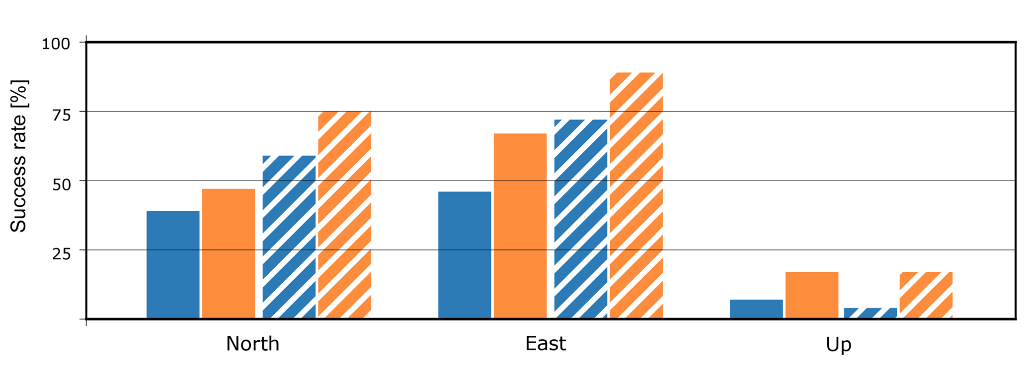
https://www.nat-hazards-earth-syst-sci.net/19/571/2019/nhess-19-571-2019-f04

Figure 4Success rates of 8 h and 12 h sessions. The velocity estimation from short sessions is compared with 24 h results for each GPS component. Blue bars are for the 8 h and orange bars are for the 12 h sessions. Dashed patterns illustrate PPP estimates, whereas no patterns are for the relative positioning.

Download

The fact that the accuracy of the vertical component is worse than that of the horizontal component is often expressed in the literature and in practice by many researchers. Therefore, the repeatabilities for this component are larger, and the seasonal effects are much more apparent than the horizontal ones. For this reason, the values of R² in Table 5 are much lower than those calculated from the horizontal component (around 0.40). Likewise, the results of the hypothesis test were rejected at a higher rate. Both for PPP and relative positioning, success rates for the vertical component are low, varying from about 5 % to 15 %. These rates are almost the same for both methods.

Overall, the success rates of 12 h solutions are higher than those of the 8 h solutions, and the systematic effect acting on shorter sessions is varied and greater. For both positioning methods, the east component has greater success than the north one with regard to the truth. The success rates in Fig. 4 are higher for PPP than relative positioning because in the GAMIT/GLOBK processing long baseline lengths are formed. Over long baseline lengths, troposphere and ionosphere modelling become difficult, orbit errors accumulate, and hence ambiguity resolution becomes worse.

The reliability of velocity estimation from short GPS campaigns using PPP has been improved here when comparing results with those of Akarsu et al. (2015). By the improvement we mean that the statistical agreement between the velocity estimated from short GPS observations and those of 24 h sessions is higher here. The improvement in the horizontal component is 35 % and 40 % for 8 and 12 h respectively. The vertical component was improved by 4 % and 17 % for 8 and 12 h. This improvement might be ascribed to a few developments in the analysis procedures. First of all, here we used GPS time series from 2000. In other words, the noisier part, 1990–2000, is eliminated, which might have affected the quality of estimated velocities in Akarsu et al. (2015). Second, the analysis was performed with reprocessed orbits and clocks. JPL changed its orbit and clock estimation strategy as of the year 2007 (Hayal and Sanli, 2016). Third, GIPSY single-receiver ambiguity resolution further improved the accuracy of PPP (Bertiger et al., 2010). Bertiger et al. (2010) and Hayal and Sanli (2016) showed how positioning accuracy was improved with reprocessed JPL products and single-receiver ambiguity resolution. Reprocessing especially improved the east component and this is correlated with the findings in this paper. Fourth, campaign measurements were performed over 3 consecutive days (i.e. the sampling was made such that IGS data were processed selecting 3 consecutive days from the archive). Therefore, it was possible to eliminate the outlier solution from the processing. Finally, GPS campaigns were selected from the days on which the effect of geomagnetic storms is eliminated.

Eckl et al. (2001) showed that using proper ambiguity resolution, troposphere modelling, and IGS precise orbits relative positioning performs uniformly; i.e. it is not dependent on baseline length for baseline lengths shorter than 300 km. In this experiment, GAMIT/GLOBK relative positioning used baseline lengths longer than 300 km. This degraded the accuracy of positioning and hence the velocity estimation of relative positioning. This was even achieved with slightly coarser accuracy than the PPP positioning. Based on relative positioning, BERNESE processing also gave similar results in Duman and Sanli (2016). Many studies in the literature monitoring tectonics with long baselines to stable plates need to take this into account (Ayhan et al., 2002; Aktuğ et al., 2015; Reilinger et al., 2006; Ozener et al., 2010).

4 Conclusions

We incorporated relative positioning in the determination of the accuracy of GPS site velocities from GPS campaigns (i.e. observation sessions shorter than 24 h). Relative positioning results were produced from GAMIT/GLOBK. The results were also compared with PPP solutions derived from GIPSY-OASIS II. A global experiment for proper sampling was adopted using the IGS network.

The results indicate that relative positioning using long baseline lengths and short observation sessions produces similar results to PPP. The accuracy is slightly coarser for horizontal positioning and slightly better for vertical positioning. Previously it has been noted that the accuracy of relative positioning does not depend on baseline length if baselines are shorter than 300 km. In the GAMIT/GLOBK processing here, reference points were chosen that were longer than 300 km.

It has also been noted that the accuracy of GPS site velocities derived from short observation sessions using PPP was improved here compared to previous studies. This is ascribed to the fact that the new GIPSY PPP runs with a new ambiguity resolution algorithm called single-receiver ambiguity resolution. This especially improved the east component and the east results in this study show better accuracy. Furthermore, the analysis was performed using reprocessed JPL orbits and clocks. The contribution of reprocessed JPL products to positioning was previously discussed among researchers. Differing from the previous studies, our sampling here also comprises GPS days freed from the effect of geomagnetic storms. In addition, repeating campaign GPS measurements over 3 consecutive days helps us to remove a bad solution from the analysis. The noisier IGS time series between 1990 and 2000 was not used. If the user takes into account the above-listed factors in the planning of their fieldwork they should expect similar types of accuracy levels.

In this study, the horizontal velocity accuracy of GPS campaigns with 12 h observation sessions from PPP seems to reach a confidence level of about 85 %. However, the reliability of vertical velocities is very poor and at about 20 %. This means that tectonic studies trying to use the daylight as the observation duration would still produce poorer accuracy than the expected 95 %. Of course, as this result is based on GPS solutions only, one should expect levels of 95 % once solutions are compiled from multi-GNSS experiments. Although the accuracy of velocity estimation was improved about 40 % for horizontal positioning and 20 % for vertical positioning, it is still not at the desired confidence level.

Data availability

The data used in this paper are accessible at http://sopac.ucsd.edu/ (last access: 15 October 2015).

Author contributions

HD did the analysis, prepared all tables and figures as well as writing the original manuscript. DUS set the hypothesis, supervised the study and recompiled the original manuscript.

Competing interests

The authors declare that they have no conflict of interest.

Acknowledgements

The authors are grateful to the IGS for the distribution of GNSS data and to SOPAC for a perfect data archiving service. The figures were plotted using the Generic Mapping Tools and we express our gratitude to the open-source software designers. We extend our gratitude to Fatih Poyraz for the valued discussions on GAMIT/GLOBK processing. We also would like to thank the two anonymous reviewers for their constructive comments.

Review statement

This paper was edited by Filippos Vallianatos and reviewed by two anonymous referees.

References

Akarsu, V., Sanli, D. U., and Arslan, E.: Accuracy of velocities from repeated GPS measurements, Nat. Hazards Earth Syst. Sci., 15, 875–884, https://doi.org/10.5194/nhess-15-875-2015, 2015. a, b, c, d, e, f, g, h

Aktuğ, B., Kiliçoğlu, A., Lenk, O., and Gürdal, M. A.: Establishment of regional reference frames for quantifying active deformation areas in Anatolia, Stud. Geophys. Geod., 53, 169–183, https://doi.org/10.1007/s11200-009-0011-0, 2009. a

Aktuğ, B., Meherremov, E., Kurt, M., Özdemir, S., Esedov, N., and Lenk, O.: GPS constraints on the deformation of Azerbaijan and surrounding regions, J. Geodyn., 67, 40–45, https://doi.org/10.1016/j.jog.2012.05.007, 2013. a

Aktuğ, B., Doğru, A., Özener, H., and Peyret, M.: Slip rates and locking depth variation along central and easternmost segments of North Anatolian Fault, Geophys. J. Int., 202, 2133–2149, https://doi.org/10.1093/gji/ggv274, 2015. a

Altamimi, Z., Métivier, L., and Collilieux, X.: ITRF2008 plate motion model, J. Geophys. Res.-Sol. Ea., 117, B07402, https://doi.org/10.1029/2011JB008930, 2012. a, b

Ashurkov, S. V., San'kov, V. A., Miroshnichenko, A. I., Lukhnev, A. V., Sorokin, A. P., Serov, M. A., and Byzov, L. M.: GPS geodetic constraints on the kinematics of the Amurian Plate, Russ. Geol. Geophys., 52, 239–249, 2011. a

Ayhan, M. E., Demir, C., Lenk, O., Kilicoglu, A., Altiner, Y., Barka, A. A., and Ozener, H.: Interseismic strain accumulation in the Marmara Sea region. B. Seismol. Soc. Am., 92, 216–229, 2002. a

Bertiger, W., Desai, S. D., Haines, B., Harvey, N., Moore, A. W., Owen, S., and Weiss, J. P.: Single receiver phase ambiguity resolution with GPS data, J. Geodesy., 84, 327–337, 2010. a, b

Bingley, R., Dodson, A., Penna, N., Teferle, N., and Baker, T.: Monitoring the vertical land movement component of changes in mean sea level using GPS: results from tide gauges in the UK, Journal of Geospatial Engineering, 3, 9–20, 2001. a, b

Bitharis, S., Fotiou, A., Pikridas, C., and Rossikopoulos, D.: A New Velocity Field of Greece Based on Seven Years (2008–2014) Continuously Operating GPS Station Data, in: International Symposium on Earth and Environmental Sciences for Future Generations, Springer, Cham, 321–329, 2016. a

Blewitt, G. and Lavallée, D.: Effect of annual signals on geodetic velocity, J. Geophys. Res.-Sol. Ea., 107, 9-1–9-11, 2002. a

Catalão, J., Nico, G., Hanssen, R., and Catita, C.: Merging GPS and atmospherically corrected InSAR data to map 3-D terrain displacement velocity, IEEE T. Geosci. Remote, 49, 2354–2360, 2011. a

Cetin, S., Aydin, C., and Dogan, U.: Comparing GPS positioning errors derived from GAMIT/GLOBK and Bernese GNSS software packages: A case study in CORS-TR in Turkey, Survey Review, Online Published, doi:10.1080/00396265.2018.1505349, 2018. a

Chousianitis, K., Ganas, A., and Evangelidis, C. P.: Strain and rate patterns of mainland Greece from continuous GPS data and comparison between seismic and geodetic moment release, J. Geophys. Res.-Sol. Ea., 120, 3909–3931, 2015. a

Desai, S. D.: Observing the pole tide with satellite altimetry, J. Geophys. Res.-Oceans, 107, 7–1, 2002. a

Dixon, T. H., Miller, M., Farina, F., Wang, H., and Johnson, D.: Present-day motion of the Sierra Nevada block and some tectonic implications for the Basin and Range province, North American Cordillera, Tectonics, 19, 1–24, 2000. a, b, c, d

Dogan, U., Demir, D. Ö., Çakir, Z., Ergintav, S., Ozener, H., Akoğlu, A. M., Nalbant, S. S., and Reilinger, R.: Postseismic deformation following the M_w 7.2, 23 October 2011 Van earthquake (Turkey): Evidence for aseismic fault reactivation, Geophys. Res. Lett., 41, 2334–2341, 2014. a

Dong, D., Herring, T., and King, R.: Estimating regional deformation from a combination of space and terrestrial geodetic data, J. Geodesy., 72, 200–214, 1998. a

Duman, H. and Sanli, D. U.: Accuracy of velocities from repeated GPS surveys: relative positioning is concerned, EGU General Assembly Conference Abstracts, Vol. 18, 23–28 April 2016, Vienna, Austria, 2016. a

Eckl, M., Snay, R., Soler, T., Cline, M., and Mader, G.: Accuracy of GPS-derived relative positions as a function of interstation distance and observing-session duration, J. Geodesy., 75, 633–640, 2001. a

Elliott, J. L., Larsen, C. F., Freymueller, J. T., and Motyka, R. J.: Tectonic block motion and glacial isostatic adjustment in southeast Alaska and adjacent Canada constrained by GPS measurements, J. Geophys. Res.-Sol. Ea., 115, B09407, https://doi.org/10.1029/2009JB007139, 2010. a

Feigl, K. L., Agnew, D. C., Bock, Y., Dong, D., Donnellan, A., Hager, B. H., Herring, T. A., Jackson, D. D., Jordan, T. H., and King, R. W.: Space geodetic measurement of crustal deformation in central and southern California, 1984–1992, J. Geophys. Res.-Sol. Ea., 98, 21677–21712, 1993. a

Haines, B., Bar-Sever, Y., Bertiger, W., Desai, S., Harvey, N., and Weiss, J.: Improved models of the GPS satellite antenna phase and group-delay variations using data from low-earth orbiters, AGU fall meeting, 13–17 December 2010, San Francisco, California, USA, 2010. a

Hayal, A. G. and Sanli, D. U.: Revisiting the role of observation session duration on precise point positioning accuracy using GIPSY/OASIS II Software, B. Cienc. Geod., 22, 405–419, 2016. a, b

Herring, T. A., King, R. W., and McClusky, S.: Documentation For The GAMIT GPS Analysis Software, Massachusetts Institute of Technology, ABD, Massachusetts, 2006a. a

Herring, T. A., King, R. W., and McClusky, S.: Documentation For The GLOBK GPS Analysis Software, Massachusetts Institute of Technology, ABD, Massachusetts, 2006b. a

Hollenstein, C., Müller, M. D., Geiger, A., and Kahle, H. G.: Crustal motion and deformation in Greece from a decade of GPS measurements, 1993–2003, Tectonophysics, 449, 17–40, 2008. a

Kedar, S., Hajj, G. A., Wilson, B. D., and Heflin, M. B.: The effect of the second order GPS ionospheric correction on receiver positions, Geophys. Res. Lett., 30, B07402, https://doi.org/10.1029/2003GL017639, 2003. a

Koulali, A., Tregoning, P., McClusky, S., Stanaway, R., Wallace, L., and Lister, G.: New Insights into the present-day kinematics of the central and western Papua New Guinea from GPS, Geophys. J. Int., 202, 993–1004, 2015. a

Lagler, K., Schindelegger, M., Böhm, J., Krásná, H., and Nilsson, T.: GPT2: Empirical slant delay model for radio space geodetic techniques, Geophys. Res. Lett., 40, 1069–1073, 2013. a, b

Lyard, F., Lefevre, F., Letellier, T., and Francis, O.: Modelling the global ocean tides: modern insights from FES2004, Ocean Dynam., 56, 394–415, 2006. a

Mao, A., Harrison, C. G., and Dixon, T. H.: Noise in GPS coordinate time series. J. Geophys. Res.-Sol. Ea., 104, 2797–2816, 1999. a, b, c

McClusky, S., Balassanian, S., Barka, A., Demir, C., Ergintav, S., Georgiev, I., Gurkan, O., Hamburger, M., Hurst, K., and Kahle, H.: Global Positioning System constraints on plate kinematics and dynamics in the eastern Mediterranean and Caucasus, J. Geophys. Res.-Sol. Ea., 105, 5695–5719, 2000. a, b

Miranda, J. M., Navarro, A., Catalão, J., and Fernandes, R. M. S.: Surface displacement field at Terceira Island deduced from repeated GPS measurements. J. Volcanol. Geoth. Res., 217, 1–7, 2012. a

Montillet, J.-P., Williams, S., Koulali, A., and McClusky, S.: Estimation of offsets in GPS time-series and application to the detection of earthquake deformation in the far-field, Geophys. J. Int., 200, 1207–1221, 2015. a

Ozener, H., Arpat, E., Ergintav, S., Dogru, A., Cakmak, R., Turgut, B., and Dogan, U.: Kinematics of the eastern part of the North Anatolian Fault Zone, J. Geodyn., 49, 141–150, 2010. a, b

Ozener, H., Dogru, A., and Acar, M.: Determination of the displacements along the Tuzla fault (Aegean region-Turkey): Preliminary results from GPS and precise leveling techniques, J. Geodyn., 67, 13–20, 2013. a

Petit, G. and Luzum, B.: IERS Conventions (2010), IERS Technical Note 36, Int. Earth Rotation Serv., Paris, 179 pp., 2010. a

Reilinger, R. E., McClusky, S. C., Oral, M. B., King, R. W., Toksoz, M. N., Barka, A. A., and Sanli, I.: Global Positioning System measurements of present-day crustal movements in the Arabica-Africa-Eurasia plate collision zone, J. Geophys. Res.-Sol. Ea., 102, 9983–9999, 1997. a

Reilinger, R., McClusky, S., Vernant, P., Lawrence, S., Ergintav, S., Cakmak, R., Ozener, H., Kadirov, F., Guliev, I., and Stepanyan, R.: GPS constraints on continental deformation in the Arabica-Africa-Eurasia continental collision zone and implications for the dynamics of plate interactions, J. Geophys. Res.-Sol. Ea., 111, B05411, https://doi.org/10.1029/2005JB004051, 2006. a, b

Rontogianni, S.: Comparison of geodetic and seismic strain rates in Greece by using a uniform processing approach to campaign GPS measurements over the interval 1994–2000, J. Geodyn., 50, 381–399, 2010. a

Santamaría-Gómez, A., Bouin, M. N., Collilieux, X., and Wöppelmann, G.: Correlated errors in GPS position time series: implications for velocity estimates, J. Geophys. Res.-Sol. Ea., 116, B01405, https://doi.org/10.1029/2010JB007701, 2011. a

Serpelloni, E., Vannucci, G., Pondrelli, S., Argnani, A., Casula, G., Anzidei, M., Baldi, P., and Gasperini, P.: Kinematics of the Western Africa-Eurasia plate boundary from focal mechanisms and GPS data, Geophys. J. Int., 169, 1180–1200, 2007. a

Tatar, O., Poyraz, F., Gürsoy, H., Cakir, Z., Ergintav, S., Akpınar, Z., Koçbulut, F., Sezen, F., Türk, T., and Hastaoğlu, K. Ö.: Crustal deformation and kinematics of the Eastern Part of the North Anatolian Fault Zone (Turkey) from GPS measurements, Tectonophysics, 518, 55–62, 2012. a, b

Tran, D. T., Nguyena, T. Y., Duongb, C. C., Vya, Q. H., Zuchiewiczc, W., Cuonga, N. Q., and Nghiac, N. V.: Recent crustal movements of northern Vietnam from GPS data. J. Geodyn., 69, 5–10, 2013. a

Vernant, P., Nilforoushan, F., Hatzfeld, D., Abbassi, M. R., Vigny, C., Masson, F., Nankali, H., Martinod, J., Ashtiani, A., Bayer, R., Tavakoli, F., Chéry, J.: Present-day crustal deformation and plate kinematics in the Middle East constrained by GPS measurements in Iran and northern Oman, Geophys. J. Int., 157, 381–398, 2004. a

Zhang, J., Bock, Y., Johnson, H., Fang, P., Williams, S., Genrich, J., and Behr, J.: Southern California Permanent GPS Geodetic Array: Error analysis of daily position estimates and site velocities, J. Geophys. Res.-Sol. Ea., 102, 18035–18055, 1997. a, b, c, d, e, f

Zumberge, J., Heflin, M., Jefferson, D., Watkins, M., and Webb, F. H.: Precise point positioning for the efficient and robust analysis of GPS data from large networks, J. Geophys. Res.-Sol. Ea., 102, 5005–5017, 1997. a, b

Articles

Short summary

Research has been done to assess the performance of relative positioning over long baseline lengths in determining the accuracy of site velocities from GPS campaign measurements. GPS campaign measurements were generated from the IGS data, and the results were compared with PPP-derived findings. A major outcome of this study is that relative positioning over long baseline lengths produces similar accuracies to PPP. A newly proposed refinement method also improves the available PPP accuracy.