2.1 The EURO-CORDEX ensemble

EURO-CORDEX at 0.11^∘ spatial resolution is the current state-of-the-art regional climate model ensemble over Europe. The ensemble is the result of the cooperation between many European institutions, and further ensemble members are still being added. Here, we are limited to a subset of the ensemble with members for which we have received precipitation data at a 1 h temporal resolution; see Table 1. This subset is not including the common reanalysis downscaling simulations, and the analysis is therefore of GCM–RCM combinations, which introduce some additional uncertainties (Déqué et al., 2012).

Table 1The RCM–GCM simulations with hourly precipitation output that are included in the analysis. The experiment code (“rip nomenclature”) from CMIP5 indicates the realization (r), the initialization (i), and the physics set-up (p) used. Here, the code is listed due to differences in the realizations of the EC-Earth model.

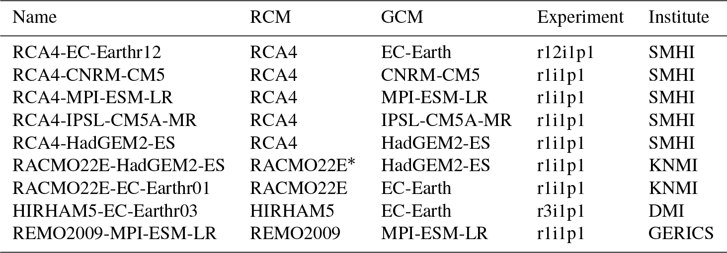
^* Version 2 (v2) of the simulation as submitted to the Earth System Grid Federation (ESGF).

Download Print Version | Download XLSX

Kotlarski et al. (2014) give an overview of the details of the models and applied parameterizations, such as the different convective parameterizations used by the models. In the paper, they also present the performance of the RCMs in reanalysis-driven simulations, mainly discussing average quantities of precipitation and temperature. Focusing on their results for the summer season, the RCMs in the sub-ensemble used here follow the general pattern of a warm summer bias in REMO2009 in continental Europe, whereas RACMO22E has a general cold bias, and RCA4 and HIRHAM5 are too warm in the south and too cold in the north. Bias in precipitation is more scattered but follows a similar structure as the temperature bias for each of the models, indicating a strong dependency of cold and wet conditions, as can be expected for mean quantities. Prein et al. (2016) show that model bias in the EURO-CORDEX 0.11^∘ simulations are reduced compared to the earlier 0.44^∘ simulations, for both mean and extreme daily and 3-hourly precipitation, especially in local areas. Rajczak and Schär (2017) analysed heavy and extreme daily precipitation intensity and found good performance in RCMs, mostly independent of the driving GCM.

Jacob et al. (2014) investigated end-of-century climate change for the EURO-CORDEX 0.11^∘ simulations, with significant changes in both mean precipitation and temperature across Europe for RCP4.5 and RCP8.5. Whereas mean precipitation generally increases in northern Europe and decreases in southern Europe, heavy precipitation shows robust changes across the ensemble, with significant increases in north-eastern Europe in summer, and pan-European increases in winter under RCP8.5. Kjellström et al. (2018) investigated climate change patterns as a function of global mean temperature increases of 1.5 and 2.0 ^∘C, with similar results for mean precipitation and temperature as in Jacob et al. (2014). Projected precipitation extremes were investigated by Dosio (2015) and showed general increases in the annual top daily extremes and in the 95th percentile of the precipitation distribution.

The presented analysis makes use of a historical period from 1971 to 2000, as well as future scenario periods 2011–2040, 2041–2070, and 2071–2100. The analysis is restricted to summer half-years (April–September), which constitutes the main convective seasons for large parts of Europe (Berg et al., 2009). Unfortunately, as pointed out in the review process of the current paper, this interferes with the main convective season during autumn in southern France (Berthou et al., 2018) and parts of the Mediterranean. The results for those regions must therefore be handled with caution, especially in a future climate where the seasonality might shift to even later in the year (Marelle et al., 2018). RCP4.5 and RCP8.5 are investigated for all models.

2.2 National DDF data

The model simulations are evaluated against gauge based DDF curves as obtained from countries across Europe, namely Austria, Germany, Sweden, the Netherlands, and France. Much of the information about how the DDFs were calculated is only available in local languages, and the exact procedures are sometimes not clearly or sufficiently explained. Below, we provide a brief introduction to each data set but refer to references for details.

3.1 Durations

The DDF statistics are derived in a conventional way by employing a running window with a given duration to arrive at the peak intensity over that window; a so-called “block rain”, which does not reflect the actual event durations. We are confined here to a base resolution of 1 h, which means that the 1-hourly duration is simply taking 1 h steps and that no running mean is possible. This gives an inherent underestimation of the true hourly DDF statistics. For durations above 1 h (2, 3, 6, and 12 h are studied), the running window progresses at 1 h steps, giving a steadily more accurate estimate of the peak intensity.

3.2 Extreme value theory approach

Extreme value theory is applied to study precipitation extremes at various durations. Within extreme value theory, there are two main paths normally taken when it comes to precipitation analyses: annual maxima (AM) or POT (also called partial duration series, PDS) (Coles et al., 2001). With the AM approach (often called block maxima) a single event is selected within a block of data, typically within 1 year for geophysical time series, and with the POT approach a number of events with values greater than a given threshold are selected. The latter allows multiple events in a given year to be selected, and additional choices must be made to assure that the samples are independent and identically distributed (iid). To achieve iid samples, a minimum time separation, t_s, is prescribed such that two events cannot occur too close in time. The time separation varies with the duration, d, in hours, such that

A total time range of (d+2t_s(d)) h is thereby excluded from further analysis. The selected separation time is set higher than in many studies based on higher temporal resolution data (e.g. Dunkerley, 2008). Further, it is also set conservatively compared to studies based on actual event durations, i.e. defined as periods of hours from increase above a set threshold until below that threshold (Medina-Cobo et al., 2016), in contrast with the block rain approach used here. Other studies using climate model data have used even more conservative de-clustering times of 1 or 2 d (Ban et al., 2018; Chan et al., 2014a). Here, the POT approach is used, mainly because of the 30-year time slices used for the analysis, for which POT allows a more robust sample. Pickands–Balkema–de Haan's theorem (Pickands III, 1975) states that if the samples above the POT threshold are iid, they will follow a GP distribution:

where x>0, ξ is the shape and σ is the scale parameter. We use the maximum likelihood method for fitting parameters, and return values are calculated with the inverse cumulative distribution function of a GP distribution with distribution parameters and probability of exceedance, p:

where N is the number of records, n is the number of exceedances over the selected threshold, and T is the return period.

There is no well-defined method for setting the threshold for POT, but Coles et al. (2001) outlines a method of incrementally lowering the threshold, i.e. increasing the sample size and investigating the impact on the parameter fits. Comparing with a smaller sample, one event per year on average, the parameters of a larger sample must not deviate beyond the uncertainty bounds of the smaller sample. We follow Coles et al. (2001) approach as implemented in the R library “extRemes” (Gilleland and Katz, 2016) and investigate the appropriate threshold for the different durations of one member of the historical period for each RCM and in all subregions. To determine the threshold at a 95 % confidence level, we go through all grid points of each subdomain and find the average number of events per year that is rejected by at most 5 % of the grid points. The results are similar over all models, domains, and durations, and a threshold of on average three events per year was finally adapted to all grid points. This means that a sample size of 90 events is used for each extreme value fit, independent of the time slice and RCP. This amounts to thresholds across all land points ranging from about 1–30 mm h⁻¹ for a 1 h duration, and 0.5–10 mm h⁻¹ for a 12 h duration in the historical period. Comparisons using the Gumbel distribution calculated from annual maxima gave very similar results for the 10-year return values, although with more spatial variability (noise), which is most likely due mainly to the smaller sample size.

3.3 Comparison across spatio-temporal scales

To evaluate the model simulations, DDF statistics were collected from different national authorities across Europe. Most of these data sets are based on gauge data at minute-scale temporal resolution, which are inherently different from the about 12 km and 1-hourly data of the models (e.g. Eggert et al., 2015; Haerter et al., 2015). A direct comparison would reveal a biased comparison where gauge-based data have significantly higher return values due to their better sampling of the peak of a given duration window, as well as the peak within a precipitation area.

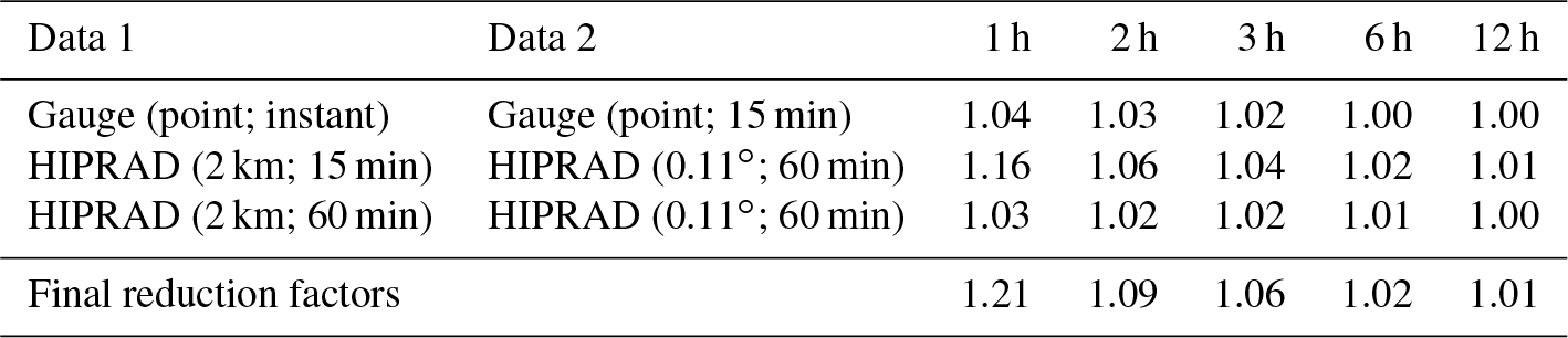
To alleviate this bias, we first derive area and time reduction factors that can be applied to each local data set. We make use of the Swedish radar and gauge-based data set HIPRAD (Berg et al., 2016), as well as 15 min resolution gauge records for the same domain, to derive time and areal reduction factors based on annual maxima for the years 2011–2014; see Table 2. Some grid points, primarily in northern mountainous regions of Sweden, were masked out from the analysis due to unrealistic data. In Olsson et al. (2018b), the intensity reduction for hourly aggregations between near instantaneous and 15 min gauge resolution data was studied with Swedish records and found to be about 4 % at the 1-hourly durations and negligible at a 6 h duration.

HIPRAD is originally available at a 2 km grid and 15 min resolution and was used to compare the reduction factors when both time and space coarsening is considered. When coarsening the time and space resolutions from 2 km and 15 min data to 0.11^∘ and 60 min data, the reduction is about 16 % at an hourly duration and falls to only about 1 % at a 12 h duration. The final conversion factor to go from a near instantaneous point source rain gauge measurement to the 1 h and 0.11^∘ resolution model data becomes the product of the time reduction factor of the gauge data and the space and time reduction factor of HIPRAD, as shown in the last line of Table 2. These factors compare well to previously applied area reduction factors (Sunyer et al., 2016); for example, Wilson (1990) presented a factor 1.279 for hourly precipitation, although at a 24 h duration the factor only decreased to 1.066 indicating a slightly too small factor in our current study. Such differences can be explained by differences in local precipitation climate and is regarded as an inherent uncertainty in this analysis. The factors are applied to the gauge-based local data sets and for the French SHYPRE data set only the space reduction factor for 60 min duration is applied.

Table 2Relative differences in annual maxima averaged over 4 years at different temporal and/or spatial resolutions.

Download Print Version | Download XLSX

4.1 Evaluation

Due to the different methodologies applied in the different national data sets, the evaluation mainly considers the 10-year depths, as this is well within the sample coverage of the data series and is therefore not so sensitive to the choice of method for extreme value calculations, for example, considering the use of AM or POT, or the extreme value distribution applied. The evaluation is therefore qualitative, and we focus only on the main patterns and deviations between the data sets. A general overview of the parameter fits of the extreme value distribution shows minor influence of the driving GCM, but there are differences between the RCMs. At a 12 h duration all RCMs have similar parameter values across Europe (see Figs. S1 and S2 in the Supplement) but at a 1 h duration there are more regional differences, and RACMO22E especially differs with a lower-scale parameter (see Figs. S3 and S4). The differences in the GP parameters indicate differences in the mean and variance of the events in the different RCMs, which might be due to, for example, grid point storms at short durations, as pointed out by Chan et al. (2014b).

When evaluating the DDF statistics, the reduction factors of Table 2 were applied to all national data sets, except for France where the scale gap in time is inherently bridged and only the space scale is adjusted; see Sect. 3. Figure 1 presents the evaluation results for each of the domains with local data. Since only GCM-driven simulations have been analysed, the evaluation is not purely of the RCMs, as would be approximated in reanalysis-driven simulations, but of a mixture between the driving GCM and the RCM response to that forcing. Still, RCM-dependent impacts can be seen in the results. For all domains and most models there is a clear pattern of large dry bias for a 1 h duration, with a clear decrease in bias with longer durations. The main exception from this is the REMO2009 model, which agrees better with observations across all durations. HIRHAM5 also performs better than the RCA4 and RACMO models but has a wetter bias for longer durations. The RACMO22E model produces strong underestimations of extreme intensities, mostly between about −25 % and −50 %.

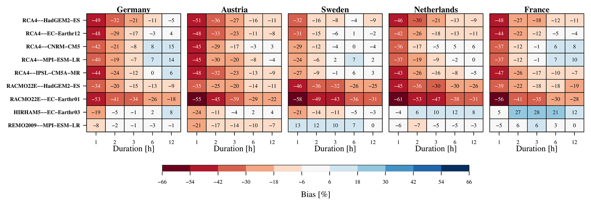
Figure 1Evaluation of model ensemble for selected regions and for the 10-year depths. Gauge-based observations have been adjusted for spatial resolution and time sampling to approximate the statistics of the model resolution and sampling, as explained in the main text. Both colours and numbers indicate the bias.

Download

Observation-based data sets over Germany and France are available as maps, making a visual evaluation possible. Figures 2 and 3 show the 10-year depths for 1 and 12 h durations over Germany, respectively. For both presented durations, the observations show two main high-intensity regions in Germany: one in the pre-Alpine area close to the south-eastern border to Austria and one in the Black forest region oriented in north–south direction in the south-west. Intensities also tend to decrease towards the north. For the hourly duration, all severely underestimate the intensity, except for HIRHAM5 and REMO2009, as also seen in Fig. 1. Here, we see that they also fail in reproducing the spatial pattern, especially for RCA4, which fails to reproduce both the orographic regions in the south or a reversed north–south gradient. Further, the maps for HIRHAM5 and REMO2009 clearly show that although these two simulations perform better in the median intensities in Germany they also fail in reproducing the spatial pattern. The spatial analysis shows that the better performance derived from Fig. 1 is due to generally higher precipitation intensities of the REMO2009 and HIRHAM5 RCMs but not in the right locations. Only when increasing the duration to 12 h do the models start to reproduce the observed spatial patterns; see Fig. 3.

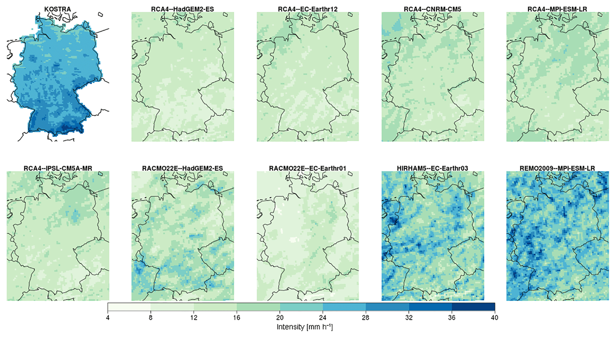
Figure 2Intensity for 10-year return period for 1 h duration of KOSTRA and all models in the RCM ensemble for Germany.

Download

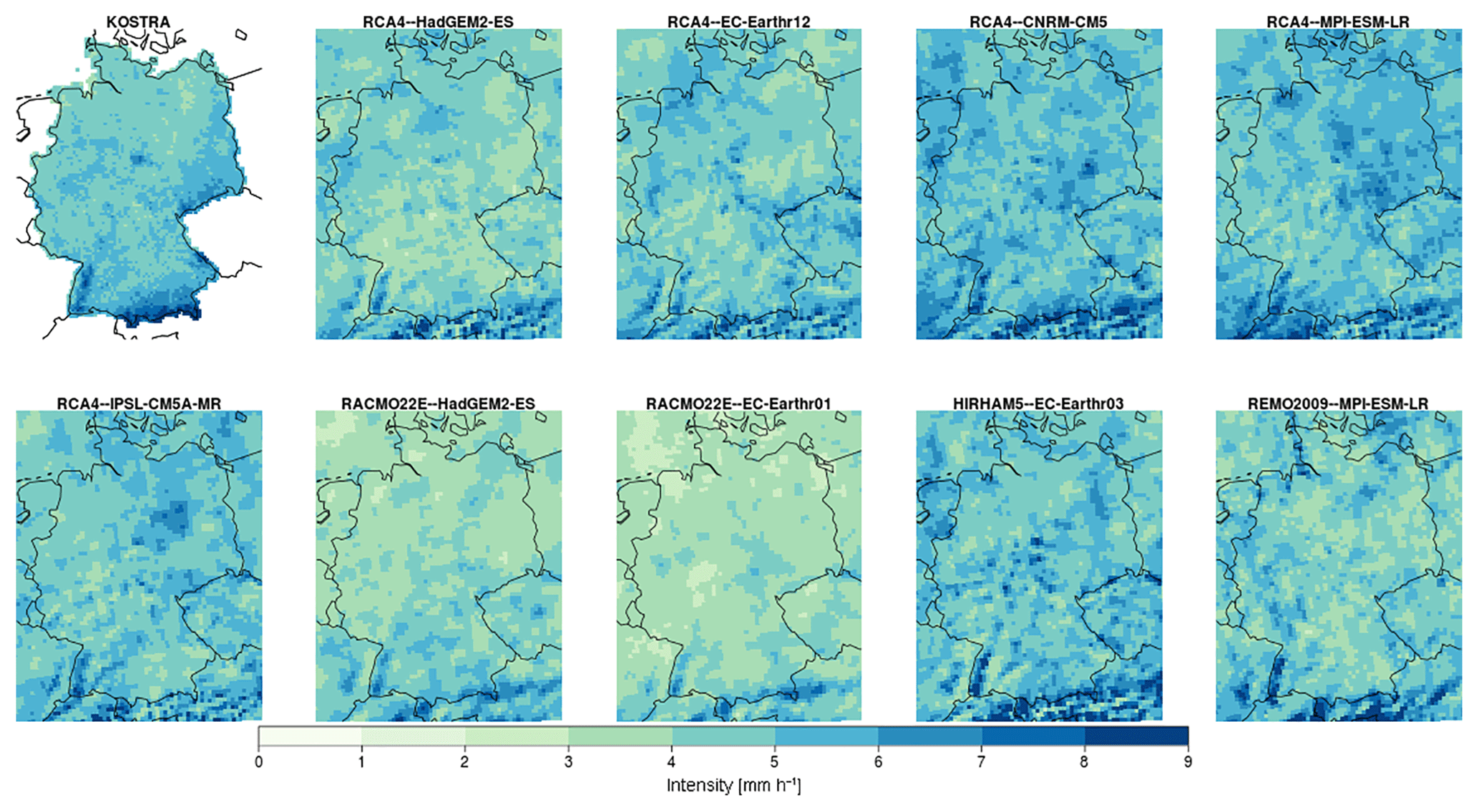
Figure 3Intensity for 10-year return period for 12 h duration of KOSTRA and all models in the RCM ensemble for Germany.

Download

Figures 4 and 5 show similar maps for France and the observation-based data set SHYPRE. SHYPRE shows the highest intensities along the Mediterranean coastline and over the island of Corsica, and intensities decrease gradually towards the north-west. A cautionary note is in place for the comparison of the model analysed summer half-year period to the all-year statistics behind SHYPRE, which can affect conclusions for Mediterranean France with a late autumn convective season. As for Germany, all models but HIRHAM5 and REMO2009 generally underestimate 1-hourly intensities, and the peak intensity region is poorly reproduced in RCA4 and only somewhat better in the RACMO22E simulations. Within the ensemble of each individual RCM, there are variations that are likely due to the driving GCM; however, these variations are small compared to the inter-RCM spread. HIRHAM5 and REMO2009 have clear intensity maxima in the south of France that resemble those of SHYPRE. The 12-hourly durations are better simulated by all models, with the general pattern, at least, being similar to SHYPRE. However, RCA4 and RACMO22E still underestimate intensities, whereas HIRHAM5 and REMO2009 show better agreement regarding intensities.

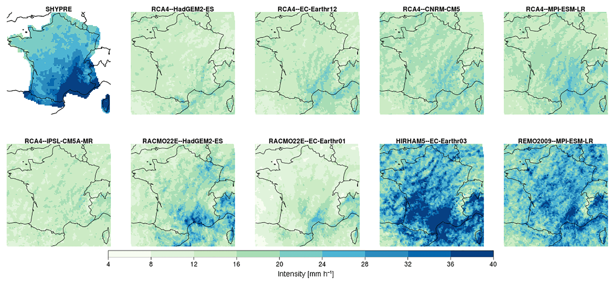
Figure 4Intensity for 10-year return period for 1 h duration of SHYPRE and all models in the RCM ensemble for France.

Download

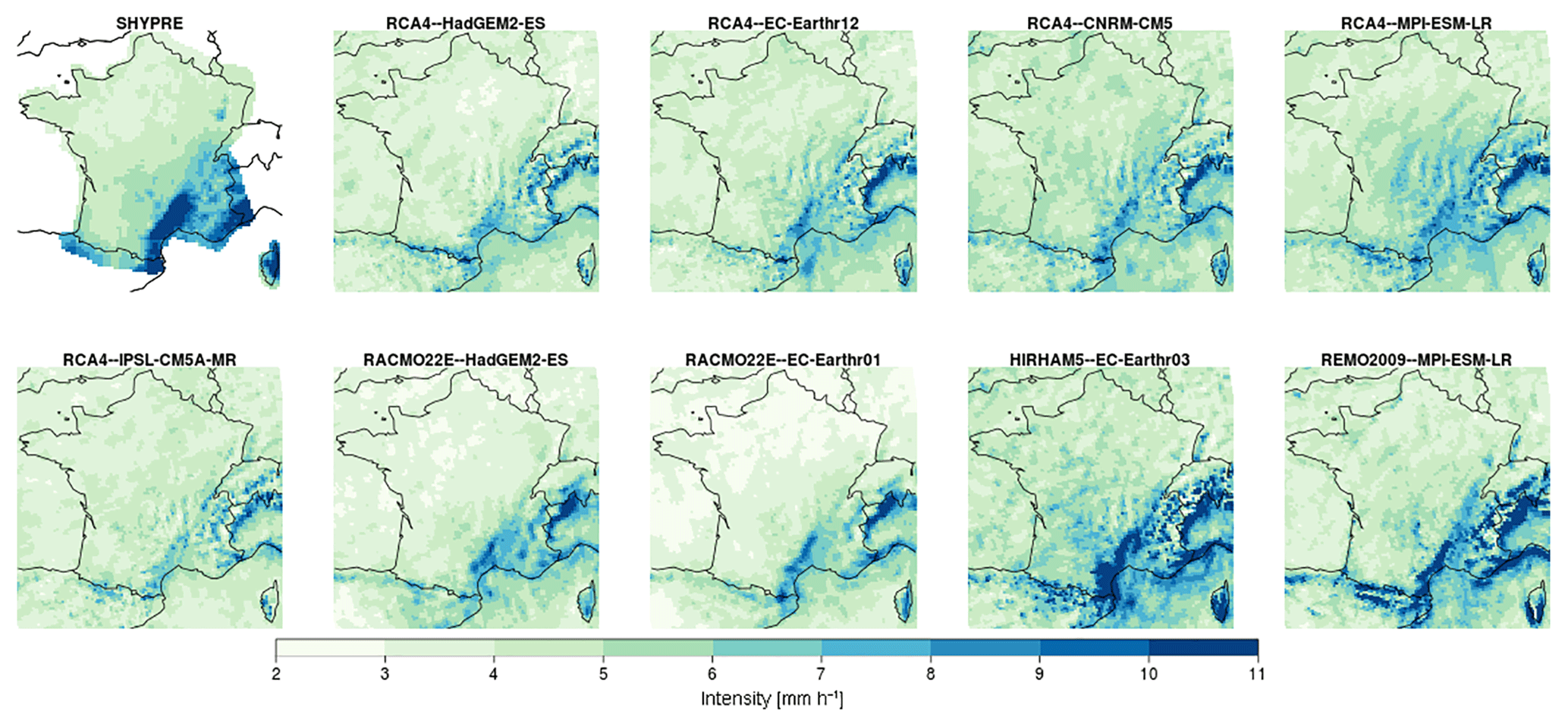
Figure 5Intensity for 10-year return period for 12 h duration of SHYPRE and all models in the RCM ensemble for France.

Download

To complement the evaluation with a pan-European view of modelled extreme intensities, Figs. 6 and 7 show the 10-year depths for 1 and 12 h durations, respectively. At a 1 h duration, all models share a similar structure of higher intensities over the ocean west of France and the Iberian Peninsula and along the northern Mediterranean coastline, although the magnitude differs between the models. The different RCA4 simulations show that the driving GCM has some impact on the pattern across Europe. For example, HadGEM2-ES produces less intense rainfall in southern France, where the MPI-ESM-LR-driven simulation has generally more intense rainfall. However, the driving GCM seems to have less influence than the RCM. At a 12 h duration, the general patterns across Europe converge across all GCM–RCM combinations, although with differences in overall intensities; see Fig. 7. However, it is unclear from this study whether the pattern is correct or not, since observations are lacking. Earlier studies have indicated that the peak of the events is underestimated by the parameterized 0.11^∘ simulations (Kendon et al., 2014), but the large bias in the 1 h durations might also indicate that small concentrated events are missing from the parameterized simulations.

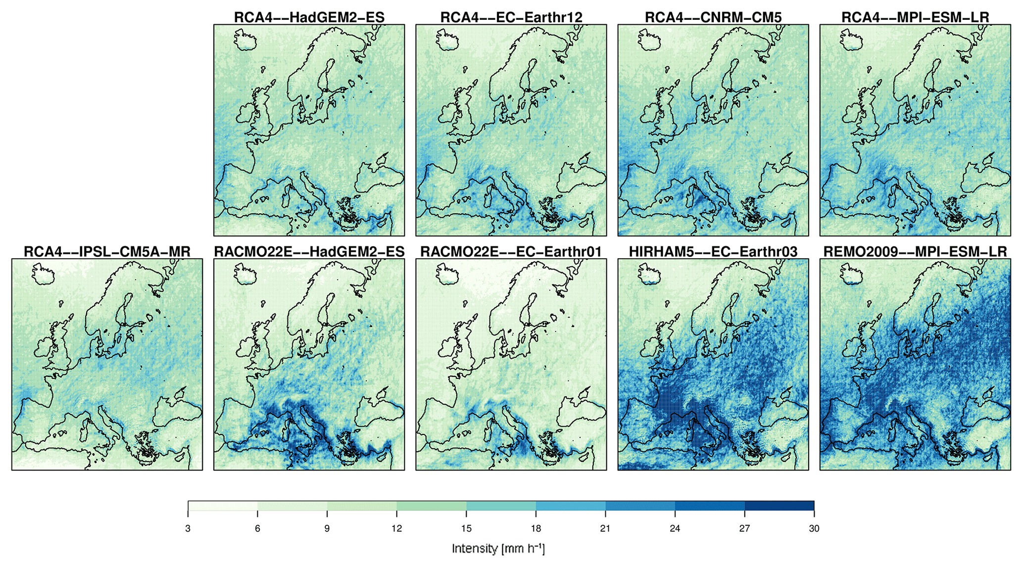
Figure 6Intensity for 10-year return period for a 1 h duration of all models in the RCM ensemble.

Download

Figure 7Intensity for 10-year return period for a 12 h duration of all models in the RCM ensemble.

Download

The general conclusion is that depths for hourly durations are underestimated in the models, which is a likely consequence of model resolution and deficiencies in convective parameterizations. Longer duration events that also tend to have a larger spatial extent are better captured by the grid resolved component of the model simulations, where orographic effects also become more clear in the spatial patterns, in agreement with observations.

4.2 Future projections

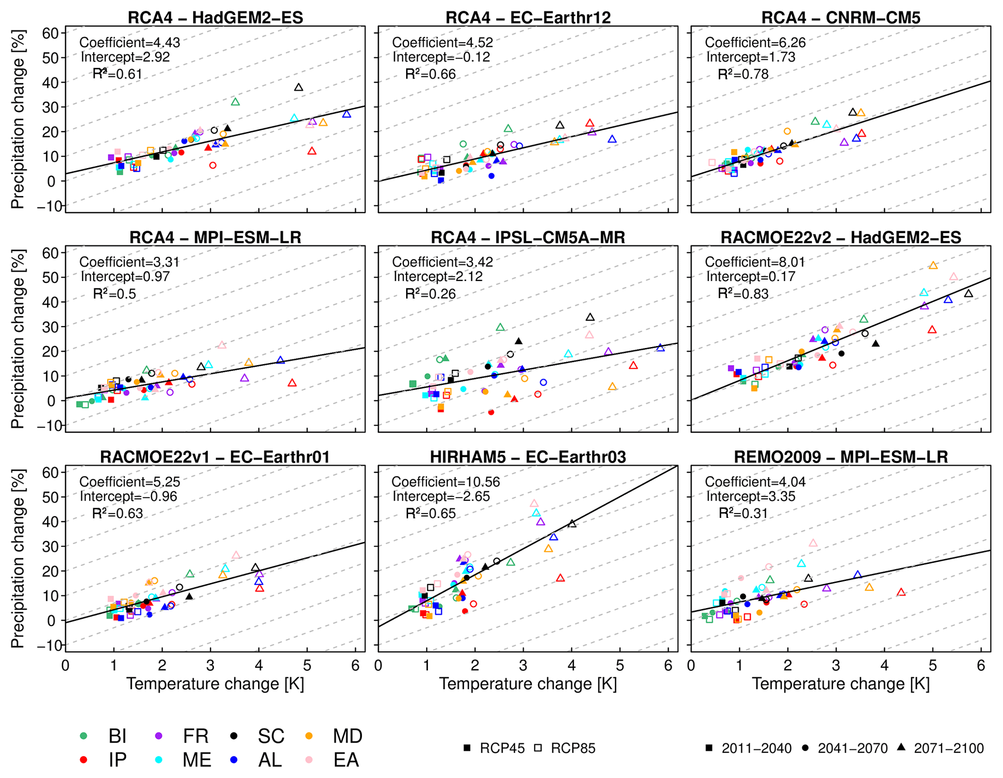
Figure 8Scatterplot of the relative change in 10-year 12 h depths against summertime mean temperature change between future and historical time periods, for different subregions, emission scenarios, and time periods according to the legend. Each panel shows the result for different RCM–GCM combinations. Linear fits to all data are presented in each panel, along with slope and intercept coefficients, as well as the R² value of the fit. CC-rate changes of 7 % K⁻¹ are shown as grey lines in the plots.

Download

The performance of the RCMs in reproducing observed patterns for 12 h durations is promising enough to promote further analysis of future projections. We also include shorter durations in the analysis, despite their poor evaluation performance. Here, we investigate the response of extreme precipitation as a function of the local summer half-year (April–September) temperature change in three future time slices: 2011–2040, 2041–2070, and 2071–2100. The use of a fixed number of events, rather than setting a threshold for the POT-analysis, means that the effective threshold changes between the time slices. The thresholds are generally increasing by 15 % to 50 % for all durations when comparing the end-of-century RCP8.5 with the historical period. The analysis is performed at land-points for the so-called PRUDENCE regions (BI = British Isles, IP = Iberian Peninsula, FR = France, ME = Mid-Europe, SC = Scandinavia, AL = Alps, MD = Mediterranean, EA = Eastern Europe; Christensen and Christensen, 2007), and the depths are related to the change in mean temperature for each subregion between the future time slices and the historical reference period 1971–2000.

Figure 8 shows scatterplots of the changes in 10-year depths for precipitation of a 12 h duration, with the change in local summertime temperature for each ensemble member. The relative change in precipitation was calculated by first performing a domain average, and then calculating the change between time periods. First, it is clear that the scatterplots have strong linear trends even when considering different subregions, different time slices, and different emission scenarios. This indicates a strong connection between the change in precipitation extremes and the seasonal temperature. Second, the individual RCMs show large differences in their response depending on the driving GCM, but different RCMs also respond differently to the same GCM. Results for a 1 h duration show larger spread but good linear fit and stronger scaling (see Fig. S5).

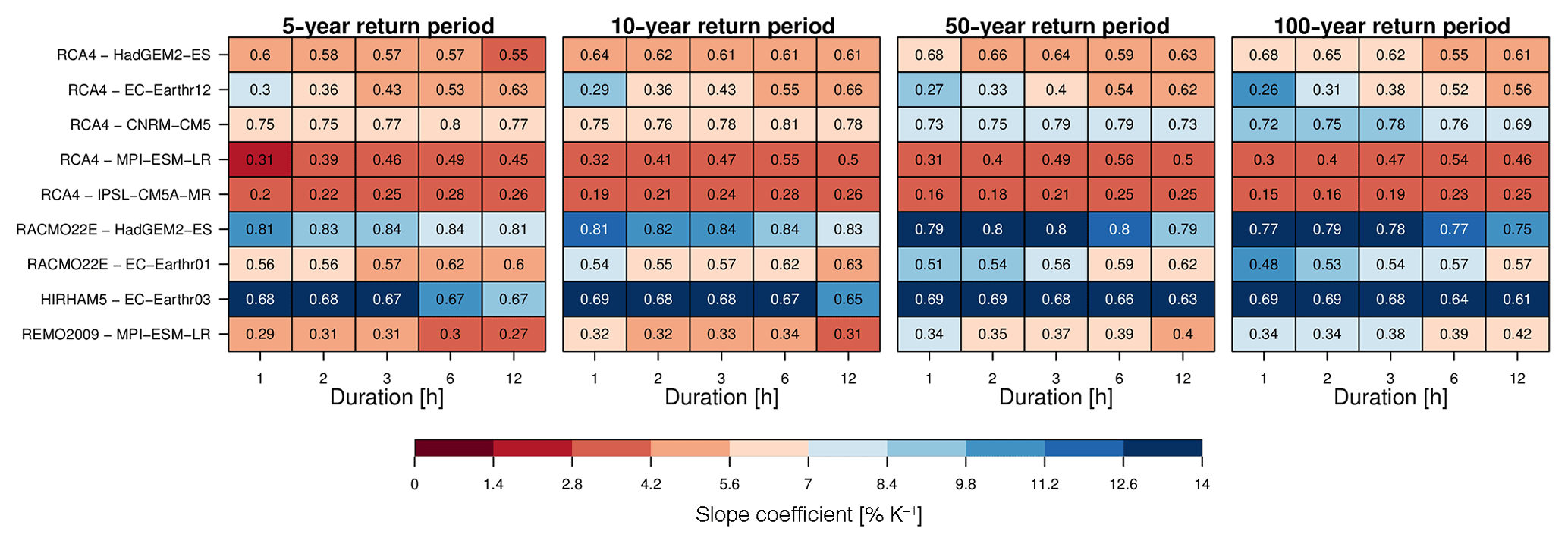
Figure 9Summary of the relative change in precipitation extremes (5, 10, 50, 100-year depths) at various return periods, against summertime temperature change between future and historical time periods for all PRUDENCE regions and RCPs and time slices together. The displayed changes are calculated as the slope coefficient of linear fit, as in Fig. 8. The colour scale is set relative the Clausius–Clapeyron prediction of about 7 % K⁻¹, with red (blue) showing scaling below (above) that rate. The numbers in each box present the R² value for the individual fits as a measure of the goodness-of-fit.

Download

To further investigate the connection between extreme precipitation and seasonal temperature, we perform linear fits for each RCM–GCM combination; see Fig. 8. The results are summarized for all durations and return periods in Fig. 9, with colour coding such that increases beyond the CC-rate are in shades of blue and below the CC-rate are in shades of red. All model combinations show a positive relationship, i.e. increasing slopes, but the slopes vary from about 1 to over 10 % K⁻¹. Most model combinations show stronger scaling for shorter durations (towards the left in each panel) and an increase in scaling with increasing return period (panels toward the right in Fig. 9). The exceptions are the models RCA4-MPI-ESM-LR and RCA4-IPSL-CM5A-MR, which remain at around 3 % K⁻¹ scaling fairly consistently for all durations and return periods. Comparing the influence of the RCM, it is interesting to see that RCA4 driven with EC-Earth scales stronger than with HadGEM2-ES, whereas the opposite is the case for RACMO22E, although the realization of EC-Earth is different, which might have an influence that we cannot quantify in this study. REMO2009-MPI-ESM-LR has slightly stronger scaling than RCA4-MPI-ESM-LR, and HIRHAM5-EC-Earth scales much stronger than the RACMO22E and RCA4 simulations with the same GCM.

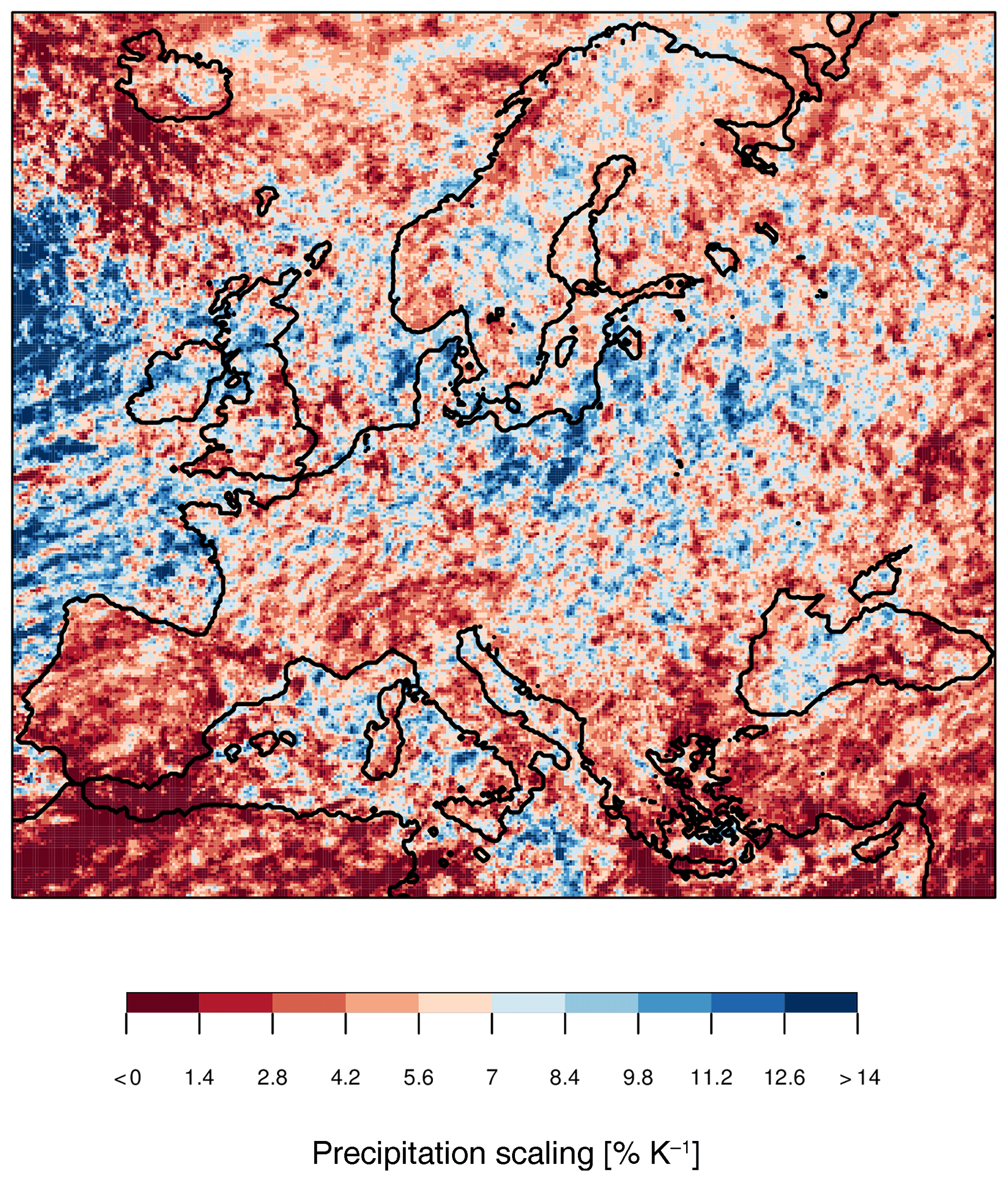
Figure 10Grand ensemble median of scaling factors (% K⁻¹) for 10-year 12 h depths from all models, time slices, and RCPs, calculated separately for each grid point.

Download

Figure 10 shows a grand ensemble median statistic over all models, time slices, and RCPs for each grid point. The weaker than CC temperature scaling in the Mediterranean and Iberian Peninsula land regions is clear and is likely connected to low moisture availability in summer in this region. However, a shift of the main convective season to later in autumn might influence these statistics due to the September cut-off of the investigated summer season. Stronger than CC scaling is seen mainly over water bodies but also in Ireland, the northern UK, and Sweden, which are countries with sufficient atmospheric moisture sources in a future climate as well. However, stronger than CC scaling is also seen in eastern Europe. This feature is prominent in the HIRHAM5 and REMO2009 models but also appears in some other GCM–RCM combinations, such as RACMOE22-HadGEM2-ES and RCA4-CNRM-CM5 (not shown). The regional differences in the scaling seen in Fig. 10 is also apparent on closer inspection of the individual points in Fig. 8.