the Creative Commons Attribution 4.0 License.
the Creative Commons Attribution 4.0 License.
 | 17 Apr 2020
Global-scale benefit–cost analysis of coastal flood adaptation to different flood risk drivers using structural measures
Timothy Tiggeloven
Hans de Moel
Hessel C. Winsemius
Dirk Eilander
Gilles Erkens
Eskedar Gebremedhin
Andres Diaz Loaiza
Samantha Kuzma
Tianyi Luo
Charles Iceland
Arno Bouwman
Jolien van Huijstee
Willem Ligtvoet
Philip J. Ward
Coastal flood hazard and exposure are expected to increase over the course of the 21st century, leading to increased coastal flood risk. In order to limit the increase in future risk, or even reduce coastal flood risk, adaptation is necessary. Here, we present a framework to evaluate the future benefits and costs of structural protection measures at the global scale, which accounts for the influence of different flood risk drivers (namely sea-level rise, subsidence, and socioeconomic change). Globally, we find that the estimated expected annual damage (EAD) increases by a factor of 150 between 2010 and 2080 if we assume that no adaptation takes place. We find that 15 countries account for approximately 90 % of this increase. We then explore four different adaptation objectives and find that they all show high potential in cost-effectively reducing (future) coastal flood risk at the global scale. Attributing the total costs for optimal protection standards, we find that sea-level rise contributes the most to the total costs of adaptation. However, the other drivers also play an important role. The results of this study can be used to highlight potential savings through adaptation at the global scale.
Please read the corrigendum first before continuing.
-
Notice on corrigendum
The requested paper has a corresponding corrigendum published. Please read the corrigendum first before downloading the article.
-
Article
(4047 KB)
-
The requested paper has a corresponding corrigendum published. Please read the corrigendum first before downloading the article.
- Article
(4047 KB) - Corrigendum
-
Supplement
(623 KB) - BibTeX
- EndNote
- Included in Encyclopedia of Geosciences


In recent years, the effects of climate change on coastal flood hazards and its impacts on society have been studied extensively. The Intergovernmental Panel on Climate Change (IPCC) reports that it is likely that we will face a global mean sea-level rise by the end of the 21st century in the range of approximately 0.43–0.84 m compared to 1986–2005 and that impacts on society will be vast (Oppenheimer et al., 2019). According to a recent study by Raftery et al. (2017), it is unlikely that the Paris Agreement's aim of keeping global warming below a 2 ∘C increase by the end of the 21st century will be met. This may lead to changes in storm surges (Tebaldi et al., 2012), extreme sea levels (Vousdoukas et al., 2017), and tides (Pickering et al., 2012). Together, these increases in sea level and a possible change in storminess will lead to increased flood hazards as well as threats to shorelines, wetlands, and coastal development (Ericson et al., 2006; Hinkel et al., 2013). Moreover, flood hazard is expected to increase as a result of subsidence. In many deltas and estuaries, groundwater extraction is a major factor contributing to this subsidence (Hallegatte et al., 2013). During the 20th century, the coasts of Tokyo, Shanghai, and Bangkok subsided by several metres (Nicholls et al., 2008a), and subsidence is expected to continue to affect coastal flood risk in the future (Dixon et al., 2006). Global coastal flood risk is also expected to increase in the future as a result of increasing exposure, due to growth in population and wealth, and economic activities in flood-prone areas (Güneralp et al., 2015; Jongman et al., 2012; Neumann et al., 2015; Pycroft et al., 2016).
Today, on average 10 % of the world population and 13 % of the total urban area in low-elevation coastal zones is located less than 10 m above sea level (McGranahan et al., 2007). In addition, 1.3 % of the global population is estimated to be exposed to a 1-in-100-year flood (Muis et al., 2016). In the coming century, these people and areas are projected to face increases in coastal flood risk (Brown et al., 2018; Hallegatte et al., 2013; Hinkel et al., 2014; Jongman et al., 2012; Merkens et al., 2018; Neumann et al., 2015).
In order to prevent this increase in coastal flood risk, or even to reduce risk below today's levels, adaptation measures are necessary. The importance of climate change adaptation and disaster risk reduction is recognized in several global agreements, such as the Paris Agreement (United Nations Framework Convention on Climate Change, 2015) and the Sendai Framework for Disaster Risk Reduction (United Nations Office for Disaster Risk Reduction, 2015). The Sendai Framework sets specific targets for reducing risk by 2030, such as reducing the direct disaster economic loss in relation to GDP and substantially reducing the number of affected people globally.
Recent studies have shown that adaptation measures hold a large potential for significantly reducing this future flood risk (Diaz, 2016; Hinkel et al., 2014; Lincke and Hinkel, 2018). However, the number of global-scale studies in which the benefits and costs of disaster risk reduction and adaptation are explicitly and spatially accounted for remains limited. Existing studies have assessed the effect of climate change, subsidence, and/or socioeconomic change (Hallegatte et al., 2013; Hinkel et al., 2014; Nicholls et al., 2008b; Vousdoukas et al., 2016) but have not included adaptation objectives or attributed flood risk drivers to adaptation costs. Lincke and Hinkel (2018) assessed the cost-effectiveness of structural protection measures against sea-level rise and population growth using the DIVA model. They found that structural adaptation measures are feasible to invest in for 13 % of the global coastline. However, they did not include subsidence and attribution of drivers in their modelling scheme.
In this paper, we develop a model to evaluate the future benefits and costs of structural adaptation measures at the global scale. We use this to address the limitations of current studies addressed above and thereby extend the current knowledge on the cost-effectiveness of structural adaptation measures in several ways. Firstly, we include human-induced subsidence due to groundwater extraction. Secondly, we assess the benefits and costs of several adaptation objectives. Thirdly, we attribute the costs of adaptation to different drivers (namely sea-level rise, subsidence, and change in exposure).
The overall methodological framework is summarized in Fig. 1 and consists of the following main steps: (1) flood risk estimation, (2) adaptation cost estimation, (3) benefit–cost analysis for four adaptation objectives, and (4) attribution of the total costs to the different drivers. Each of these steps is described in detail in the following subsections. In brief, flood risk is estimated as a function of hazard, exposure, and vulnerability (United Nations Office for Disaster Risk Reduction, 2016). In the risk model, expected annual damage (EAD) is calculated for different scenarios with and without adaptation, with the difference between these two representing the benefits. The costs are calculated by estimating the dimensions of the required dikes (height and length) and multiplying these by their unit costs. Maintenance costs are also included in the cost model. A benefit–cost analysis is performed for four adaptation objectives, and finally the costs of adaptation are attributed to several risk drivers. The methodological steps takes are explained in detail in Ward et al. (2019), on which the following descriptions are based.
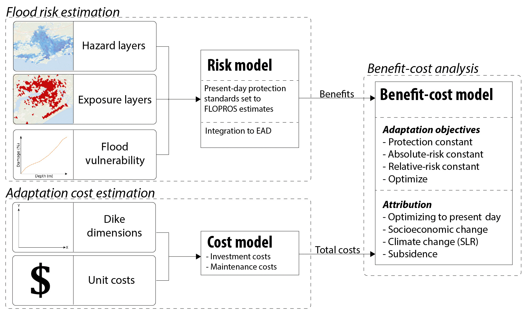
Figure 1Overview of models and data layers for assessing flood risk, costs of adaptation, and attribution of different drivers.
2.1 Flood risk estimation
We use hydrodynamic simulations of tide and surge, and scenarios of regional sea-level rise, as input to a coastal inundation model in order to generate hazard maps for several return periods (2, 5, 10, 25, 50, 100, 250, 500, and 1000 years). These are combined with exposure maps and vulnerability curves (depth–damage functions) in the impact assessment model, using a set-up similar to the GLOFRIS impacts module developed by Ward et al. (2013) and extended for future simulations by Winsemius et al. (2016). The global coastal flood impacts are assessed at a horizontal resolution of and simulated for the different return periods. After calculating the impacts for the different return periods, EAD is calculated by taking the integral of the exceedance probability–impact curve (Meyer et al., 2009). Figure 2 shows the different input layers for the flood risk assessment and benefit–cost analyses (note that different sea-level rise and socioeconomic scenarios are used, and just one is shown in Fig. 2 as example). The following section describes the flood risk simulations in detail.
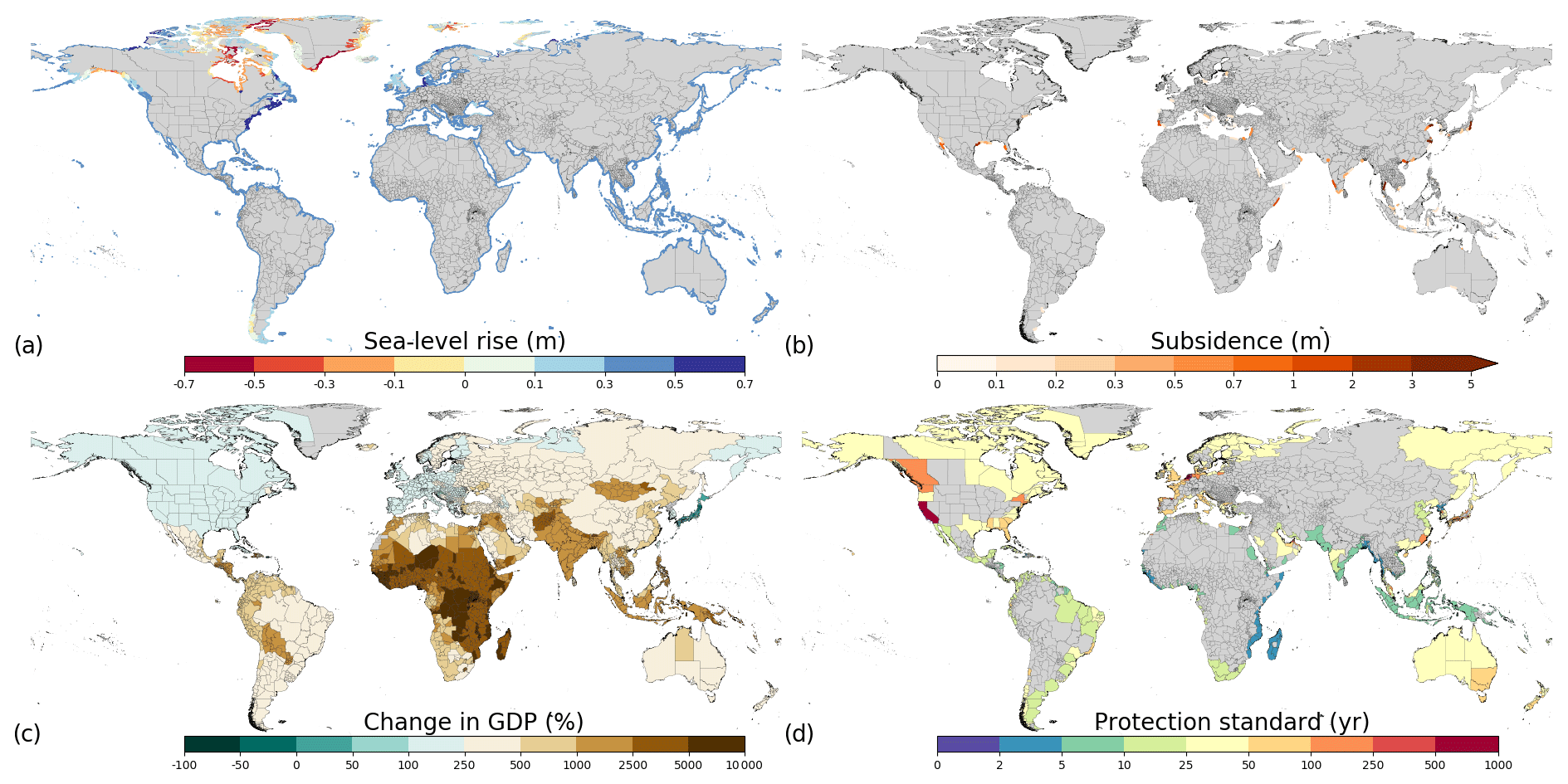
Figure 2Input layers for the benefit–cost analyses: (a) sea-level rise for the RCP4.5 scenario in 2080, (b) subsidence in 2080, (c) change in GDP for the SSP2 scenario in 2080, and (d) current protection standards estimated with the FLOPROS modelling approach.
2.1.1 Flood hazard
Current flood hazard
In order to simulate coastal inundation hazard, we use extreme sea levels from the Global Tide and Surge Reanalysis (GTSR) dataset by Muis et al. (2016) as input to an inundation model. GTSR has been shown to perform well (Muis et al., 2017) for extratropical regions and contains a database of extreme water levels for different return periods based on the Global Tide and Surge Model (GTSM). Surge is simulated using wind and pressure fields from the ERA-Interim reanalysis (Dee et al., 2011), and tide is simulated using the Finite Element Solution 2012 (FES2012) model (Carrère and Lyard, 2003). In this modelling scheme, wind (or surface) waves are not included. As tropical cyclones are poorly represented in the input climate dataset, we use a version of GTSR enriched using a historical storm track archive to represent tropical cyclones. These tropical cyclones were simulated using the IBTrACS (International Best Track Archive for Climate Stewardship) archive, which provides a dataset of historical best tracks. All tracks over the period 1979–2004 are used and converted into wind and pressure fields using the parametric Holland model (Delft3D-WES, 2019) in order to simulate alternative water levels using GTSM. These water levels are combined with the time series of GTSR by using the highest water level at each GTSM cell for each time step. Extreme values are estimated using a Gumbel extreme value distribution fit on the annual extremes.
To calculate overland inundation from near-shore tide and surge levels we used a GIS-based inundation routine, similar to Vafeidis et al. (2019). Extreme sea levels from the nearest GTSR location are projected at the coastline. Then, inundation takes place in areas that are hydrologically connected to the sea for that extreme sea level. The model uses the Multi-Error-Removed Improved-Terrain (MERIT) DEM (Yamazaki et al., 2017) at a resolution as underlying topography. We accommodate three important factors in the inundation routine that are not regularly taken into account in global-scale coastal inundation modelling:
-
We use a resistance factor to simulate the reduction of flooding land inwards, as tides and storm surges have a limited time span. We apply this factor over a Euclidean distance from the nearest coastline point. The resistance factor was set to 0.5 m km−1. Haer et al. (2018) showed the maps to perform well against past flood events in their study in Mexico. Several other studies also use attenuation factors varying between 0.1 and 1.0 m km−1 (Vafeidis et al., 2019).
-
We multiply the resistance factor by a weight, proportional to the amount of permanent water in each cell within the Euclidean pathway towards a land cell under consideration. In this way, grid cells that are marked as land within the terrain model, but in fact represent areas with large amounts of open water, are correctly simulated as cells with low resistance. We estimate fractions of permanent water using a 30-year monthly surface water mask dataset at 30 m resolution, derived from the Landsat archive (Pekel et al., 2016).
-
We apply a spatially varying offset between mean sea level according to the FES2012 model and the datum used by the terrain model MERIT (EGM96) to ensure that the zero datum of our terrain and our extreme sea levels from GTSR are the same.
Future flood hazard
For future hazard simulations we use sea-level changes, to simulate future extreme sea levels, and subsidence estimates due to groundwater extraction to estimate how the terrain may change. Global mean sea-level rise projections for RCP4.5 and RCP8.5 are obtained from the RISES-AM project (Jevrejeva et al., 2014). The sea-level rise for this study is simulated as a range of probabilistic outcomes. For this study, we use the 50th percentile, and to assess the sensitivity of the results, we also use the 5th and 95th percentiles as input for the inundation model. We use gridded datasets of regional sea-level rise estimates developed by Jackson and Jevrejeva (2016). These data were derived by combining spatial patterns of individual sea-level rise contributions in a probabilistic manner. We include sea-level rise in the inundation routine by adding this additional water level to the extreme sea level. Sea-level rise in 2080 for the RCP4.5 scenario and 50th percentile is shown in Fig. 2a. In this simulation, most of the regions will face a sea-level rise between 0.3 and 0.5 m. Close to the poles, sea level may decrease due to a decline in gravitational forces of the melting ice caps.
Subsidence rates are taken from the SUB-CR model by Kooi et al. (2018), which models subsidence using three existing models, namely the hydrological model PCR-GLOBWB integrated with the global MODFLOW groundwater model (de Graaf et al., 2017; Sutanudjaja et al., 2018) and a land subsidence model (Erkens and Sutanudjaja, 2015), focussing on groundwater levels and resulting subsidence. In this approach, subsidence is modelled due to groundwater extraction, which is the dominant factor of human-induced subsidence in many coastal areas (Erkens et al., 2015; Galloway et al., 2016). The effects of subsidence, simulated at the resolution of and spatially interpolated to resolution, are included in the inundation model by adding the subsidence estimates to the MERIT terrain. Subsidence in 2080 is shown in Fig. 2b and reaches up to 5–7 m in regions in China. Unlike sea-level rise, subsidence does not take place along every coastline and is instead projected as a regional phenomenon.
2.1.2 Flood exposure
In our modelling scheme, exposure is represented by maps of built-up area and estimates of maximum damage for three different land use classes in built-up areas. The GLOFRIS model uses current and future built-up area, current and future GDP, and maximum damages on the country level as input. The FLOPROS modelling approach (see Sect. 2.1.5) has current data on built-up area, population, and GDP as input. In the following sections, we describe the exposure data for the current and future simulations.
Current exposure
Current built-up area with a resolution of is taken from the HYDE database (Klein Goldewijk et al., 2010) and later regridded to the resolution. Built-up area refers to all kinds of built-up areas and artificial surfaces. Current maximum economic damages are estimated using the methodology of Huizinga et al. (2017). They used a root function to link GDP per capita to construction costs for each country. To convert construction costs to maximum damages, several adjustments are carried out using the suggested factors by Huizinga et al. (2017) for the different occupancy types. Such factors include depreciation and undamageable parts of buildings. As a proxy for an approximation of percentage area per occupancy type, we set the urban grid cells of the layers from the HYDE database to 75 % residential, 15 % commercial, and 10 % industrial, based on a study by Economidou et al. (2011) and a comparison of European cities' share of occupancy type of the CORINE Land Cover data (EEA, 2016). Following Huizinga et al. (2017), the density of buildings per occupancy types are set to 20 % for residential and 30 % for commercial or industrial.
In order to normalize current risk we use GDP per capita taken from the Shared Socioeconomic Pathways (SSPs) database of IIASA, distributed spatially according to the ORNL LandScan 2010 population count map (Bright et al., 2011). As the total population per country in this map is different to the 2010 population stated in the SSP database, we use a correction factor per country to adjust the population per cell.
Future exposure
Future simulations of built-up area are taken from Winsemius et al. (2016) at a resolution of . Using the method described by Jongman et al. (2012), these simulations were computed using changes in gridded population and urban population for different SSPs derived from the GISMO/IMAGE model (Bouwman et al., 2006). These simulations include five narrative descriptions of future societal development associated with SSP1–5 (O'Neill et al., 2014). Such descriptions include sustainability associated with low challenges (SSP1), middle of the road associated with intermediate challenges (SSP2), regional rivalry associated with high challenges (SSP3), inequality associated with dominance of adaptation challenges (SSP4), and fossil-fuelled development where the mitigation challenges are dominating (SSP5; O'Neill et al., 2017).
To estimate future maximum damages, we scale the current values with the GDP per capita per country from the SSP database. Boundaries of countries are derived from the Global Administrative Areas dataset (GADM, 2012). In order to calculate future risk relative to GDP, future gridded GDP values are taken from Van Huijstee et al. (2018), which uses the national GDP per capita from the SSP database as input.
2.1.3 Flood vulnerability
Vulnerability to flood depth of urban areas is estimated by using different global flood depth–damage functions for each occupancy type that are taken from Huizinga et al. (2017). The resulting damages are represented as a percentage of the maximum damage, reaching maximum damages at a water level depth of 6 m.
2.1.4 Integration to EAD
With the urban damages, calculated for the different return periods, risk is computed and expressed in terms of EAD. We employ a commonly used method in risk assessment to calculate EAD by taking the integral of the exceedance probability–impact (risk) curve (Meyer et al., 2009), which can be written as
where EAD is “risk” per year, D is the urban damage (or impact), θ is the vulnerability, and p denotes the annual probability of non-exceedance (protection standard divided by 1). To fit a protection standard of a coastal region in the risk computation, the risk curve is truncated at the exceedance probability of the protection standard (expressed as a return period). To estimate the definite integral, we use the trapezoidal approximation. As data on protection standards of coastal regions are not available for many regions, we estimate current protection standards for coastal regions using the FLOPROS modelling approach (Scussolini et al., 2016), as described in Sect. 2.1.5.
2.1.5 FLOPROS modelling approach
In order to assess the benefits and costs of adaptation objectives, information on current protection standards is needed. We use the FLOPROS modelling approach (Scussolini et al., 2016) to estimate these protection standards using current exposure data and EAD data from the GLOFRIS model as input. Figure 2d shows the estimated FLOPROS flood protection standards for each coastal sub-national unit. Further information about the FLOPROS estimates together with a validation of the results can be found in the Supplement.
2.1.6 Estimating the benefits of adaptation
In order to calculate the benefits of adaptation, EAD is calculated for every year of the lifetime of the dike for a certain return period and subtracted from the EAD for every year without adaptation. The lifetime of the dike is set to expire in 2100 and the building period is set to 20 years. During this period EAD is assumed to increase linearly. The results are summed to get the total benefits of adaptation.
2.2 Cost estimation
To estimate the costs associated with the different adaptation objectives, we use the same methodology as Ward et al. (2017), which calculates the costs of flood protection by summing the maintenance and investment costs over time for raising dikes to prevent flooding. The following section describes the calculation of costs of adaptation and the adaptation objectives in more detail.
In order to calculate the costs of adaptation, first dike heights need to be calculated. The current dike height calculations are taken from a recent study by van Zelst et al. (2020). Their methodology is to first derive coastal segments and perpendicular coast-normal transects (766 034 transects in total). For each transect, bed levels are constructed, and subsequently, hydrodynamic conditions and wave attenuation are derived. Lastly, the resulting sea water levels are translated into dike heights. The coastlines are derived from OpenStreetMap (OSM) and moved 100 m inwards to smoothen the coastlines and to position the lines at a likely place to establish a dike system. Transects are derived perpendicular to the coastlines for each cell that has a coastline segment. Each transect is described by its slope, ocean bathymetry, foreshore, elevation, and surge levels, among other things. To capture most foreshores, the transects are stretched 4 km inward and seaward. The main source of bed-level data is the Earth Observation-based (USGS Landsat and Copernicus Sentinel 2) high-resolution intertidal elevation map (20 m horizontal and 30–50 cm vertical accuracy) of Calero et al. (2017). As this dataset does not contain data for all bed levels along the transects, the gaps are filled by ocean bathymetry data from GEBCO (30′′, 10 m vertically) and topography data from MERIT (3′′, 2 m vertically). The water levels are derived from the GTSR dataset (Muis et al., 2016) and corresponding wave conditions at different return periods from the ERA-Interim reanalysis (Dee et al., 2011). With a lookup table, consisting of numerical modelling results, the wave attenuation over the foreshore is determined. Due to the unknown direction, incoming waves are assumed to run perpendicular to the coast. Finally, current dike heights with respect to the surge level are calculated with the empirical EuroTop formulations (Pullen et al., 2007) and are based on a standard 1 : 3 dike profile without berms and with a maximum allowed overtopping discharge of 1 L m−2 s−1. This is representative of a low-cost dike. We exclude coastlines where there is no built-up area or no inundation is simulated.
In order to calculate future dike heights, sea-level rise from the RISES-AM project (Jackson and Jevrejeva, 2016) is used in the calculation of the crest heights for different return periods. This is done by adding sea-level rise directly to the crest height. Next to sea-level rise, future dike heights are calculated with subsidence levels (see Sect. 2.1.1.). Subsidence is assumed to take place directly on the dike and therefore computed on the crest height, which is similar for sea-level rise calculations.
The costs of raising dikes are estimated by calculating the total length of dike heightening per grid cell and multiplying by a unit cost set to USD 7 million km m−1 based on reported costs in New Orleans (Bos, 2008). This value of USD 7 million km m−1 is within a reasonable range when compared to various studies (Aerts et al., 2013; Jonkman et al., 2013; Lenk et al., 2017). This includes the costs of investment, groundwork, construction and engineering, property or land acquisition, environmental compensation, and project management. Subsequently, the costs are converted to USD 2005 power purchasing parity (PPP) using GDP deflators from the World Bank and average annual market exchange rates from the European Central Bank for each country. Construction index multipliers, based on civil-engineering construction costs, adjust the construction costs to account for differences between countries (Ward et al., 2010). The lengths of the dikes are estimated using the 766 034 coastline transects. Maintenance costs are represented as percentages of investment costs and are set to 1 % yr−1.
2.3 Benefit–cost analysis
Finally, a benefit–cost analysis is performed by calculating the benefits and costs for adaptation until 2100 for sub-national regions. These regions are defined as the next administrative unit below the national scale in the Global Administrative Areas Database (GADM). The benefits and costs are discounted with a discount rate of 5 % until 2100 (lifespan of investment) and with operation and maintenance (O&M) costs of 1 %. It is assumed that investments are made in 2020 and construction is finished in 2050. During this time period, benefits and costs for investment are assumed to increase linearly. We use the net present value (NPV) shown in Eq. (2) and benefit–cost ratios (BCRs) shown in Eq. (3) as indicators of economic efficiency:
where t denotes the time in years, n the lifespan of the investment, r the discount rate, Bt the benefits per year, Ct costs per year expressed as maintenance costs, and C0 the initial investment costs.
The benefit–cost analysis is carried out for two different sea-level rise scenarios (RCPs) and five different socioeconomic scenarios (SSPs). All the results are shown for two scenario combinations (van Vuuren et al., 2014), namely RCP4.5–SSP2 and RCP8.5–SSP5. The former is used for a “middle-of-the-road” scenario with medium challenges for mitigation and adaptation (Riahi et al., 2017) that can broadly be aligned with the Paris Agreement targets (Tribett et al., 2017), while the latter is used as a “fossil-fuel development” world (Kriegler et al., 2017). Results of the other combinations can be found in the Supplement.
2.3.1 Adaptation objectives
For the benefit–cost analysis, four future investment objectives are explored: (1) the “protection constant”, which keeps protection levels in the future the same as current protection levels, (2) the “absolute-risk constant”, which calculates future protection standards when the absolute value for EAD is kept the same as the current one, (3) the “relative-risk constant”, which calculates future protection standards when EAD as a percentage of GDP is kept the same as the current one, and (4) “optimize”, which calculates future protection standards by maximizing NPV. The future protection standards for the four adaptation objectives are estimated at discrete intervals (2, 5, 10, 25, 50, 100, 250, 500, and 1000 years). The future protection standards when no adaptation takes place are calculated by assuming that dikes are maintained at the current height, but with no additional heightening. In the optimize adaptation objective, only regions with BCRs greater than 1 are included; no adaptation takes place for regions with BCRs less than 1.
2.3.2 Attribution of costs
In order to attribute costs to different drivers, the following method is used. For the optimize adaptation objective, the costs are attributed to four terms: (1) optimization under current conditions (CUR), (2) socioeconomic change (SEC), (3) sea-level rise driven by climate change (SLR), and (4) subsidence driven by groundwater depletion (SUB). The following conceptual equations illustrate the attribution methodology:
Equations (4)–(7) show the attribution calculation, with A being the attribution and NPV the net present value calculated with Eq. (4). The subscripts denote the attribution terms: CUR refers to optimizing in current conditions, SEC refers to socioeconomic change, SLR refers to sea-level rise, and SUB refers to subsidence. ALL refers to when all risk drivers are taken into account. In the subscript between brackets, the baseline protection standard used during the calculation of NPV is indicated. Because the optimize adaptation objective is an optimization and not all regions have optimized their protection standards for the current climate, this last term must be accounted for. The optimization term is the costs of maximizing NPV with current conditions (NPVCUR). Subsequently, the costs for socioeconomic change are computed by taking the difference in costs between NPVCUR and maximizing NPV when only socioeconomic change is taken into account (NPVSEC). To determine the attribution of costs for climate change, the baseline protection is set to the protection standards associated with the NPVSEC term. Subsequently, the costs are estimated by maximizing NPV when both sea-level rise and socioeconomic change are taken into account (NPVSLR). The attribution of subsidence is the same procedure as that with NPVSLR, by swapping the sea-level rise driver with the subsidence driver (NPVSUB). All attributions of costs are expressed in percentages, with reference to maximizing NPV for future conditions (NPVALL), which is the same as the optimize adaptation objective.
In some cases, the percentages of the different drivers do not add up to 100 %. This is the case when absolute dike heights associated with NPVSEC are higher than NPVALL (in other words: adding climate change and subsidence would actually result in lower optimal dike heights in the benefit–cost analysis). In these cases, we set attribution for ATRSEC to 100 % and ATRSLR and ATRSUB to 0 %. Another exception is when optimal protection standards for NPVSEC are higher than NPVSLR or NPVSUB. This occurs when the increase in absolute dike height in the optimization is lower than the effect of sea-level rise or subsidence and results in a lower protection standard. For all other cases, except the two mentioned above, the sum adds to 100 %.
In this section, we first present an assessment of current and future risk without adaptation. Next, we present global benefit–cost analyses for the different adaptation objectives. Then, we present the results of the benefit–cost analyses and the attribution of costs to different drivers at the regional scale. Finally, we assess the sensitivity of the results to changes in various parameters.
3.1 Overview of future flood risk assuming no adaptation
Globally, the estimated EAD increases by a factor of 150 between 2010 and 2080 if we assume that no adaptation takes place in the middle-of-the-road scenario RCP4.5–SSP2. Figure 3 shows the top 15 countries that contribute to this coastal flood risk, in 2010 (Fig. 3a) and 2080 (Fig. 3b) – note the different scales on the x axis. China, Bangladesh, and India have the highest flood risk in absolute terms in 2010. In 2080, these three countries remain in the top four if no adaptation takes place and are joined by the Netherlands. The 15 countries shown account for 89 % of coastal flood risk worldwide in 2010 (USD 19.6 billion per year globally). Although the countries in the top 15 change between current and future assuming no adaptation, the total share of EAD residing in the top 15 countries remains approximately the same: 87 % of global flood risk in 2080 if no adaptation takes place (USD 3 trillion per year globally for RCP4.5–SSP2 and USD 6.8 trillion for RCP8.5–SSP5).
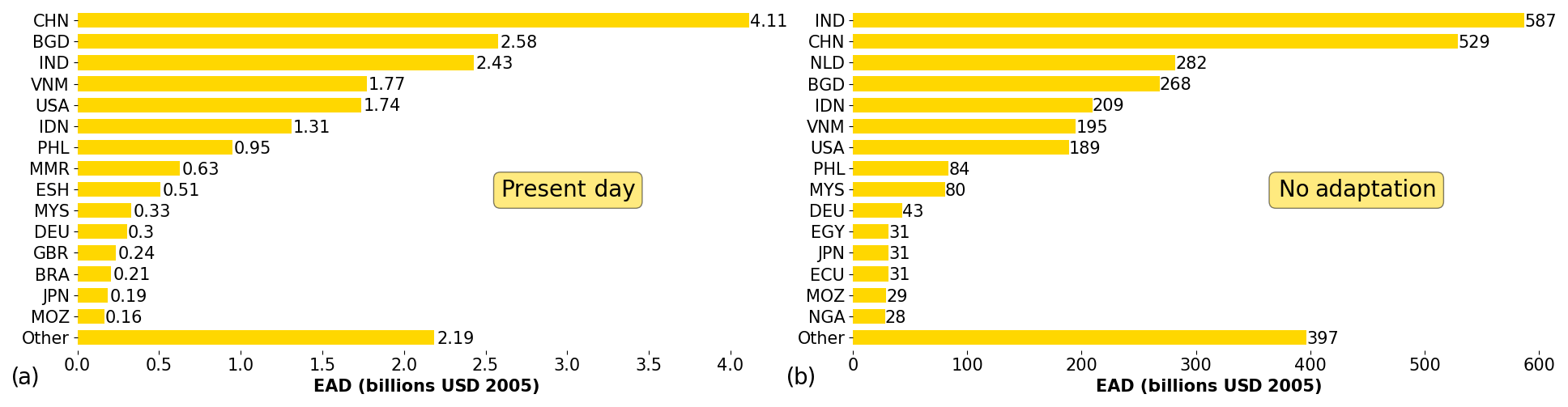
Figure 3Top 15 countries with coastal flood risk in (a) current conditions and (b) 2080 if no adaptation takes place for the scenario RCP4.5–SSP2. Note that the countries and value on the x axis change for each graph. The countries are denoted by ISO 3166-1 alpha-3 codes.
3.2 Global-scale assessment of flood risk under the different adaptation objectives
For all four adaptation objectives, a globally aggregated overview of the benefits, costs, BCR, and NPV is provided in Table 1. All objectives have a positive NPV and BCR higher than 1, indicating that globally the benefits in terms of reduced risk would exceed the investment and maintenance costs. Note that only regions with positive NPV are included for the optimize adaptation objective. The absolute-risk-constant adaptation objective has the lowest BCR, while the optimize adaptation objective has, by definition, the highest BCR. Higher costs and benefits are found for the RCP8.5–SSP5 scenario compared to the RCP4.5–SSP2 scenario, as a result of the larger EAD (and therefore avoided EAD) under this scenario. On average, the costs are ca. 25 % larger in the former, and the benefits roughly double.
Table 1Global overview of benefit–cost analysis for the different adaptation objectives (benefits, costs, and NPV are in USD billion 2005).
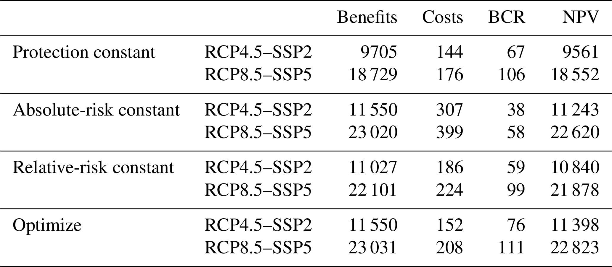
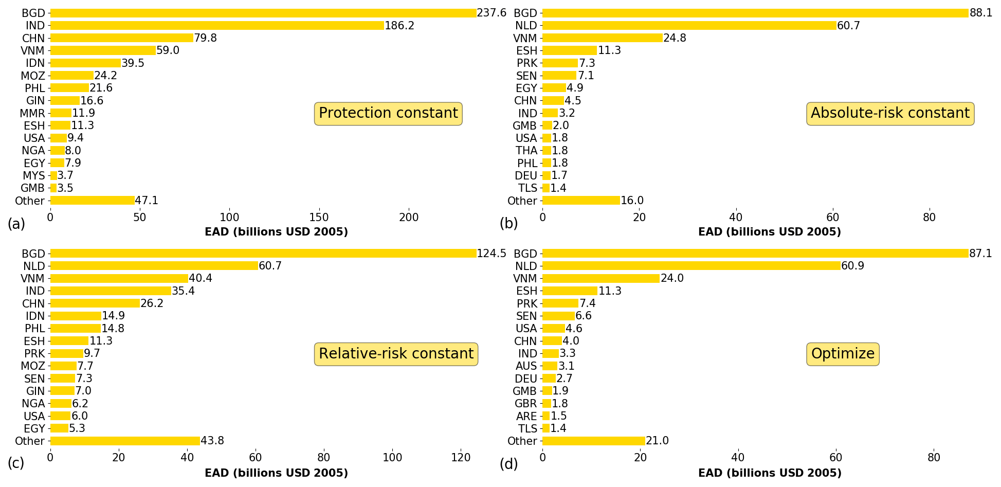
Figure 4Top 15 countries with coastal flood risk in (a) 2080 if protection standards are kept constant, (b) 2080 if absolute risk is kept constant, (c) 2080 if relative risk is kept constant, and (d) 2080 if protection standards are optimized for the scenario RCP4.5–SSP2. Note that the countries and value on the x axis change for each graph. The countries are denoted by ISO 3166-1 alpha-3 codes.
The top 15 countries that contribute the most to coastal flood risk for the four adaptation objectives for RCP4.5–SSP2 in 2080 are shown in Fig. 4. The total share of EAD residing in the top 15 countries remains approximately the same: 94 % of global flood risk in the protection constant adaptation objective (USD 767 billion per year globally), 93 % in the absolute-risk-constant adaptation objective (USD 238 billion per year), 90 % in the relative-risk-constant adaptation objective (USD 421 billion per year), and 91 % in the optimize adaptation objective (USD 242 billion per year globally). Note that EAD can increase in the future for the absolute-risk-constant adaptation objective in certain regions, as we cap protection standards at 1000. The simulated optimal protection standards of the Netherlands are lower than in the protection constant adaptation objective, resulting in a high future EAD of USD 60.9 billion per year. This is because the simulated marginal costs of dike heightening up to a protection standard of 1000 years outweigh the marginal benefits. However, it should be noted that the benefits do exceed the costs up to a 1000-year protection standard and that if this were implemented, the future EAD for the Netherlands in the optimize adaptation objective would therefore be much lower than shown in Fig. 4. Figure S2 in the Supplement shows the top 15 countries for RCP8.5–SSP5.
3.3 Regional-scale assessment of flood risk under the different adaptation objectives
In order to show spatial patterns of the four adaptation objectives, the following results are shown at the sub-national scale in Figs. 5–8. Here, results are shown for RCP4.5–SSP2 only. The same results for RCP8.5–SSP5 can be found in Figs. S2–S5, and the data for all scenario combinations can be found in the Supplement. Although there are some differences between the results for RCP4.5–SSP2 and RCP8.5–SSP5, the overall patterns are very similar.
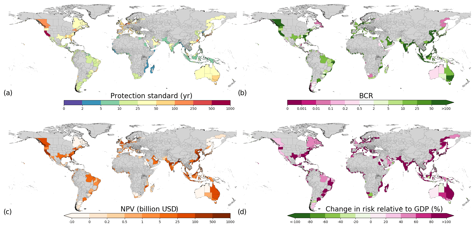
Figure 5Protection constant adaptation objective results of (a) protection standards, (b) BCRs, (c) total NPV, and (d) change in risk relative to GDP for RCP4.5–SSP2. Note that the protection standards (a) are the same as FLOPROS estimates. Regions with no data are indicated in grey.
In the protection constant adaptation objective, the benefits outweigh the costs for the majority of the regions (82 %; 643 of the 784 sub-national regions assessed). Nevertheless, this would still lead to an increase in relative risk (i.e. EAD as a percentage of GDP) in the future for 82 % (641) of the regions assessed. Therefore, only raising dikes to keep up with the current protection standard would lead to a substantial increase in future risk in the majority of the world's regions for scenario RCP4.5–SSP2. Sub-national regions in southern Asia, southeastern Asia, eastern Australia, the eastern and western coast of North America, and parts of Europe have the highest BCR and NPV (Fig. 5). Note that the protection standards (Fig. 5a) are the same as the current protection standards (Fig. 2d).
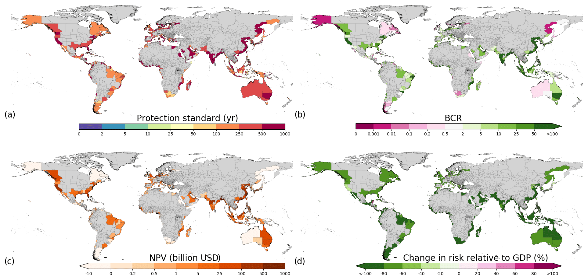
Figure 6Absolute-risk-constant adaptation objective results of (a) protection standards, (b) BCRs, (c) total NPV, and (d) change in risk relative to GDP for RCP4.5–SSP2. Regions with no data are indicated in grey.
In the absolute-risk-constant adaptation objective (Fig. 6), it is clear that dikes would need to be upgraded to have high protection standards (usually between 100 and 1000 years) in order to keep risk constant at current levels. The costs to achieve this are high (globally, more than twice as high as under the protection constant adaptation objective), and therefore a lower number of sub-national regions (79 %; 623) have a positive BCR, although this is still very high. In most sub-national regions, the risk relative to GDP decreases in the future if this adaptation objective is implemented, although 5 % (38) of the sub-national regions show an increase in risk relative to GDP.

Figure 7Relative-risk-constant adaptation objective results of (a) protection standards, (b) BCRs, (c) total NPV, and (d) change in risk relative to GDP for RCP4.5–SSP2. Regions with no data are indicated in grey.
In the relative-risk-constant adaptation objective (Fig. 7), the protection standards required are generally lower than in the absolute-risk-constant adaptation objective. The highest protection standards required are found in eastern Asia and parts of North America. A similar number of sub-national regions have a BCR higher than 1, as is the case for the absolute-risk constant, namely 79 % of the sub-national regions assessed. To keep relative risk constant or absolute risk constant some sub-national regions need to have a future protection standard that is higher than 1000 years (the highest return period assessed in this study). Because of this, the relative change in risk in the relative-risk-constant adaptation objective increases for 5 % (36) of the regions assessed.
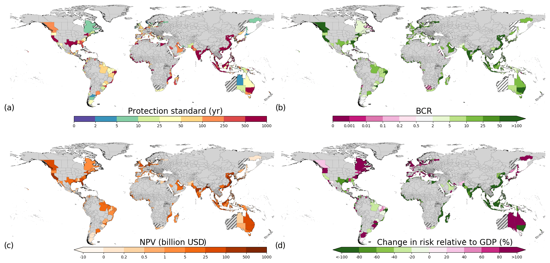
Figure 8Optimize adaptation objective results of (a) optimal protection standards, (b) BCRs, (c) total NPV, and (d) change in risk relative to GDP for RCP4.5–SSP2. Regions where no optimal protection standards are found are indicated with hatched lines, and regions with no data are indicated in grey.
In the optimize adaptation objective (Fig. 8), the highest optimal protection standards are generally found in eastern Asia, southeastern Asia, southern Asia, and the Gulf Coast of the USA. High protection standards are also found in parts of Europe and other parts of the USA, parts of western and eastern Africa, some parts of South America, and southeastern Australia. The highest change in protection standards compared to current is found in southern Asia and southeastern Asia. In most sub-national regions, the benefits exceed the costs when upgrading protection standards (89 %). However, in some sub-national regions the BCR is less than 1 (indicated with hatched lines). The highest values of NPV (Fig. 8c) are found in parts of southern Asia and southeastern Asia, North America, and northwestern Europe. While most sub-national regions show a positive return on investment, there is still an increase in relative risk in 32 % of the sub-national regions assessed, under the optimize adaptation objective. In these cases, it is economically efficient to implement protection measures up to a certain level, yet the economic costs of keeping EAD as a percentage of GDP constant would exceed the avoided damages. Regions where this is especially the case include Europe, North America, South America, Japan, and Australia, as shown in Fig. 8d. Many sub-national regions with decreases in relative risk can be found in southern Asia, southeastern Asia, parts of the Gulf Coast of the USA, New South Wales in Australia, several sub-national regions in Africa, and some parts of South America, among others. In these regions, the increase in risk is generally very high, which means that the costs of investment in protection are lower than the avoided damages relative to GDP. Generally, in these regions, protection standards and/or absolute dike heights increase the most.
In the middle-of-the-road scenario of RCP4.5–SSP2, where the world will face intermediate adaptation and mitigation challenges, we see that most of the sub-national regions assessed would economically benefit from adaptation. We further see that the adaptation objectives differ in changes in relative risk and the level of adaptation that would take place. For instance, in the protection constant adaptation objective we see that although the protection standards stay the same, the relative risk increases for most sub-national regions. This can be explained by the increase in the severity and frequency of the flood hazard due to sea-level rise and subsidence and the increase in exposure of assets due to socioeconomic change. Compared to the optimize adaptation objective, the protection constant adaptation objective under-protects in most sub-national regions. In the absolute-risk-constant adaptation objective we see that relative risk decreases in most sub-national regions while protection standards increase greatly. Due to climate change, socioeconomic change, and subsidence, we see an increase in GDP exposed to flooding. Therefore, protection standards must increase vastly in order to meet the same level of absolute risk. In this adaptation objective, most sub-national regions are over-protected compared to the optimize adaptation objective. In the relative-risk-constant adaptation objective, we see that some sub-national regions are over-protected, while other sub-national regions, for instance in southeastern Asia, are under-protected. The optimize adaptation objective shows the most economically feasible results in terms of maximizing NPV and has the highest BCR in most regions. In the fossil-fuel development scenario of RCP8.5–SSP5, where mitigation will face large and adaptation small challenges (van Vuuren et al., 2014), we see that higher protection standards are required in order to keep risk constant and to maximize NPV (see Figs. S3–S6). The results of the adaptation objectives can be used as a first proxy to indicate the sub-national regions in which adaptation through structural measures may be economically feasible. Moreover, the results indicate regions where adaptation is needed in order to maximize NPV and which objectives under- or over-protect sub-national regions compared to the optimize adaptation objectives. Due to the scope of this study, local-scale models and assessments should be used for the design and implementation of individual adaptation measures.
3.4 Attribution of costs to different drivers of risk
In Fig. 9, we show the percentage of the total costs of the optimize adaptation objective (Fig. 9a) that can be attributed to each of the following risk drivers: climate change (in this case sea-level rise; Fig. 9b), optimizing current protection standards (Fig. 9c), socioeconomic change (Fig. 9d), and subsidence (Fig. 9e). The results are shown for the RCP4.5–SSP2 scenario and only for sub-national regions that have a BCR higher than 1 in the optimize adaptation objective.
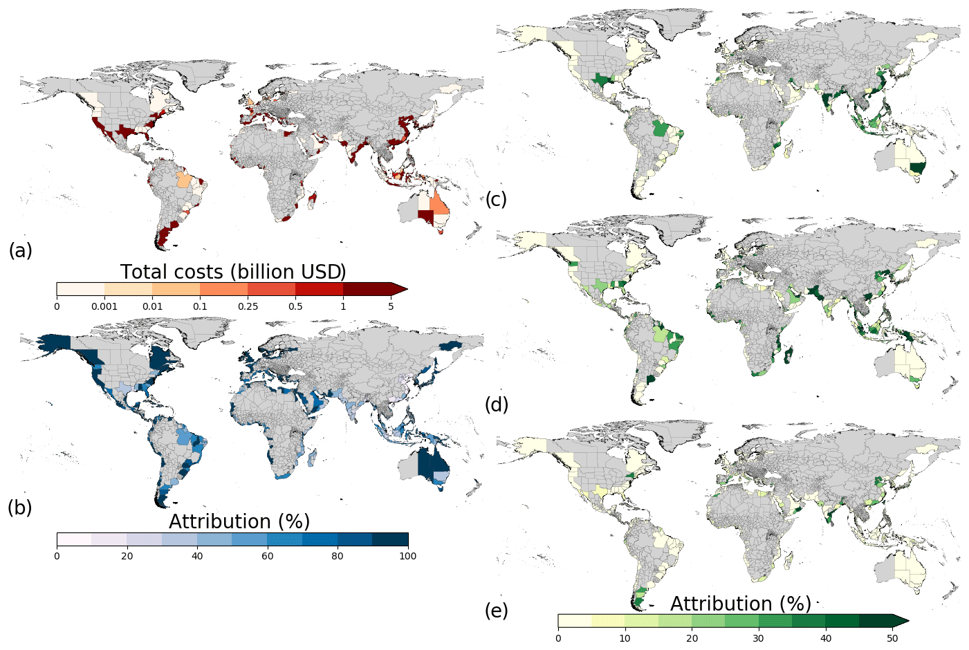
Figure 9Attribution of costs overview for RCP4.5–SSP2, with (a) total costs, (b) attribution of sea-level rise (ATRSLR), (c) attribution of current optimizing (ATRCUR), (d) attribution of socioeconomic change (ATRSEC), and (e) subsidence (ATRSUB). Note that the attribution of SLR is on a different scale, and regions with no data are indicated in grey.
The total costs exceed USD 1 billion for 4 % of the sub-national regions assessed and exceed USD 1 million for 87 %. For most parts of the globe, climate change (in this case sea-level rise) contributes the most to the costs of adaptation, exceeding 50 % of the total costs in 98 % of the sub-national regions (Fig. 9a) and exceeding 90 % of the total costs in 58 % of the sub-national regions. However, the other drivers can also play an important role but are dwarfed in absolute terms by the costs related to sea-level rise. For example, in southern Asia, southeastern Asia, and eastern Africa, optimizing to current conditions and socioeconomic change are important drivers and, in some cases, the most important driver. There are some other regional exceptions where climate change is not the most dominant driver of adaptation costs. Moreover, locally land subsidence due to groundwater extraction can cause huge flood problems and bring large costs in some areas (Dixon et al., 2006; Yin et al., 2013) but are not seen when aggregated to the sub-national regions of this study. However, there are a few regions where subsidence is a more dominant driver (i.e. parts of India, China, Japan, and Taiwan). The results show that climate change is not the most dominant driver in four of the five countries that have the highest share of future EAD if no adaptation takes place (i.e. China, Bangladesh, India, and Indonesia). Generally, the same patterns are found in the attribution results for the RCP8.5–SSP5 scenario, which can be found in the Fig. S7.
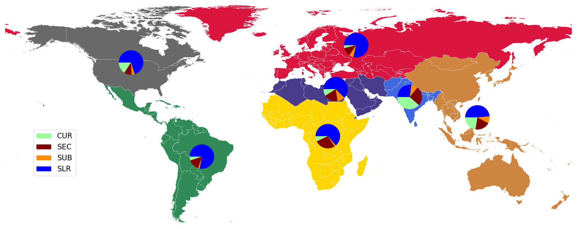
Figure 10Attribution of costs of adaptation for World Bank regions under the optimize adaptation objective and RCP4.5–SSP2 for optimizing to current conditions (CUR), socioeconomic change (SEC), subsidence (SUB), and sea-level rise (SLR).
Figure 10 shows the attribution of the costs for the same scenario and adaptation objective, aggregated to the World Bank regions. In all the regions (except southern Asia), sea-level rise is the most dominant driver, accounting for between 27 % (southern Asia) and 79 % (Europe and central Asia) of the costs of adaptation. The costs of increasing dike height to achieve optimal protection under current conditions are highest in the Global South. This is especially the case for the eastern Asia and the Pacific and southern Asia regions, with values of 22 % and 38 % respectively. The relative contribution of socioeconomic change is largest in eastern Asia and the Pacific, southern Asia, and sub-Saharan Africa, with values of 20 %, 26 %, and 27 % respectively. Of all drivers, subsidence is the least dominant, with values up to 9 % (eastern Asia and Pacific) and 10 % (Middle East and northern Africa). Figure S8 shows the attribution aggregated to the World Bank regions for RCP8.5–SSP5.
3.5 Sensitivity analysis
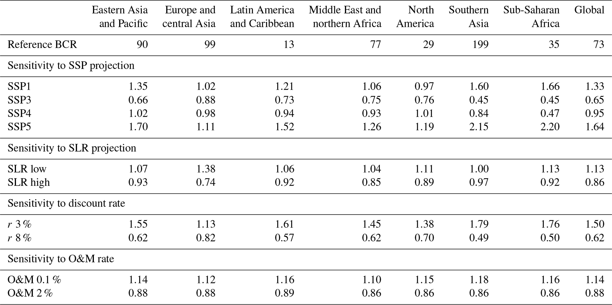
In this section, we show the sensitivity of the results to the use of different SSPs, sea-level rise projections, discount rates, and O&M costs. In Table 2, we show results (of BCR) standardized to a baseline scenario with the following assumptions: RCP4.5, SSP2 (middle of the road), discount rate of 5 %, and O&M of 1 %. We employed a one-at-a-time sensitivity analysis, so for each row in the table only one parameter has changed, and the values shown are standardized by calculating the relative change. All associated BCRs for the standardized values shown in Table 2 are still higher than 1. Globally, BCRs range between 45 and 119 for the different model runs (73 for the reference). At the global scale the BCRs are most sensitive to the use of the different SSPs and discount rates. They cause the largest changes in BCR, with standardized values of 0.44 and 2.17 found in southern Asia and sub-Saharan Africa. Differences in SLR input affect the BCR by a factor of up to 0.38. Europe and central Asia and North America are the least sensitive to the changes in input parameters. The O&M costs show BCRs that are more in line with the reference model run, with higher or lower values up to 0.18.
Table 2Sensitivity analysis of model runs with different input parameters. BCRs are standardized to the model run with RCP4.5–SSP2, discount rate of 5 %, and O&M costs of 1 %. SLR low refers to sea-level rise using the 5th percentile and SLR high to the 95th percentile.
3.6 Comparison to previous studies
Hallegatte et al. (2013) performed a study on future flood risk for 136 major coastal cities. They estimated an EAD of USD 6 billion for current conditions, while in our study we find an EAD of USD 19.6 billion. Our estimates of EAD are higher, which is to be expected given the difference in extent of the studies where we estimate risk for all global coastlines as opposed to 136 major coastal cities in their study. Hallegatte et al. (2013) projected future risk increasing up to USD 60–63 billion if protection standards are kept constant by 2050. In our study we find an EAD of USD 84 billion by 2050 when keeping protection standards constant (RCP4.5–SSP2 scenario). If no adaptation is implemented in 2050, Hallegatte et al. (2013) estimate EAD to be over USD 1 trillion, whereas we find USD 1.1 trillion.
Hinkel et al. (2010) attributed adaptation costs to sea-level rise using dikes for the European Union. They estimated this to be between USD 2.6 billion and 3.5 billion. In our results we find values between USD 12.9 billion and 22.7 billion for the European Union for the scenarios RCP4.5 and RCP8.5 respectively. In a follow-up study, Hinkel et al. (2014) estimate global costs of protecting the coast with dikes. They estimate a range of USD 12–71 billion, while our study estimates the global costs of adaptation for the optimize adaptation objective between USD 152 billion and 208 billion for the RCP4.5–SSP2 and RCP8.5–SSP5 respectively. It should be noted that Hinkel et al. (2010, 2014) use a demand function for safety where dikes are raised following relative sea-level rise and socioeconomic development, while we do not use that function and optimize protection standards by maximizing NPV. This adaptation objective allows dynamic optimization per sub-national region and can result in higher adaptation costs as long as the net benefits increase. Additionally, we use different scenarios than those used in Hinkel et al. (2010, 2014).
Lastly, we compare our results of economic feasibility for sub-national regions and coastlines to the findings of Lincke and Hinkel (2018), in which they found that it is economically feasible to invest in protection for 13 % of the coast globally. Using their method they found a lower share of protected coastline compared to previous studies (Nicholls et al., 2008b; Tol, 2002). In our study, we found that for the optimize adaptation objective, 89 % of the sub-national regions have a BCR higher than 1, indicating that it is economically feasible to implement adaptation in many regions through raising dikes. In our study, the benefit–cost analysis is carried out at the sub-national scale, whereby dikes are only raised on coastal reaches where our transects show there to be potential hazard (inundation) and urban exposure. If we calculate the percentage of the entire global coastline for which this leads to dike heightening in our model with a BCR higher than 1, it amounts to 3.4 % of the global coastline. This is lower than the value in Lincke and Hinkel (2018), but we reason that this difference is a result of the difference in spatial aggregation, where the distance between our transects is 1 km horizontal resolution at the Equator, whilst Lincke and Hinkel (2018) raise dikes along the coast of entire coastal segments, which have lengths ranging from 0.009 to 5213 km, with a mean of 85 km. This can explain why we have a lower percentage of coast that is feasible to protect than Lincke and Hinkel (2018).
3.7 Limitations and future research
While our model scheme does not include dynamic inundation modelling, it does include resistance factors similar to those used by Vafeidis et al. (2019) in order to account for water-level attenuation. It therefore represents an advance to previous studies that have used planar inundation modelling methods (i.e. bathtub models). An improvement could be made by using a dynamic inundation modelling scheme (Vousdoukas et al., 2016) but at the cost of increased computing time. Another improvement can be made by including waves in our inundation modelling, which is found to be an important component in inundation modelling (Vousdoukas et al., 2017). The inundation modelling scheme can be further improved by increasing the resolution from 30′′ to a higher resolution in order to better understand local-scale signals and patterns, since the scale of assessment and resolution of input data have a significant implication on flood risk model results (Wolff et al., 2016). However, we stress that this study aims to understand global flood risk and general patterns at the sub-national scale, and this study can be used as a first proxy, indicating feasibility of adaptation through structural measures, such as dikes.
For this study, results are shown for the scenario RCP4.5–SSP2 and RCP8.5–SSP5 in the Supplement. The range of sea-level rise input values (between the 5th percentile of RCP4.5 and the 95th percentile of RCP8.5) cover a wide range of sea-level rise uncertainty (approximately 0.3–0.7 m at the Equator in the Atlantic Ocean). While in reality the effects of climate change will continue to rise beyond 2100 even if the Paris Agreement is met (Clark et al., 2016), our study examines adaptation objectives until 2100. Results for all combinations of these two RCPs together with all five SSPs can be found in the Supplement.
Several uncertainties exist on the cost calculation side. The first is the monetary value we assumed for the costs of dike heightening. Although we account for differences in costs between countries by using different construction factors and market exchange rates, in reality the costs might differ between regions and may be higher due to local conditions (both physical and socioeconomic). We also use a linear cost function for dike heightening. Using this linear cost function for large-scale studies has been found to be a reasonable assumption according to Lenk et al. (2017).
Another important uncertainty in this study is the current protection standards estimated with the FLOPROS modelling approach, as data on flood protection along the global coastlines are not available. These only provide a first-order estimate of current protection standards per sub-national region. In Fig. S1, a validation of the coastal protection standards estimated with the FLOPROS modelling approach is provided. Values are shown for several locations for which reliable reported estimates of protection standards are available. These reported values are either shown as a range (minimum and maximum reported values) or a single value. Overall, the model performs well. The only location for which the reported values provide a range, and the FLOPROS model lies outside this range, is Durban. However, note that reported values are for the city of Durban, whilst the FLOPROS model value is for the state in which it is located. An improvement to this study could be made by, for instance, mapping flood protections globally by using Earth Observation-based methods.
In this study, several uncertainties exist with assumptions on expected damages per occupancy type. First, we assumed the percentage of occupancy type per grid cell to be the same for all locations, whilst in reality it is spatially heterogeneous, and secondly, we assumed the building density per occupancy type. An improvement could be made by using machine learning to improve accuracy of urban land cover and building types (Hecht et al., 2015; Huang et al., 2018). We also used depth–damage curves per occupancy type, but in reality, these curves also differ between buildings in these occupancy types. To further improve the exposure data of our framework, the Global Human Settlement Layer (Pesaresi et al., 2016) can be used for high-resolution population mapping.
The sub-national regions where no adaptation objective shows a positive BCR should not mean that no adaptation to coastal flood risk should take place. In fact, other adaptation measures (or a combination of multiple measures) besides raising dikes might be more economically feasible in any regions studied, including those with BCRs higher than 1. In this study we only assumed grey infrastructure as adaptation measures, but there are also other measures to reduce flood risk. For instance, the vulnerability can be improved by wet- or dry-proofing buildings (Aerts et al., 2014), or people and assets can be moved to less flood-prone areas in order to reduce the exposure to floods (McLeman and Smit, 2006). Lastly, several local studies show the benefits of nature-based or hybrid adaptation measures (Cheong et al., 2013; Jongman, 2018; Temmerman et al., 2013). Vegetation on the foreshore has a significant role in the breaking of waves (Shepard et al., 2011) and attenuates storm water levels (Zhang et al., 2012). An improvement could be made by including other adaptation measures besides grey infrastructure as adaptation measures.
In this study, four adaptation objectives for reducing (future) coastal flood risk through structural measures have been explored and a benefit–cost analysis has been performed on the sub-national scale for the entire globe. Furthermore, the costs of adaptation have been attributed to different drivers of flood risk: sea-level rise, socioeconomic change, subsidence, and optimizing to current conditions. Globally, we find that EAD increases by a factor of 150 between 2010 and 2080, if we assume that no adaptation takes place, and find that 15 countries account for approximately 90 % of this increase.
We find that all four adaptation objectives show high potential to reduce (future) coastal flood risk at the global scale in a cost-effective manner. The optimize adaptation objective shows the highest NPV (more than USD 11 trillion), with a BCR of 76, while the protection constant adaptation objective shows the lowest NPV (USD 9.5 trillion), with a BCR of 67 for the RCP4.5–SSP2 scenario.
At the regional scale, we show that the adaptation objectives can be achieved with a BCR more than 1 for most of the sub-national regions. This ranges from 89 % for the optimize adaptation objective to 79 % for the absolute-risk-constant adaptation objective. However, we also show that under the optimize adaptation objective, relative risk would still increase compared to current values in 32 % of the sub-national regions assessed.
We assess the sensitivity of the results by performing a one-at-a-time sensitivity analysis to various assumptions and find that, given the uncertainties, implementing structural adaptation measures is a feasible solution for reducing (future) coastal flood risk. Although differences in BCR exist, we show that changes in parameters still result in positive BCRs (between 45 and 120 globally) for the optimize adaptation objective.
Attributing the total costs for the optimize adaptation objective, we find that sea-level rise contributes the most, exceeding 50 % of the total costs in 98 % of the sub-national regions assessed and 90 % of the total costs in 58 % of the sub-national regions. However, the other drivers also play an important role but are dwarfed in absolute terms by the total costs related to the attribution.
The results of this study can be used to highlight potential savings through adaptation at the sub-national scale. Clearly, local-scale models and assessments should be used for the design and implementation of individual adaptation measures, but our results can be used as a first proxy, indicating regions where adaptation through structural measures may be economically feasible. To increase the accessibility of the results to the risk community, the results of this study will be integrated into the Aqueduct Global Flood Analyzer web tool (http://www.wri.org/floods, last access: 14 April 2020).
The results of this study for all RCP and SSP combinations for protection standards, change in risk relative to GDP, B : C ratio, and NPV for all four adaptation objectives are available at: https://doi.org/10.5281/zenodo.3475120 (Tiggeloven, 2019). Figures of the results of RCP8.5–SSP5 combination are available in the Supplement.
The supplement related to this article is available online at: https://doi.org/10.5194/nhess-20-1025-2020-supplement.
TT, PJW, HdM, and HCW conceived the study. All co-authors contributed to the development and design of the methodology. HCW and DE provided coastal inundation layers, and GE provided subsidence rates. AB, JvH, and WL provided data on urban land use and GDP projections. TT analysed the data, with contributions from PJW, HdM, HCW, EG, ADL, SK, and TL. TT prepared the paper, with contributions from all co-authors.
The authors declare that they have no conflict of interest.
This article is part of the special issue “Global- and continental-scale risk assessment for natural hazards: methods and practice”. It is a result of the European Geosciences Union General Assembly 2018, Vienna, Austria, 8–13 April 2018.
The research leading to these results received funding from the Netherlands Organisation for Scientific Research (NWO) in the form of a VIDI grant (grant no. 016.161.324) and the Aqueduct Global Flood Analyzer project, via subsidy 5000002722 from the Netherlands Ministry of Infrastructure and Water Management – the latter project is convened by the World Resources Institute and the Future Water Challenges 2 project, funded by the Netherlands Ministry of Infrastructure and Water Management. We acknowledge funding from the SCOR Corporate Foundation for Science under the project COASTRISK.
This research has been supported by the Netherlands Organisation for Scientific Research (NWO; grant no. 016.161.324), the Netherlands Ministry of Infrastructure and Water Management (grant nos. 5000002722, 31151488), and the SCOR Corporate Foundation for Science under the project COASTRISK.
This paper was edited by Heidi Kreibich and reviewed by Ivan Haigh and Lena Reimann.
Aerts, J. C. J. H., Botzen, W., and De Moel, H.: Cost estimates of flood protection and resilience measures, Ann. N. Y. Acad. Sci., 1294, 39–48, 2013.
Aerts, J. C. J. H., Botzen, W. J. W., Emanuel, K., Lin, N., de Moel, H., and Michel-Kerjan, E. O.: Evaluating flood resilience strategies for coastal megacities, Science, 344, 473–5, https://doi.org/10.1126/science.1248222, 2014.
Bos, A. J.: Optimal safety level for the New Orleans East polder; A preliminary risk analysis, VU Amsterdam, Amsterdam, the Netherlands, 2008.
Bouwman, A. F., Kram, T., and Klein Goldewijk, K.: Integrated modelling of global environmental change: an overview of Image 2.4, available at: https://www.pbl.nl/ (last access: 14 April 2020), 2006.
Bright, E. A., Coleman, P. R., Rose, A. N., and Urban, M. L.: LandScan 2010 High Resolution Global Population Data Set [dataset], available at: http://web.ornl.gov/sci/landscan/ (last access: 14 April 2020), 2011.
Brown, S., Nicholls, R. J., Goodwin, P., Haigh, I. D., Lincke, D., Vafeidis, A. T., and Hinkel, J.: Quantifying Land and People Exposed to Sea-Level Rise with No Mitigation and 1.5 ∘C and 2.0 ∘C Rise in Global Temperatures to Year 2300, Earth's Future, 6, 583–600, https://doi.org/10.1002/2017EF000738, 2018.
Calero, J., Hendriksen, G., Dijkstra, J., and van der Lelij, A.: FAST MI-SAFE platform: Foreshore assessment using space technology, Deltares, Delft, the Netherlands, 2017.
Carrère, L. and Lyard, F.: Modeling the barotropic response of the global ocean to atmospheric wind and pressure forcing – comparisons with observations, Geophys. Res. Lett., 30, 1275, https://doi.org/10.1029/2002GL016473, 2003.
Cheong, S.-M., Silliman, B., Wong, P. P., van Wesenbeeck, B., Kim, C.-K., and Guannel, G.: Coastal adaptation with ecological engineering, Nat. Clim. Chang., 3, 787–791, https://doi.org/10.1038/nclimate1854, 2013.
Clark, P. U., Shakun, J. D., Marcott, S. A., Mix, A. C., Eby, M., Kulp, S., Levermann, A., Milne, G. A., Pfister, P. L., Santer, B. D., Schrag, D. P., Solomon, S., Stocker, T. F., Strauss, B. H., Weaver, A. J., Winkelmann, R., Archer, D., Bard, E., Goldner, A., Lambeck, K., Pierrehumbert, R. T., and Plattner, G.-K.: Consequences of twenty-first-century policy for multi-millennial climate and sea-level change, Nat. Clim. Chang., 6, 360–369, https://doi.org/10.1038/nclimate2923, 2016.
Dee, D. P., Uppala, S. M., Simmons, A. J., Berrisford, P., Poli, P., Kobayashi, S., Andrae, U., Balmaseda, M. A., Balsamo, G., Bauer, P., Bechtold, P., Beljaars, A. C. M., van de Berg, L., Bidlot, J., Bormann, N., Delsol, C., Dragani, R., Fuentes, M., Geer, A. J., Haimberger, L., Healy, S. B., Hersbach, H., Hólm, E. V., Isaksen, L., Kållberg, P., Köhler, M., Matricardi, M., McNally, A. P., Monge-Sanz, B. M., Morcrette, J.-J., Park, B.-K., Peubey, C., de Rosnay, P., Tavolato, C., Thépaut, J.-N., and Vitart, F.: The ERA-Interim reanalysis: configuration and performance of the data assimilation system, Q. J. Roy. Meteor. Soc., 137, 553–597, https://doi.org/10.1002/qj.828, 2011.
de Graaf, I. E. M., van Beek, R. L. P. H., Gleeson, T., Moosdorf, N., Schmitz, O., Sutanudjaja, E. H., and Bierkens, M. F. P.: A global-scale two-layer transient groundwater model: Development and application to groundwater depletion, Adv. Water Resour., 102, 53–67, https://doi.org/10.1016/J.ADVWATRES.2017.01.011, 2017.
Delft3D-WES: Delft3D-WES User Manual, 46, available at: https://content.oss.deltares.nl/delft3d/manuals/Delft3D-WES_User_Manual.pdf (last access: 14 April 2020), 2019.
Diaz, D. B.: Estimating global damages from sea level rise with the Coastal Impact and Adaptation Model (CIAM), Climatic Change, 137, 143–156, https://doi.org/10.1007/s10584-016-1675-4, 2016.
Dixon, T. H., Amelung, F., Ferretti, A., Novali, F., Rocca, F., Dokka, R., Sella, G., Kim, S.-W., Wdowinski, S., and Whitman, D.: Subsidence and flooding in New Orleans, Nature, 441, 587–588, https://doi.org/10.1038/441587a, 2006.
Economidou, M., Atanasiu, B., Despret, C., Maio, J., Nolte, I., and Rapf, O.: Europe's buildings under the microscope. A country-by-country review of the energy performance of buildings, Buildings Performance Institute Europe (BPIE), Brussels, Belgium, 35–36, 2011.
EEA: Corine Land Cover 2012 seamless 100 m raster database (Version 18.5), available at: https://land.copernicus.eu/pan-european/corine-land-cover/clc-2012/ (last access: 14 April 2020), 2016.
Ericson, J. P., Vörösmarty, C. J., Dingman, S. L., Ward, L. G., and Meybeck, M.: Effective sea-level rise and deltas: Causes of change and human dimension implications, Global Planet. Change, 50, 63–82, https://doi.org/10.1016/J.GLOPLACHA.2005.07.004, 2006.
Erkens, G. and Sutanudjaja, E. H.: Towards a global land subsidence map, Proc. IAHS, 372, 83–87, https://doi.org/10.5194/piahs-372-83-2015, 2015.
Erkens, G., Bucx, T., Dam, R., de Lange, G., and Lambert, J.: Sinking coastal cities, Proc. IAHS, 372, 189–198, https://doi.org/10.5194/piahs-372-189-2015, 2015.
GADM: GADM database of Global Administrative Areas, available at: https://gadm.org/data.html (last access: 14 April 2020), 2012.
Galloway, D. L., Erkens, G., Kuniansky, E. L., and Rowland, J. C.: Preface: Land subsidence processes, Hydrogeol. J., 24, 547–550, https://doi.org/10.1007/s10040-016-1386-y, 2016.
Güneralp, B., Güneralp, İ., and Liu, Y.: Changing global patterns of urban exposure to flood and drought hazards, Global Environ. Chang., 31, 217–225, https://doi.org/10.1016/J.GLOENVCHA.2015.01.002, 2015.
Haer, T., Botzen, W. J. W., van Roomen, V., Connor, H., Zavala-Hidalgo, J., Eilander, D. M., and Ward, P. J.: Coastal and river flood risk analyses for guiding economically optimal flood adaptation policies: a country-scale study for Mexico, Philos. T. Roy. Soc. A, 376, 20170329, https://doi.org/10.1098/rsta.2017.0329, 2018.
Hallegatte, S., Green, C., Nicholls, R. J., and Corfee-Morlot, J.: Future flood losses in major coastal cities, Nat. Clim. Chang., 3, 802–806, https://doi.org/10.1038/nclimate1979, 2013.
Hecht, R., Meinel, G., and Buchroithner, M.: Automatic identification of building types based on topographic databases – a comparison of different data sources, Int. J. Cartogr., 1, 18–31, https://doi.org/10.1080/23729333.2015.1055644, 2015.
Hinkel, J., Nicholls, R. J., Vafeidis, A. T., Tol, R. S. J., and Avagianou, T.: Assessing risk of and adaptation to sea-level rise in the European Union: an application of DIVA, Mitig. Adapt. Strat. Gl., 15, 703–719, https://doi.org/10.1007/s11027-010-9237-y, 2010.
Hinkel, J., Nicholls, R. J., Tol, R. S. J., Wang, Z. B., Hamilton, J. M., Boot, G., Vafeidis, A. T., McFadden, L., Ganopolski, A., and Klein, R. J. T.: A global analysis of erosion of sandy beaches and sea-level rise: An application of DIVA, Global Planet. Change, 111, 150–158, https://doi.org/10.1016/J.GLOPLACHA.2013.09.002, 2013.
Hinkel, J., Lincke, D., Vafeidis, A. T., Perrette, M., Nicholls, R. J., Tol, R. S. J., Marzeion, B., Fettweis, X., Ionescu, C., and Levermann, A.: Coastal flood damage and adaptation costs under 21st century sea-level rise, P. Natl. Acad. Sci. USA, 111, 3292–3297, https://doi.org/10.1073/pnas.1222469111, 2014.
Huang, B., Zhao, B., and Song, Y.: Urban land-use mapping using a deep convolutional neural network with high spatial resolution multispectral remote sensing imagery, Remote Sens. Environ., 214, 73–86, https://doi.org/10.1016/J.RSE.2018.04.050, 2018.
Huizinga, J., de Moel, H., and Szewczyk, W.: Global flood depth-damage functions: Methodology and the database with guidelines, JRC Work. Pap., JRC105688, Joint Research Centre, Seville, Spain, 2017.
Jackson, L. P. and Jevrejeva, S.: A probabilistic approach to 21st century regional sea-level projections using RCP and High-end scenarios, Global Planet. Change, 146, 179–189, https://doi.org/10.1016/j.gloplacha.2016.10.006, 2016.
Jevrejeva, S., Grinsted, A., and Moore, J. C.: Upper limit for sea level projections by 2100, Environ. Res. Lett., 9, 104008, https://doi.org/10.1088/1748-9326/9/10/104008, 2014.
Jongman, B.: Effective adaptation to rising flood risk, Nat. Commun., 9, 1986, https://doi.org/10.1038/s41467-018-04396-1, 2018.
Jongman, B., Ward, P. J., and Aerts, J. C. J. H.: Global exposure to river and coastal flooding: Long term trends and changes, Global Environ. Chang., 22, 823–835, https://doi.org/10.1016/J.GLOENVCHA.2012.07.004, 2012.
Jonkman, S. N., Hillen, M. M., Nicholls, R. J., Kanning, W., and van Ledden, M.: Costs of Adapting Coastal Defences to Sea-Level Rise – New Estimates and Their Implications, J. Coast. Res., 290, 1212–1226, https://doi.org/10.2112/JCOASTRES-D-12-00230.1, 2013.
Klein Goldewijk, K., Beusen, A., and Janssen, P.: Long-term dynamic modeling of global population and built-up area in a spatially explicit way: HYDE 3.1, Holocene, 20, 565–573, https://doi.org/10.1177/0959683609356587, 2010.
Kooi, H., Bakr, M., de Lange G., den Haan E., and Erkens, G.: A user guide to SUB-CR: A modflow land subsidence and aquifer system compaction package that includes creep, Deltares, available at: http://publications.deltares.nl/11202275_008.pdf (last access: 14 April 2020), 2018.
Kriegler, E., Bauer, N., Popp, A., Humpenöder, F., Leimbach, M., Strefler, J., Baumstark, L., Bodirsky, B. L., Hilaire, J., Klein, D., Mouratiadou, I., Weindl, I., Bertram, C., Dietrich, J.-P., Luderer, G., Pehl, M., Pietzcker, R., Piontek, F., Lotze-Campen, H., Biewald, A., Bonsch, M., Giannousakis, A., Kreidenweis, U., Müller, C., Rolinski, S., Schultes, A., Schwanitz, J., Stevanovic, M., Calvin, K., Emmerling, J., Fujimori, S., and Edenhofer, O.: Fossil-fueled development (SSP5): An energy and resource intensive scenario for the 21st century, Global Environ. Chang., 42, 297–315, https://doi.org/10.1016/J.GLOENVCHA.2016.05.015, 2017.
Lenk, S., Rybski, D., Heidrich, O., Dawson, R. J., and Kropp, J. P.: Costs of sea dikes – regressions and uncertainty estimates, Nat. Hazards Earth Syst. Sci., 17, 765–779, https://doi.org/10.5194/nhess-17-765-2017, 2017.
Lincke, D. and Hinkel, J.: Economically robust protection against 21st century sea-level rise, Global Environ. Chang., 51, 67–73, https://doi.org/10.1016/J.GLOENVCHA.2018.05.003, 2018.
McGranahan, G., Balk, D., and Anderson, B.: The rising tide: assessing the risks of climate change and human settlements in low elevation coastal zones, Environ. Urban., 19, 17–37, https://doi.org/10.1177/0956247807076960, 2007.
McLeman, R. and Smit, B.: Migration as an Adaptation to Climate Change, Climatic Change, 76, 31–53, https://doi.org/10.1007/s10584-005-9000-7, 2006.
Merkens, J.-L., Lincke, D., Hinkel, J., Brown, S., and Vafeidis, A. T.: Regionalisation of population growth projections in coastal exposure analysis, Climatic Change, 151, 413–426, https://doi.org/10.1007/s10584-018-2334-8, 2018.
Meyer, V., Haase, D., and Scheuer, S.: Flood Risk Assessment in European River Basins – Concept, Methods, and Challenges Exemplified at the Mulde River, Integr. Environ. Asses., 5, 17, https://doi.org/10.1897/IEAM_2008-031.1, 2009.
Muis, S., Verlaan, M., Winsemius, H. C., Aerts, J. C. J. H., and Ward, P. J.: A global reanalysis of storm surges and extreme sea levels, Nat. Commun., 7, 11969, https://doi.org/10.1038/ncomms11969, 2016.
Muis, S., Verlaan, M., Nicholls, R. J., Brown, S., Hinkel, J., Lincke, D., Vafeidis, A. T., Scussolini, P., Winsemius, H. C., and Ward, P. J.: A comparison of two global datasets of extreme sea levels and resulting flood exposure, Earth's Future, 5, 379–392, https://doi.org/10.1002/2016EF000430, 2017.
Neumann, B., Vafeidis, A. T., Zimmermann, J., and Nicholls, R. J.: Future Coastal Population Growth and Exposure to Sea-Level Rise and Coastal Flooding – A Global Assessment, PLoS One, 10, e0118571, https://doi.org/10.1371/journal.pone.0118571, 2015.
Nicholls, R. J., Hanson, S., Herweijer, C., and Patmore, N.: Ranking port cities with high exposure and vulnerability to climate extremes, available at: https://www.oecd-ilibrary.org/content/workingpaper/011766488208 (last access: 15 February 2019), 2008a.
Nicholls, R. J., Tol, R. S. J., and Vafeidis, A. T.: Global estimates of the impact of a collapse of the West Antarctic ice sheet: an application of FUND, Climatic Change, 91, 171–191, https://doi.org/10.1007/s10584-008-9424-y, 2008b.
O'Neill, B. C., Kriegler, E., Riahi, K., Ebi, K. L., Hallegatte, S., Carter, T. R., Mathur, R., and van Vuuren, D. P.: A new scenario framework for climate change research: The concept of shared socioeconomic pathways, Climatic Change, 122, 387–400, https://doi.org/10.1007/s10584-013-0905-2, 2014.
O'Neill, B. C., Kriegler, E., Ebi, K. L., Kemp-Benedict, E., Riahi, K., Rothman, D. S., van Ruijven, B. J., van Vuuren, D. P., Birkmann, J., Kok, K., Levy, M., and Solecki, W.: The roads ahead: Narratives for shared socioeconomic pathways describing world futures in the 21st century, Global Environ. Chang., 42, 169–180, https://doi.org/10.1016/j.gloenvcha.2015.01.004, 2017.
Oppenheimer, M., Glavovic, B. C., Hinkel, J., van de Wal, R., Magnan, A. K., Biesbroek, R., Buchanan, M. K., Abe-Ouchi, A., Gupta, K., Pereira, J., Glavovic, B., Hinkel, J., van de Wal, R., Magnan, A., Abd-Elgawad, A., Cai, R., Cifuentes-Jara, M., DeConto, R., Pörtner, H., Roberts, D., Masson-Delmotte, V., Zhai, P., Tignor, M., Poloczanska, E., Mintenbeck, K., Alegría, A., Nicolai, M., Okem, A., Petzold, J., Rama, B., and Weyer, N.: Sea Level Rise and Implications for Low-Lying Islands, Coasts and Communities, in: IPCC Special Report on the Ocean and Cryosphere in a Changing Climate, edited by: Pörtner, H.-O., Roberts, D. C., Masson-Delmotte, V., Zhai, P., Tignor, M., Poloczanska, E., Mintenbeck, K., and Poh Poh Wong, A., IPCC, Geneva, Switzerland, 2019.
Pekel, J.-F., Cottam, A., Gorelick, N., and Belward, A. S.: High-resolution mapping of global surface water and its long-term changes, Nature, 540, 418–422, https://doi.org/10.1038/nature20584, 2016.
Pesaresi, M., Ehrlich, D., Florczyk, A. J., Freire, S., Julea, A., Kemper, T., and Syrris, V.: The global human settlement layer from landsat imagery, in: International Geoscience and Remote Sensing Symposium (IGARSS), 10–15 July 2016, Beijing China, Institute of Electrical and Electronics Engineers Inc., vol. 2016-November, 7276–7279, 2016.
Pickering, M. D., Wells, N. C., Horsburgh, K. J., and Green, J. A. M.: The impact of future sea-level rise on the European Shelf tides, Cont. Shelf Res., 35, 1–15, https://doi.org/10.1016/J.CSR.2011.11.011, 2012.
Pullen, T., Allsop, N. W. H., Bruce, T., Kortenhaus, A., Schüttrumpf, H., and Van der Meer, J. W.: EurOtop, European Overtopping Manual – Wave overtopping of sea defences and related structures: Assessment manual, also Publ. as Spec. Vol. Die Küste, available at: https://repository.tudelft.nl/islandora/object/uuid:b1ba09c3-39ba-4705-8ae3-f3892b0f2410/ (last access: 5 December 2018), 2007.
Pycroft, J., Abrell, J., and Ciscar, J.-C.: The Global Impacts of Extreme Sea-Level Rise: A Comprehensive Economic Assessment, Environ. Resour. Econ., 64, 225–253, https://doi.org/10.1007/s10640-014-9866-9, 2016.
Raftery, A. E., Zimmer, A., Frierson, D. M. W., Startz, R., and Liu, P.: Less than 2 ∘C warming by 2100 unlikely, Nat. Clim. Chang., 7, 637–641, https://doi.org/10.1038/nclimate3352, 2017.
Riahi, K., van Vuuren, D. P., Kriegler, E., Edmonds, J., O'Neill, B. C., Fujimori, S., Bauer, N., Calvin, K., Dellink, R., Fricko, O., Lutz, W., Popp, A., Cuaresma, J. C., KC, S., Leimbach, M., Jiang, L., Kram, T., Rao, S., Emmerling, J., Ebi, K., Hasegawa, T., Havlik, P., Humpenöder, F., Da Silva, L. A., Smith, S., Stehfest, E., Bosetti, V., Eom, J., Gernaat, D., Masui, T., Rogelj, J., Strefler, J., Drouet, L., Krey, V., Luderer, G., Harmsen, M., Takahashi, K., Baumstark, L., Doelman, J. C., Kainuma, M., Klimont, Z., Marangoni, G., Lotze-Campen, H., Obersteiner, M., Tabeau, A., and Tavoni, M.: The Shared Socioeconomic Pathways and their energy, land use, and greenhouse gas emissions implications: An overview, Global Environ. Change, 42, 153–168, https://doi.org/10.1016/J.GLOENVCHA.2016.05.009, 2017.
Scussolini, P., Aerts, J. C. J. H., Jongman, B., Bouwer, L. M., Winsemius, H. C., de Moel, H., and Ward, P. J.: FLOPROS: an evolving global database of flood protection standards, Nat. Hazards Earth Syst. Sci., 16, 1049–1061, https://doi.org/10.5194/nhess-16-1049-2016, 2016.
Shepard, C. C., Crain, C. M., and Beck, M. W.: The Protective Role of Coastal Marshes: A Systematic Review and Meta-analysis, PLoS One, 6, e27374, https://doi.org/10.1371/journal.pone.0027374, 2011.
Sutanudjaja, E. H., van Beek, R., Wanders, N., Wada, Y., Bosmans, J. H. C., Drost, N., van der Ent, R. J., de Graaf, I. E. M., Hoch, J. M., de Jong, K., Karssenberg, D., López López, P., Peßenteiner, S., Schmitz, O., Straatsma, M. W., Vannametee, E., Wisser, D., and Bierkens, M. F. P.: PCR-GLOBWB 2: a 5 arcmin global hydrological and water resources model, Geosci. Model Dev., 11, 2429–2453, https://doi.org/10.5194/gmd-11-2429-2018, 2018.
Tebaldi, C., Strauss, B. H., and Zervas, C. E.: Modelling sea level rise impacts on storm surges along US coasts, Environ. Res. Lett., 7, 014032, https://doi.org/10.1088/1748-9326/7/1/014032, 2012.
Temmerman, S., Meire, P., Bouma, T. J., Herman, P. M. J., Ysebaert, T., and De Vriend, H. J.: Ecosystem-based coastal defence in the face of global change, Nature, 504, 79–83, https://doi.org/10.1038/nature12859, 2013.
Tiggeloven, T.: Benefit-cost analysis of adaptation objectives to coastal flooding at the global scale (Version 1) [Data set], Zenodo, https://doi.org/10.5281/zenodo.3475120, 2019.
Tol, R. S. J.: Estimates of the Damage Costs of Climate Change. Part 1: Benchmark Estimates, Environ. Resour. Econ., 21, 47–73, https://doi.org/10.1023/A:1014500930521, 2002.
Tribett, W. R., Salawitch, R. J., Hope, A. P., Canty, T. P., and Bennett, B. F.: Paris INDCs, Springer, Cham, Switzerland, 115–146, 2017.
United Nations Framework Convention on Climate Change: COP21 Paris agreement, Le Bourget, France, 2015.
United Nations Office for Disaster Risk Reduction: Sendai framework for disaster risk reduction 2015–2030, UNISDR, Geneva, Switzerland, available at: http://www.unisdr.org/we/inform/publications/43291 (last access: 14 April 2020), 2015.
United Nations Office for Disaster Risk Reduction: Report of the open-ended intergovernmental expert working group on indicators and terminology relating to disaster risk reduction, United Nations General Assembly, New York, NY, USA, 41 pp., 2016.
Vafeidis, A. T., Schuerch, M., Wolff, C., Spencer, T., Merkens, J. L., Hinkel, J., Lincke, D., Brown, S., and Nicholls, R. J.: Water-level attenuation in global-scale assessments of exposure to coastal flooding: a sensitivity analysis, Nat. Hazards Earth Syst. Sci., 19, 973–984, https://doi.org/10.5194/nhess-19-973-2019, 2019.
Van Huijstee, J., Van Bemmel, B., Bouwman, A., and Van Rijn, F.: Towards and Urban Preview: Modelling future urban growth with 2UP, Background Report, PBL, Den Haag, the Netherlands, 2018.
van Vuuren, D. P., Kriegler, E., O'Neill, B. C., Ebi, K. L., Riahi, K., Carter, T. R., Edmonds, J., Hallegatte, S., Kram, T., Mathur, R., and Winkler, H.: A new scenario framework for Climate Change Research: scenario matrix architecture, Climatic Change, 122, 373–386, https://doi.org/10.1007/s10584-013-0906-1, 2014.
van Zelst, V. T. M., Dijkstra, J. T., van Wesenbeeck, B. K., Eilander, D., Morris, E. P., Winsemius, H. C., Ward, P. J., and de Vries, M. B.: Cutting the costs of coastal protection: how vegetation reduces global flood hazard, Nat. Commun., in review, 2020.
Vousdoukas, M. I., Voukouvalas, E., Mentaschi, L., Dottori, F., Giardino, A., Bouziotas, D., Bianchi, A., Salamon, P., and Feyen, L.: Developments in large-scale coastal flood hazard mapping, Nat. Hazards Earth Syst. Sci., 16, 1841–1853, https://doi.org/10.5194/nhess-16-1841-2016, 2016.
Vousdoukas, M. I., Mentaschi, L., Voukouvalas, E., Verlaan, M., and Feyen, L.: Extreme sea levels on the rise along Europe's coasts, Earth's Future, 5(3), 304–323, https://doi.org/10.1002/2016EF000505, 2017.
Ward, P. J., Strzepek, K. M., Pauw, W. P., Brander, L. M., Hughes, G. A., and Aerts, J. C. J. H.: Partial costs of global climate change adaptation for the supply of raw industrial and municipal water: a methodology and application, Environ. Res. Lett., 5, 044011, https://doi.org/10.1088/1748-9326/5/4/044011, 2010.
Ward, P. J., Jongman, B., Weiland, F. S., Bouwman, A., Van Beek, R., Bierkens, M. F. P., Ligtvoet, W., and Winsemius, H. C.: Assessing flood risk at the global scale: Model setup, results, and sensitivity, Environ. Res. Lett., 8, 044019, https://doi.org/10.1088/1748-9326/8/4/044019, 2013.
Ward, P. J., Jongman, B., Aerts, J. C. J. H., Bates, P. D., Botzen, W. J. W., DIaz Loaiza, A., Hallegatte, S., Kind, J. M., Kwadijk, J., Scussolini, P., and Winsemius, H. C.: A global framework for future costs and benefits of river-flood protection in urban areas, Nat. Clim. Chang., 7, 642–646, https://doi.org/10.1038/nclimate3350, 2017.
Ward, P. J., Winsemius, H. C., Kuzma, S., Luo, T., Bierkens, M. F. P., Bouwman, A., de Moel, H., Diaz Loaizaa, A., Eilander, D., Englhardt, J., Erkens, G., Gebremedhind, E., Iceland, C., Kooi, H., Ligtvoet, W., Muis, S., Scussolini, P., Sutanudjaja, E. H., van Beek, R., van Bemmel, B., van Huijstee, J., van Rijn, F., van Wesenbeeck, B., Vatvani, D., Verlaan, M., and Tiggeloven, T.: Aqueduct Floods Methodology, Technical Note, World Resources Institute, Washington, D.C., USA, 2019.
Winsemius, H. C., Aerts, J. C. J. H., Van Beek, L. P. H., Bierkens, M. F. P., Bouwman, A., Jongman, B., Kwadijk, J. C. J., Ligtvoet, W., Lucas, P. L., Van Vuuren, D. P., and Ward, P. J.: Global drivers of future river flood risk, Nat. Clim. Chang., 6, 381–385, https://doi.org/10.1038/nclimate2893, 2016.
Wolff, C., Vafeidis, A. T., Lincke, D., Marasmi, C. and Hinkel, J.: Effects of Scale and Input Data on Assessing the Future Impacts of Coastal Flooding: An Application of DIVA for the Emilia-Romagna Coast, Front. Mar. Sci., 3, 41, https://doi.org/10.3389/fmars.2016.00041, 2016.
Yamazaki, D., Ikeshima, D., Tawatari, R., Yamaguchi, T., O'Loughlin, F., Neal, J. C., Sampson, C. C., Kanae, S., and Bates, P. D.: A high-accuracy map of global terrain elevations, Geophys. Res. Lett., 44, 5844–5853, https://doi.org/10.1002/2017GL072874, 2017.
Yin, J., Yu, D., Yin, Z., Wang, J., and Xu, S.: Modelling the combined impacts of sea-level rise and land subsidence on storm tides induced flooding of the Huangpu River in Shanghai, China, Climatic Change, 119, 919–932, https://doi.org/10.1007/s10584-013-0749-9, 2013.
Zhang, K., Liu, H., Li, Y., Xu, H., Shen, J., Rhome, J., and Smith, T. J.: The role of mangroves in attenuating storm surges, Estuar. Coast. Shelf Sci., 102–103, 11–23, https://doi.org/10.1016/J.ECSS.2012.02.021, 2012.
The requested paper has a corresponding corrigendum published. Please read the corrigendum first before downloading the article.
- Article
(4047 KB) - Full-text XML