the Creative Commons Attribution 4.0 License.
the Creative Commons Attribution 4.0 License.
 | 14 May 2020
Classification and susceptibility assessment of debris flow based on a semi-quantitative method combination of the fuzzy C-means algorithm, factor analysis and efficacy coefficient
Zhu Liang
Songling Han
Kaleem Ullah Jan Khan
Yiao Liu
The existence of debris flows not only destroys the facilities but also seriously threatens human lives, especially in scenic areas. Therefore, the classification and susceptibility analysis of debris flow are particularly important. In this paper, 21 debris flow catchments located in Huangsongyu Township, Pinggu District, Beijing, China, were investigated. Besides field investigation, a geographic information system, a global positioning system and remote-sensing technology were applied to determine the characteristics of debris flows. This article introduced a clustering validity index to determine the clustering number, and the fuzzy C-means algorithm and factor analysis method were combined to classify 21 debris flow catchments in the study area. The results were divided into four types: debris flow closely related to scale–topography–human activity, topography–human activity–matter source, scale–matter source–geology and topography–scale–matter source–human activity. Nine major factors screened from the classification result were selected for susceptibility analysis, using both the efficacy coefficient method and the combination weighting. Susceptibility results showed that the susceptibility levels of 2 debris flow catchments were high, 6 were moderate and 13 were low. The assessment results were consistent with the field investigation. Finally, a comprehensive assessment including classification and susceptibility evaluation of debris flow was obtained, which was useful for risk mitigation and land use planning in the study area and provided a reference for the research on related issues in other areas.
Please read the corrigendum first before continuing.
-
Notice on corrigendum
The requested paper has a corresponding corrigendum published. Please read the corrigendum first before downloading the article.
-
Article
(13667 KB)
-
The requested paper has a corresponding corrigendum published. Please read the corrigendum first before downloading the article.
- Article
(13667 KB) - Corrigendum
- BibTeX
- EndNote


Debris flow is a common geological disaster widely distributed across the world. Due to its sudden occurrence, it is often difficult to give real-time warning. Debris flow usually flows at a speed of 2.88–100.8×10¹⁶ h−1 (Rickenmann, 1999; Clague et al., 1985), inflicting severe damage on lives and properties once it occurs. China is one of the worst-affected areas that is prone to natural disasters. According to data, there are nearly 8500 debris flows distributed across 29 provinces, with an area of approximately 4.3 km×106 km (Ni et al., 2016). Every year, nearly 100 counties are directly endangered by debris flow, and hundreds of people lose their lives, resulting in irreparable losses (Kang et al., 2004).
Debris flow susceptibility analysis (DFS), which expresses the likelihood of a debris flow occurring in an area with respect to its geomorphologic characteristics (Blais-Stevens and Behnia, 2016), is very important for mitigating, evaluating and controlling debris flow disasters (Chiou et al., 2015). Physical, empirical and statistical approaches are used to analyse debris flow, which expresses the presumption of a debris flow occurring in an area with respect to its geomorphologic characteristics (Blais-Stevens and Behnia, 2016). Physically based approaches (Carrara et al., 2008; Burton and Bathurst, 1998) are more applicable to analysing physical and mechanical factors in independent catchments. The empirical model belongs to qualitative evaluation and is too subjective to be convincing. Statistical analyses which are usually applied to the research of regional debris flow belong to quantitative evaluation and depend on the completeness and accuracy of data. For a study area with a limited number of debris flows, a semi-quantitative evaluation method is more appropriate. This analysis includes the extraction of evaluation factors, the determination of weight factors and the establishment of an evaluation model. Considering that the influencing factors of debris flow are complex, multiple evaluation indices are generally involved, and linear correlations between different factors further complicate debris flow susceptibility analysis (Benda and Cundy, 1990). However, the unreasonable selection of factors may cause the loss of important information and failure to obtain accurate evaluation results. One way to alleviate these problems is dimension reduction through factor analysis (FA) (Aguilar and West, 2000). Some researchers (Peggy et al., 1991; Shi et al., 2015) have used the principal-component analysis method to conduct effective dimensionality reduction for selected factors and eliminate the correlation between factors. However, the coefficient of the principal component after dimensionality reduction can be positive or negative, which is not ideal for the occurrence of debris flow. Factor analysis, in which the coefficients of the common factors are all positive and the variables are more resolvable by rotation technology, is applied in the current study.
To determine the influence of different factors on debris flow susceptibility, the weights of these factors should be assigned first. The combined weighting method, which has the advantages of subjective and objective weighting methods, was applied to assign factors with logical weights.
The efficiency coefficient method (ECM) is a comprehensive evaluation method based on multiple factors and is suitable for complex research objects, such as debris flow. The factors can be converted into measurable scores through the appropriate function and objectively reflect the situation of the evaluation object in the case of a large difference in the factor value. This research primarily focuses on the method, which is applied to the debris flow susceptibility evaluation based on the results of the weight analysis.
Debris flow classification plays a direct guiding role in disaster prevention and mitigation, and mature classification methods have been developed (Iverson et al., 1997; Brayshaw and Hassan, 2009). However, a single classification standard cannot fully and accurately reflect the comprehensive characteristics of debris flow ditches, and based on different classification criteria, the same debris flow will belong to different types at the same time. The fuzzy C-means (FCM) method, which is applicable to a wide variety of geostatistical data analyses (Bezdek, 1981), was applied to classify debris flow in this paper. Considering that the main influencing factors of different types of debris flow are also different, FA was carried out for each category to obtain major factors to define each type of debris flow.
In recent years, with the improvement of computer performance and the advanced features in geographic information systems (GISs), global positioning systems (GPSs) and remote-sensing (RS) techniques, these systems, also known as “3S technology”, have become very effective and useful especially to debris flow research (Gómez and Kavzoglu, 2004; Glade, 2005; Conway et al., 2010). In particular, the application of GISs has greatly improved the ability of spatial data processing and analysis, such as slope direction analysis and flow direction calculation (Mhaske and Choudhury, 2010; Xu et al., 2013; Kritikos and Davies, 2015). Therefore, the FA, FCM and ECM were used to classify and evaluate the susceptibility of debris flow in the current study, being combined with 3S technology and field investigation.
The research area is located around several scenic spots in Huangsongyu Township, Pinggu District, Beijing. The village covers an area of 12.83 km2, including 732 households, or a total of 2043 people. The Shilin Gorge is the core scenic area of Huangsongyu Geopark, attracting a large number of tourists year-round. The geographical location of the study area and 21 debris flow catchments are shown in Fig. 2. During our field investigation, some scenic spots have been closed down due to the threat of falling rocks, floods and debris flow, which are shown in Fig. 3. Figures 4 and 5 show the situation of the other two scenic spots. Considering the sudden and rapid occurrence of debris flow and the large number of tourists and surrounding villagers in the scenic area, it is necessary to assess the susceptibility of debris flow.
The study area is located in the northwest of the North China Plain, which belongs to the Yanshan. Surrounded by high terrain, the central part is flat, the highest elevation of the territory is 1188 m and the lowest elevation is 174 m. The Yanshanian and Indosinian periods in the study area were characterised by strong tectonic activity, which resulted in a series of large fold and fault structures. Due to long-term geological processes, the structure in the area is relatively complex. But the strata are relatively simple, except for a few Archean metamorphic rocks; the exposed strata are middle Proterozoic sedimentary strata and Quaternary sediments. The main lithology of the Archean age (Ar) is amphibious plagiarise gneiss and biotite gneiss. The Great Wall System (Ch) is the broadest strata in this area, and the main lithology is dark gray ferric dolomite, silicalite micritic dolomite and dolomite sandstone. The main lithology of the Jixian System (Jx) is dolomite. The Quaternary System (Q) is dominated by sand, gravel and clay of residual and diluvial facies. The non-developed lithology of magmatite is mainly granite and quartz diorite.
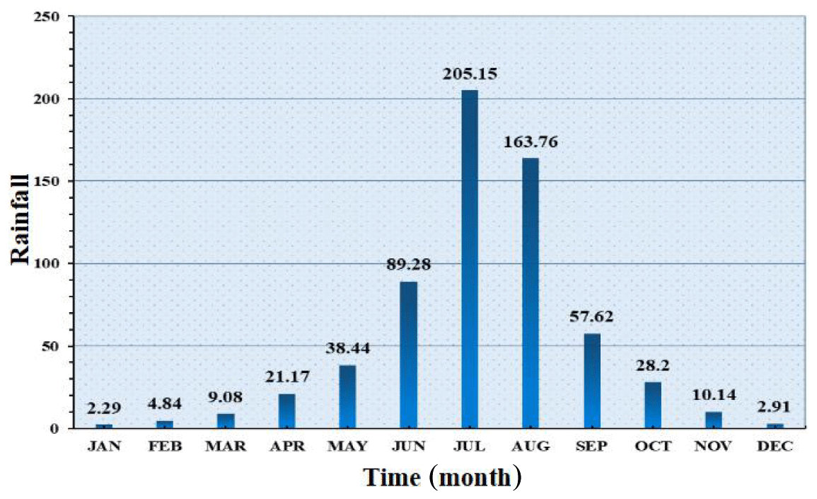
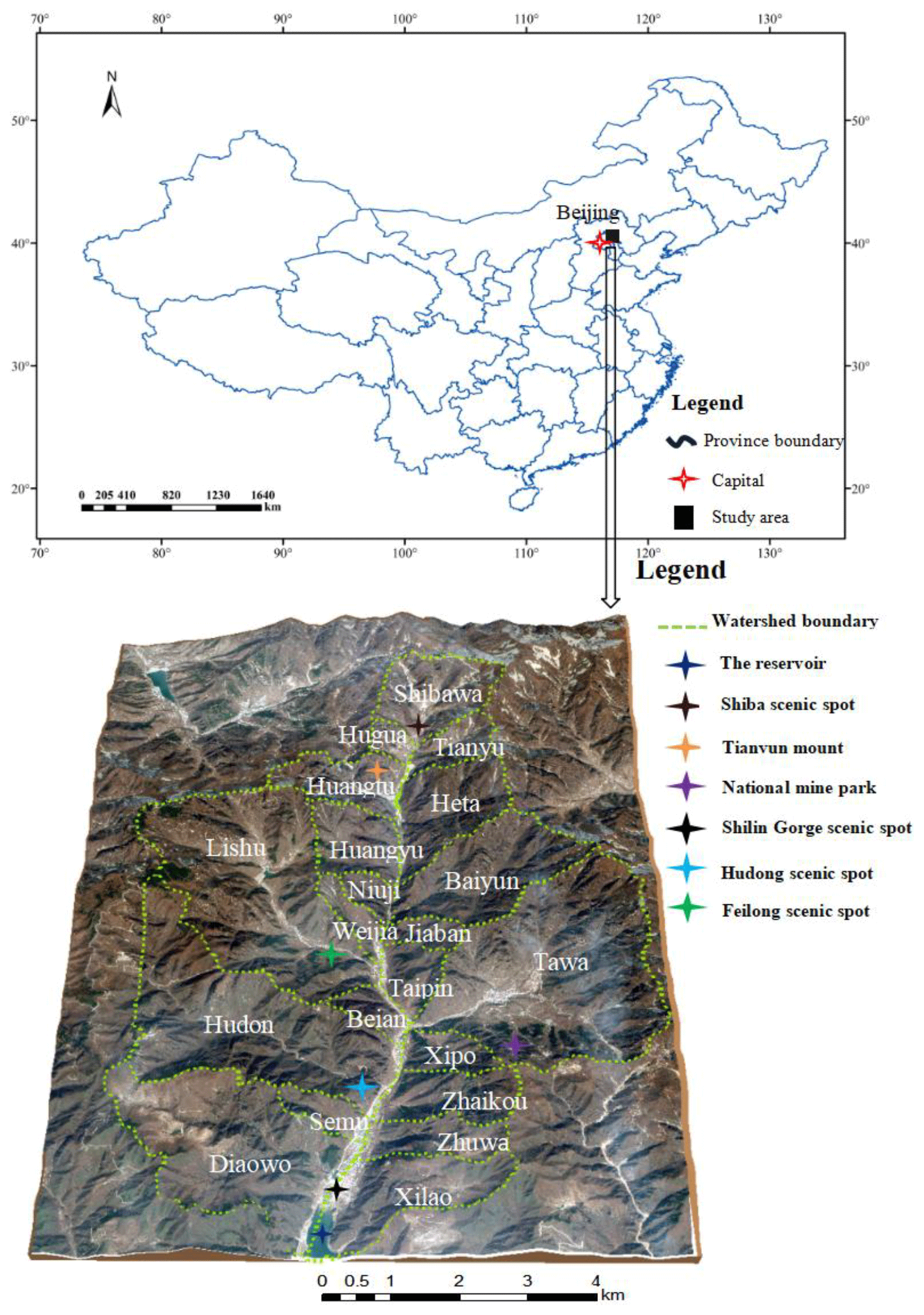
Figure 2Geographical positions of the Huangsongyu scenic region and the investigated 21 debris flow catchments.
The study area is characterised by a northern temperate continental climate, with four distinct seasons and large annual temperature variation. The coldest average January temperature is 6–8 ∘C, and the hottest July average temperature is 21.6 ∘C. The annual precipitation is about 639.5 mm, and the average monthly rainfall (1959–2017) is shown in Fig. 1. Precipitation is concentrated in the summer, accounting for 74.9 % of the annual precipitation, which is generally concentrated in late July and early August, promoting debris flow.
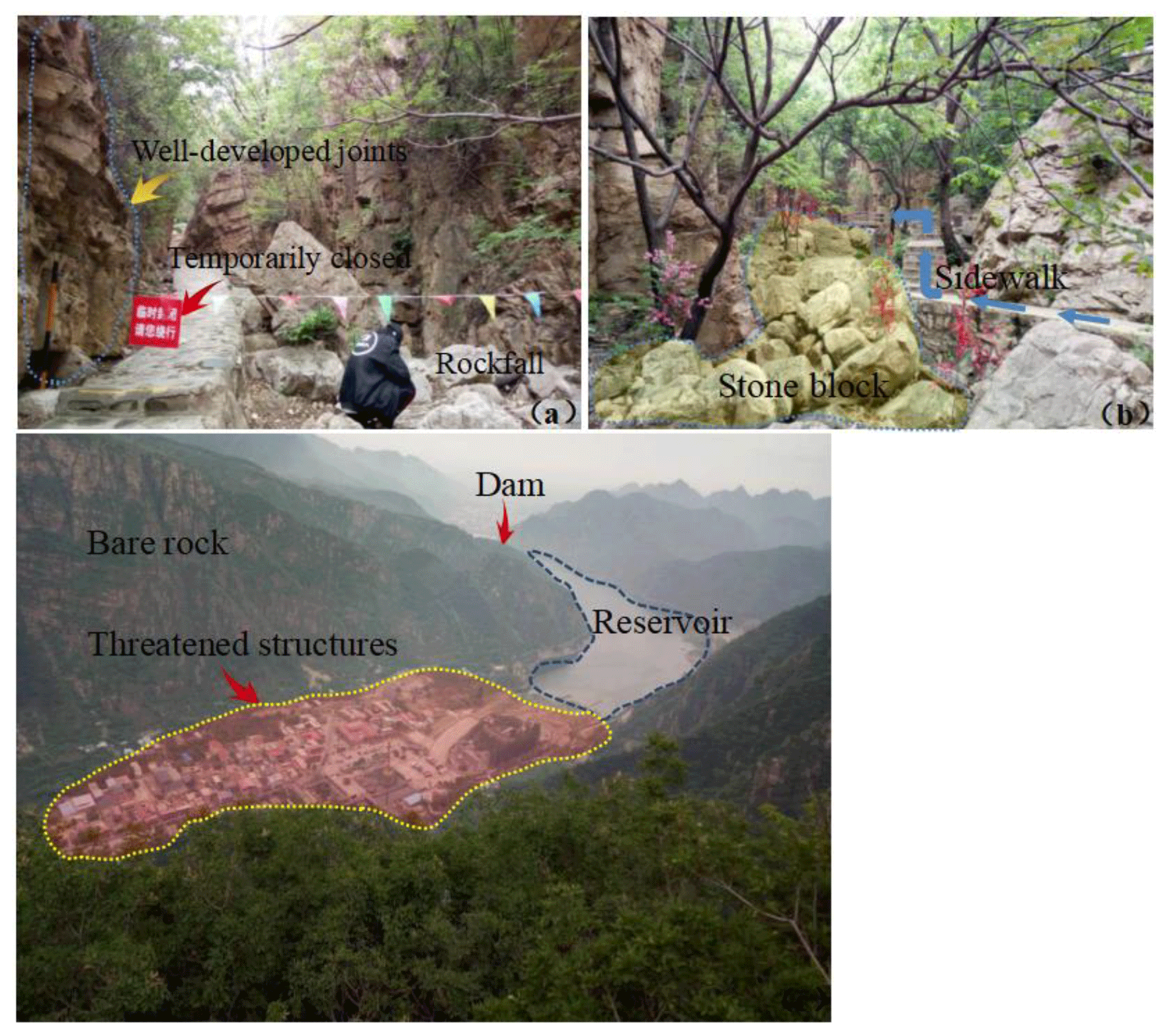
Figure 3Shilin Gorge scenic spot. (a) Some scenic spots have been closed, and (b) the scenic area was heavily blocked by rockfill. (c) Structures threatened by debris flow.
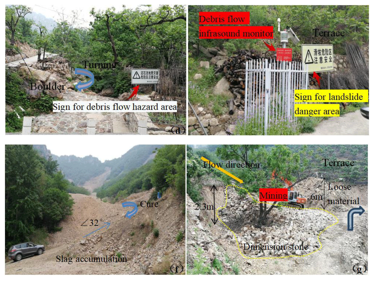
Figure 4Huangsongyu National Mining Park. d is debris flow hazard area, e is debris flow monitoring instrument, f is loose slag accumulated in formation area and g is excavator mining.
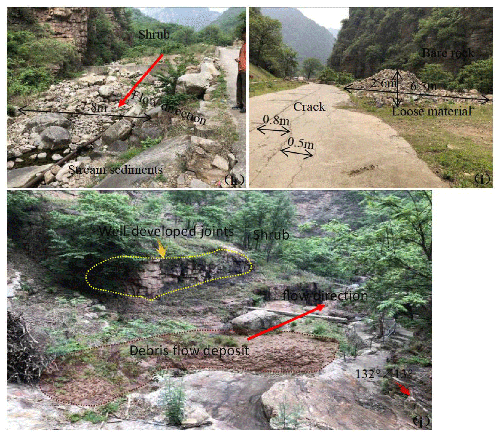
Figure 5Lishu scenic spot. h is stream sediments, i is road cracks and g is debris flow deposit.
3.1 Fuzzy C-means clustering (FCM)
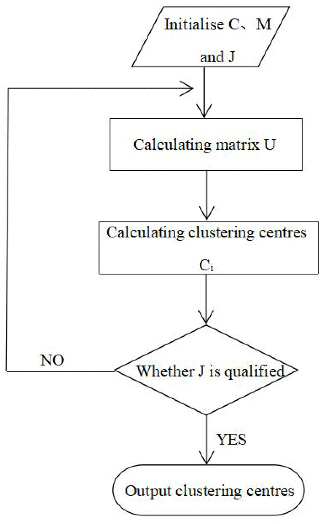
The fuzzy C-means method belongs to soft clustering, which is widely used at present. Its core idea is to map data points of a multi-dimensional space to different clustering sets in the form of membership degree so as to determine C cluster centres in such a manner that the intercluster associations are minimised and the intracluster associations are maximised (Bezdek, 1981). For every group, each point is assigned a membership degree between 0 and 1. The membership values indicate the probability of each point belonging to the different groups (Eke et al., 2019). The steps of the FCM algorithm are as follows (Fig. 6).
-
The membership matrix μij is initialised with random numbers between 0 and 1, which are used to represent the membership degree of xi to the cluster j; it satisfies the constraint conditions
where C represents the number of clusters.
-
For calculating clustering centres Ci, the formula is as follows (Hammah and Curran, 1998):
where m controls the degree of fuzziness and m=2 is deemed to be the best for most applications (Bezdek, 1981). Xj represents the jth sample.
-
For determining the number of clustering centres, the clustering number C of the FCM algorithm is not clearly given, which is one of the key factors affecting the clustering effect. So this paper combines the non-distance-based FCM clustering effectiveness index proposed by Chen and Pi (2013) to determine the value of C. The exponent (Vcs) consists of the compactness index and separation index. The definition of compactness is as follows:
where Cij is the compactness of the jth sample with the ith. When uij is greater than or equal to 1∕c, it avoids being meaningless for being too small. When , this indicates that the J sample is unlikely to belong to the ith class. When all samples clearly belong to a certain class, the compactness degree is the maximum – that is, the clustering result is compact. We define the whole compactness of sample data as follows:
The definition of the separation index is as follows:
namely, the minimum value of the membership degree of samples belonging to these two categories. When the division of the two categories is relatively clear, this indicates that the membership degree of samples belonging to a certain category must be greater than other values. Therefore, the better the clustering result is, the smaller Sij should be, and the total separation is defined as
The smaller the dispersion is, the greater the difference between the two classes is and the better the clustering result is.
Based on this, the clustering effectiveness Vcs index is defined as follows:
In conclusion, when C is larger and the S value is smaller, Vcs is larger and the clustering effect is better.
-
Calculating the value function J,
where N is the total number of observations, and j is the fuzzy objective function; d2 is the Euclidean distance between the ith clustering centre and the jth data point (Wang et al., 2008).
The operation is stopped when J is less than a certain threshold.
-
Calculating the new matrix Uij and returning to step 2,
3.2 Factor analysis
FA is a multivariate statistical analysis method which studies the internal dependence of variables and reduces some variables with intricate relations to a few comprehensive factors (Li et al., 2016). FA is the inferred decomposition of observed data into two matrices. One matrix represents a set of underlying unobserved characteristics of the subject which give rise to the observed characteristics and the other explains the relationship between the unobserved and observed characteristics (Tolkoff et al., 2018). The mathematical formula can be expressed as follows:
where X(x1, x2, …, xp) is the original factor; F(F1, F2 …, Fm) is the common factor; A=(akj), p×m, is the factor-loading matrix; akj represents the load of the k original factor on the J common factor; and ε=(ε1, ε2, …, εp) is a special factor.
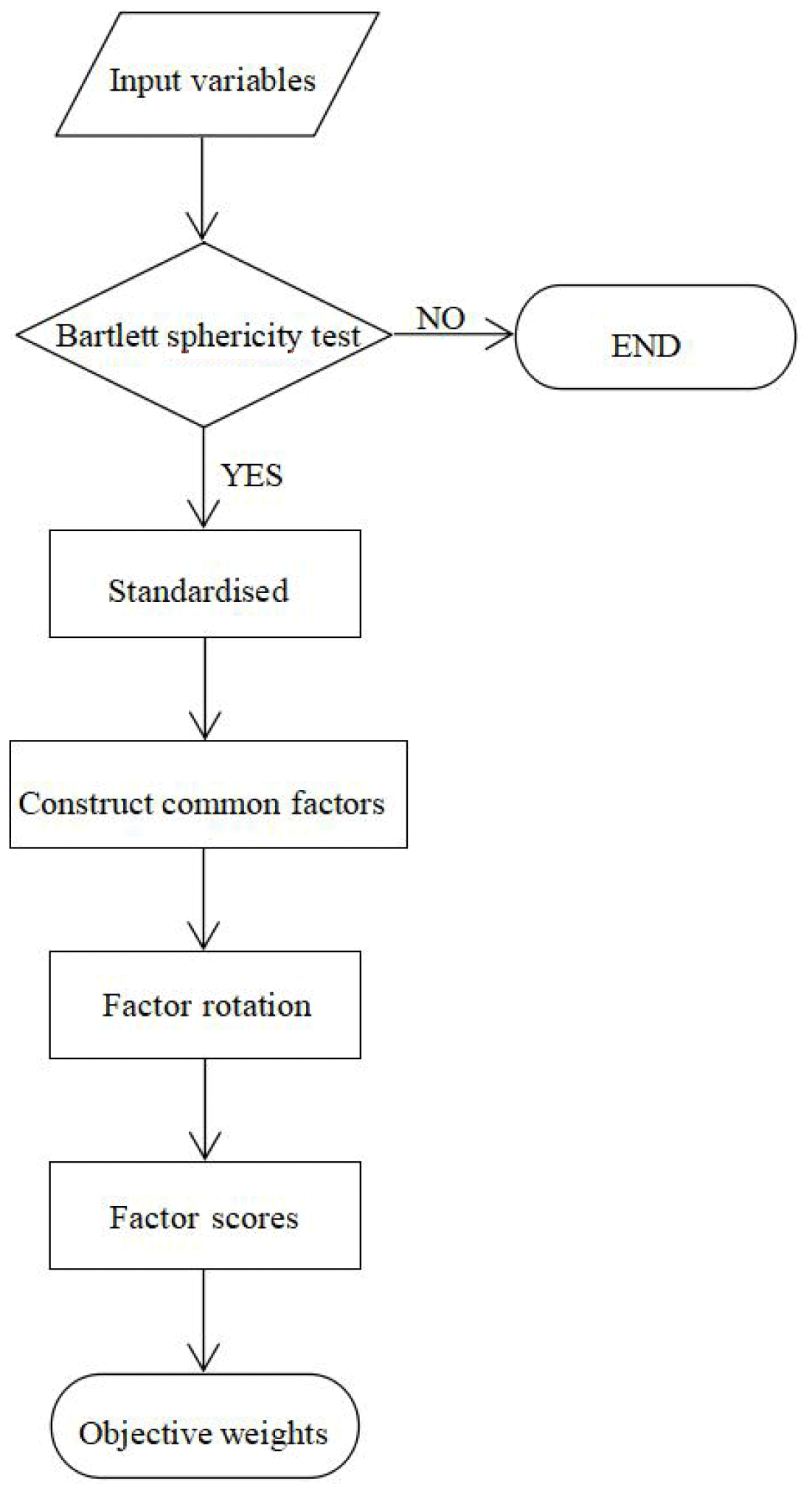
The main calculation steps of the factor analysis method can be divided into six steps (Fig. 7).
-
Test the feasibility of FA of original evaluation index variables. In this paper, SPSS was used to provide a Bartlett sphericity test to determine whether variables are suitable for FA.
-
Standardised calculation of original data. In order to eliminate the numerical differences of different variables in the order of magnitude and dimension, the original data should be standardised. This paper adopted the Z standardisation method in SPSS software.
-
Construct a common factor F. In the study, the first m factors for which the cumulative variance contribution rate is no less than 85 % were selected as common factors to represent the original data.
-
Factor rotation. In this paper, varimax orthogonal rotation was used to realise factor rotation.
-
Calculating factor scores. The most common method for calculating factor scores is the Thomson regression method (Tolkoff et al., 2018), and the formula is as follows:
where is factor-scoring coefficient matrix and A is the factor-loading matrix after rotation.
-
Calculating weight. The product of the factor-scoring coefficient and variance contribution rate is the contribution of each factor in the sample, and the sum of the contribution of each factor divided by the contribution of all indices is the weight of each factor. It is expressed by the formula
where βji is the coefficient score of each index in principal component Fj; i=1, 2, …, p; j=1, 2, …, m; and e is the contribution rate of factor variance.
3.3 Combination weighting method
Considering the defects of the current method for determining the weight of factors, the combination of a analytic hierarchy process and factor analysis method is used to determine the weight of each influencing factor of debris flow.

3.3.1 Analytic hierarchy process (AHP)
The AHP was first proposed by Saaty (1978), a famous American mathematician. It decomposes the factors related to decision-making into multiple layers, such as the target layer, criterion layer and scheme layer. The AHP is a subjective weighting method and has obvious advantages in determining the weight of each factor. The specific steps are as follows.
-
Establishing a hierarchical structure model. The hierarchical structure is mainly divided into three layers: the target layer, criterion layer and scheme layer.
-
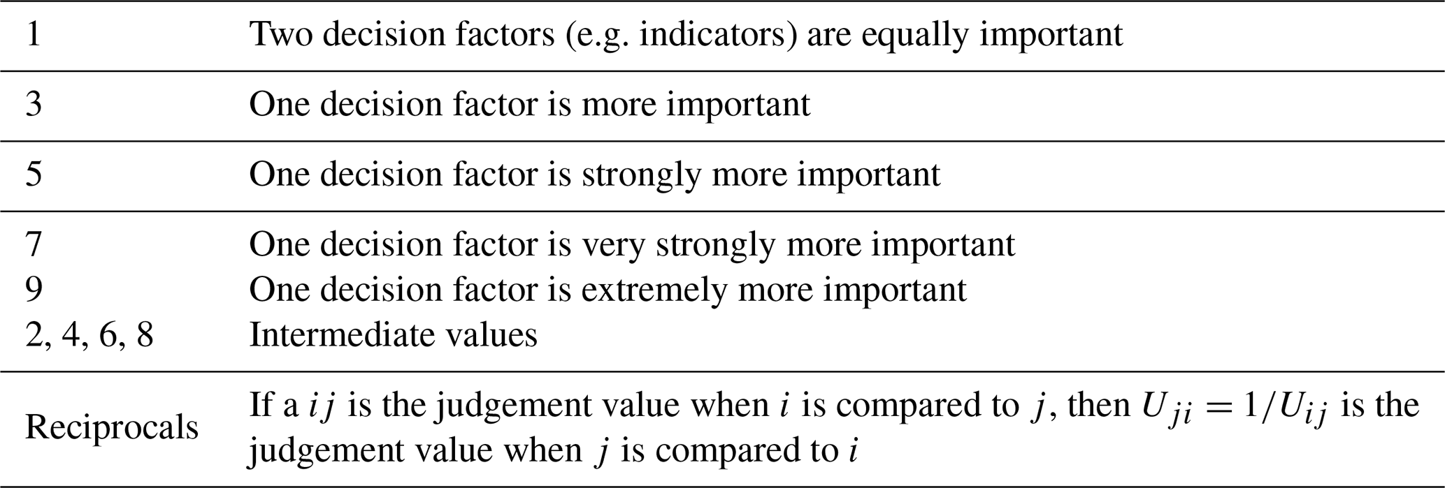
Establishing the judgement matrix. For the same level, the judgement matrix is established by pairwise comparison. The formula is as follows:
where aij is the ratio of relative importance between element Bi and Bj, which is usually expressed by the scoring method from 1 to 9 (Saaty, 1978), as shown in Table 2.
-
Consistency testing. The consistency test is divided into three steps. Calculating the consistency index (CI) (Saaty, 1977a, b), the expression is
where λmax is the largest eigenvalue of the judgement matrix A.
-
Average random consistency RI. RI is associated with the order of the judgement matrix, and their relationship is shown in Table 1.
-
Obtaining the test coefficient CR. This can be calculated by the following equation:
If CR < 0.1, the judgement matrix has a good consistency with reasonable judgement. Otherwise, the judgement matrix needs to be revised until the consistency test is satisfied.
Table 3Factors frequently used in susceptibility analysis of debris flow.
3.3.2 Combination weighting rule
The weight value obtained by the AHP is set as , and the weight value obtained by FA is set as (Feng et al., 2010), as shown in Eq. (16):
where α and β are weight coefficients calculated through the AHP and factor analysis method, respectively; rij is the standardised value of the jth influencing factor of the ith debris flow. α and β are determined according to the following formula:
The combined weight () can be represented by Eq. (18):
3.4 Efficiency coefficient method
Based on the principle of multi-objective programming, the efficiency coefficient method transforms each factor into a measurable evaluation score through the efficiency function and combines the weight of factors to make a comprehensive evaluation. The specific steps are as follows.
-
Select the evaluation factors.
-
Determine the satisfactory value and the unallowable value: the satisfactory value is a value based on years of experience, while the unallowable value is the lowest or highest acceptable value of the evaluation index.
-
Calculate the single efficacy coefficient. The single efficacy coefficient was calculated by the corresponding efficacy function based on the sensitivity of each factor. It is mainly divided into three variables: the extremely large variable (the higher the factor, the higher the efficiency coefficient), the infinitesimal variable (the smaller the index value, the larger the efficiency coefficient value) and the interval variable (the value reaches its highest in a certain interval). The specific formula is as follows:
where g1i is the single efficacy coefficient value of the ith extremely large factor, Xi is the actual value of the ith factor, Xyi is the satisfactory value of the ith factor and Xni is the unallowable value of the ith factor.
The infinitesimal variable is calculated as follows:
The interval variable is calculated as follows:
-
Calculating the total efficiency coefficient,
where G is the total efficacy coefficient, gi is the single efficacy coefficient and ωi is the weight of the ith factor.
The flowchart for the method used for our classification and susceptibility analysis is shown in Fig. 8.
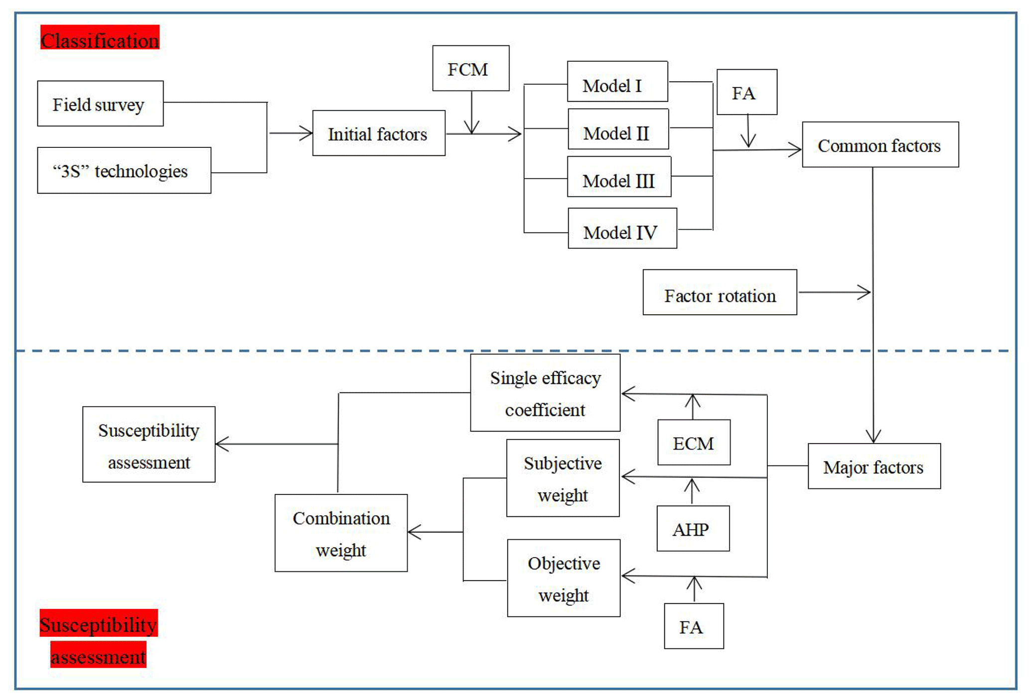
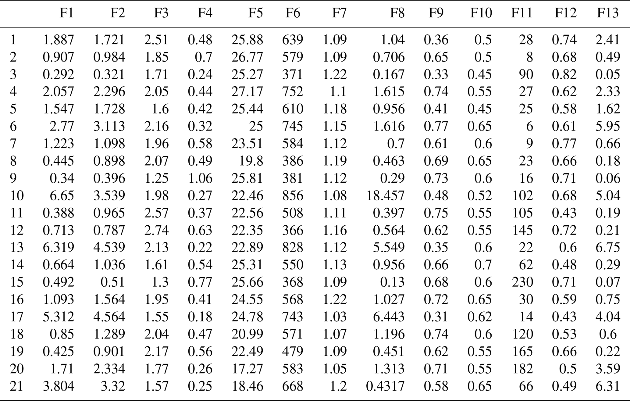
Table 4The values for the 13 factors of the 21 debris flow catchments.
3.5 Influencing factors
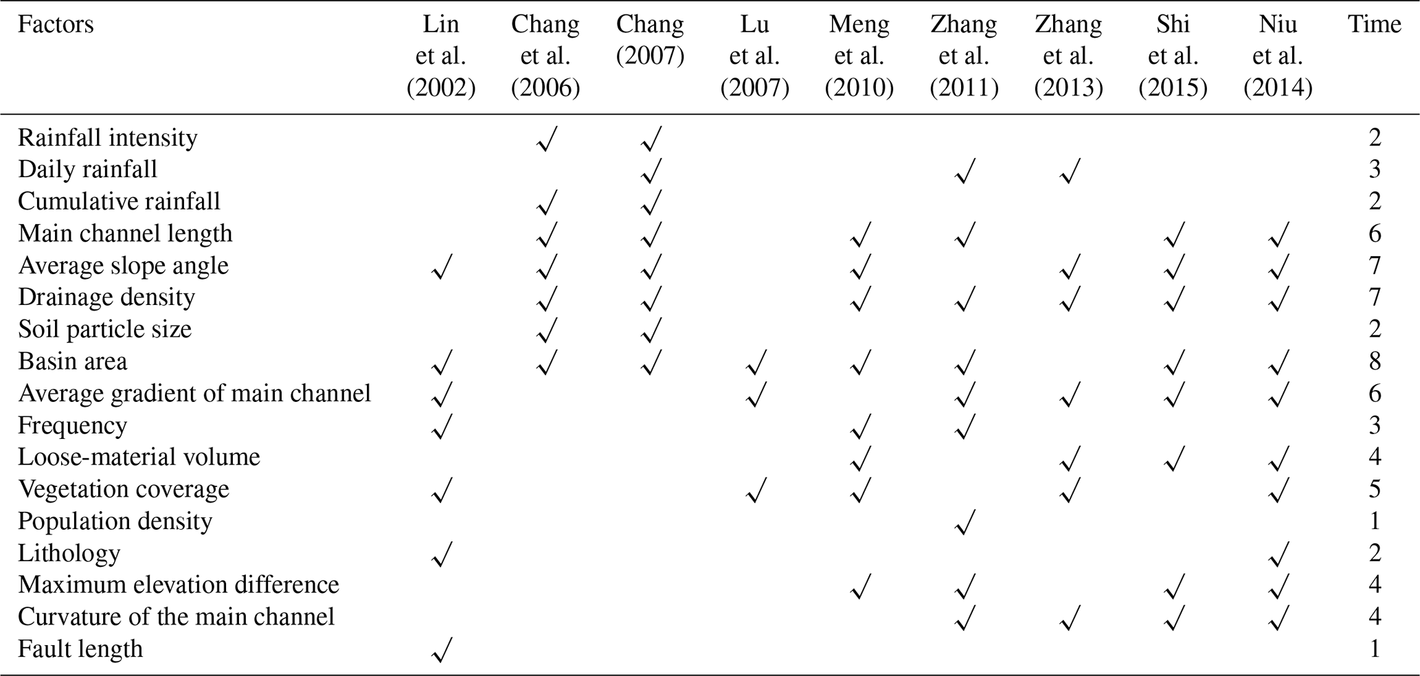
The topographical, geological and climatic factors play a critical role in the distribution and activities of debris flows (Di et al., 2008). Table 3 shows the influencing factors selected by research in debris flow susceptibility assessment in recent years. Rainfall is one of the most pivotal external factors inducing debris flow disasters, but the meteorological data in our area are all from the same station, which cannot reflect the differences between each catchment. Therefore, rainfall was not included in this study. In addition, the frequency of debris flow and the size of soil particles are difficult to obtain accurately. The loose-material volume reflects the lithological characteristics and fault length to some extent, so lithology and fault length were not taken into account. The basin area, main channel length, drainage density, average slope angle, average gradient of the main channel, vegetation coverage, maximum elevation difference and curvature of the main channel, which were cited and available, were selected in this paper. As source conditions, the loose-material volume and the loose-material supply length ratio were also considered. As the study area is located in a tourist area with a relatively dense population, population density is selected as the factor of human activities. A total of 13 influencing factors were selected based on the previous research findings to reflect the characteristics of the watershed. All these factors were acquired in our field survey or calculated in ArcGIS, as described below.
-
Basin area (F1) (km2). The basin area reflects the scale of debris flow. Generally, the larger the basin area is, the greater the risk of debris flow will be. It was obtained by geometric operations in ArcGIS and corrected by the remote-sensing images in Google Earth.
-
Main channel length (F2) (km). Main channel length reflects the potential for increasing loose sources along the route. This value was measured from ArcGIS by combining RS technology and topographic maps.
-
Drainage density (F3) (km km−2). Drainage density is the ratio of the total drainage length to the watershed area, and it is an important index for describing the development of gullies in the watershed.
-
Average gradient of the main channel (F4). This is the ratio of the maximum elevation difference of the main channel to its linear length. The larger the value, the better the hydrodynamic condition is. This value is obtained from the digital elevation model (DEM).
-
Average slope angle (F5) (∘). As F5 increases, the erosion capacity and intensity of precipitation increase. The value was obtained by the ArcGIS slope analysis tool.
-
Maximum elevation difference (F6) (m). The difference between the maximum and minimum elevation values in the basin provides the kinetic energy condition of disaster. This value is also obtained from the DEM.
-
Curvature of the main channel (F7). F7 is the ratio of the main channel length to its linear length, which reflects the degree of channel blockage.
-
The loose-material volume (F8) (×104 m3). The loose material is one of fundamental factors triggering debris flows. This factor is obtained through field investigation with tape and a laser rangefinder. The thickness was obtained by field estimation and a trench test.
-
The loose-material supply length ratio (F9). F9 is the ratio of loose-material length along a channel to total channel length, which reflects the successive supplied sediments. It was obtained through field surveys and RS technology.
-
Vegetation coverage (F10). The lower the vegetation coverage, the more serious the soil erosion. It was estimated from field surveys and SPOT5 imaging.
-
Population density (F11) (number of people per km2). With the development of social economy, human activities have gradually become an important factor affecting debris flow. Population density reflects the intensity of human activities, which is estimated according to the number of buildings through field survey and RS technology.
-
Roundness (F12). Roundness is the morphological statistical element of a gully, and the plane shape of a gully differs from its developmental stage. F12 is the ratio of the length of the main channel of debris flow to its area.
-
The highest volume of one flow (F13) (×104 m3). Liu et al. (1993) selected F13 as the main factor in the risk assessment of debris flow, which is one of the most important factors in evaluating the degree of debris flow hazard.
4.1 Fuzzy C-means clustering analysis
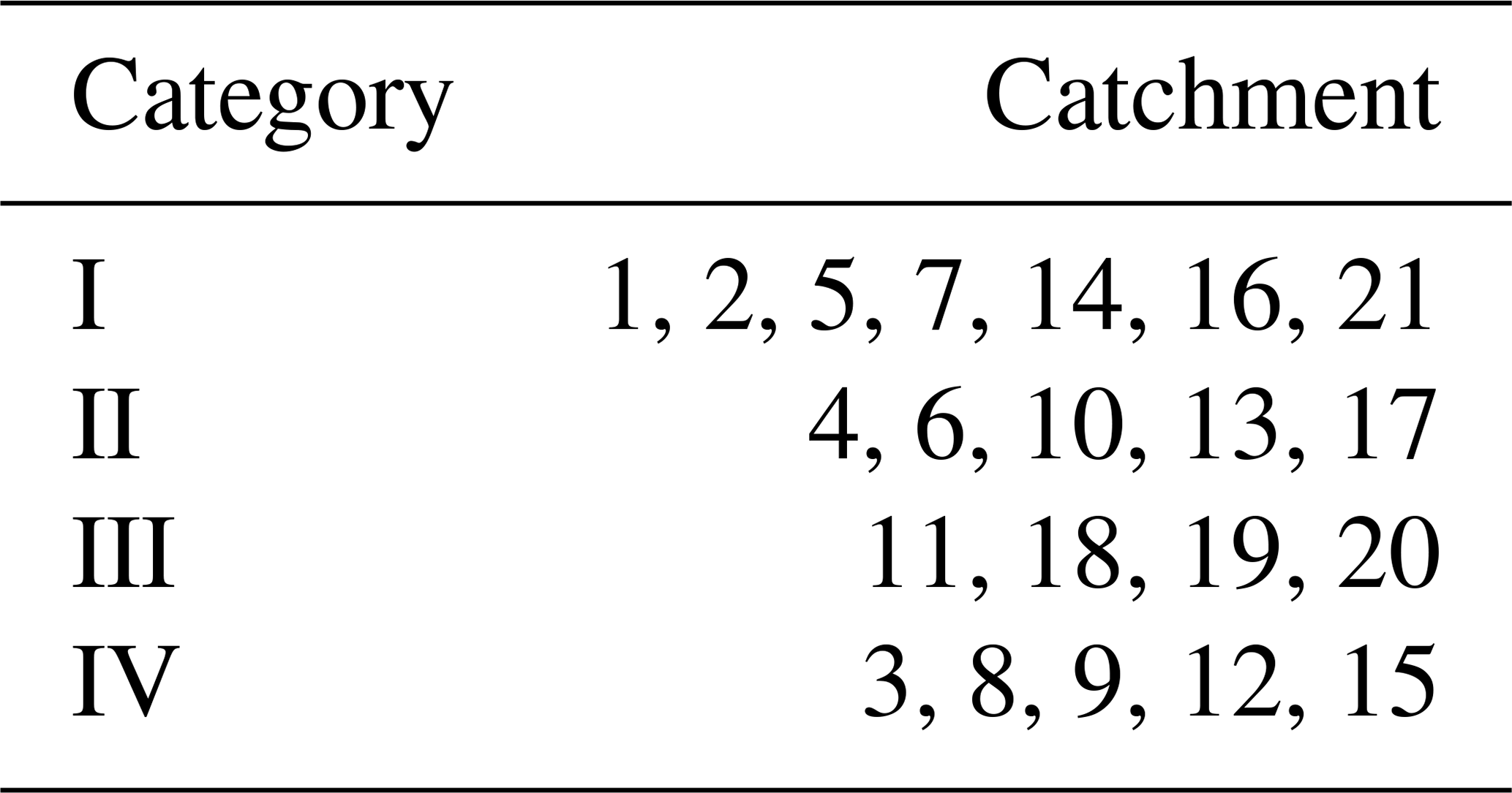
The curve of the clustering effectiveness index Vcs with the number of clustering centres is shown in Fig. 9, and the optimal number of clustering centres is four. Based on the basic data of 21 debris flow catchments, the FCM was carried out and set the fuzzy weighted index to m=2. The results are shown in Table 5.

Thus 21 debris flow catchments in the study area are divided into four categories. The data of each catchment belonging to the same category have a certain internal similarity and vary greatly among different categories. In other words, data of different influencing factors have different effects on different types of debris flows, which provide a favourable basis for us to analyse the main influencing factors of debris flows, and also point out the direction for monitoring and prevention of debris flows.
4.2 Factor analysis
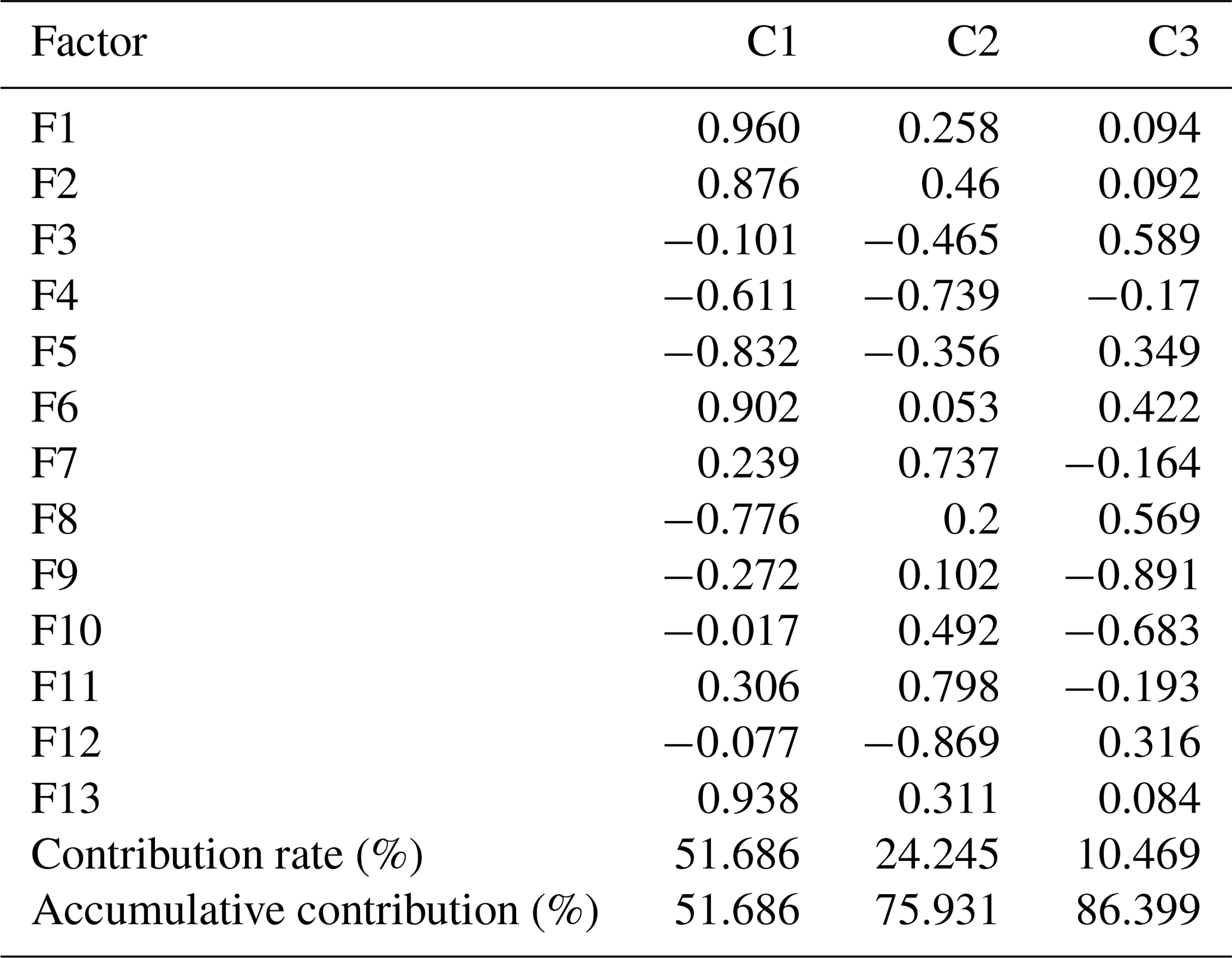
Based on the clustering results of 21 debris flow catchments, FA was used to analyse each type of debris flow. Tables 6–9 are the results of the first, second, third and fourth categories, respectively.
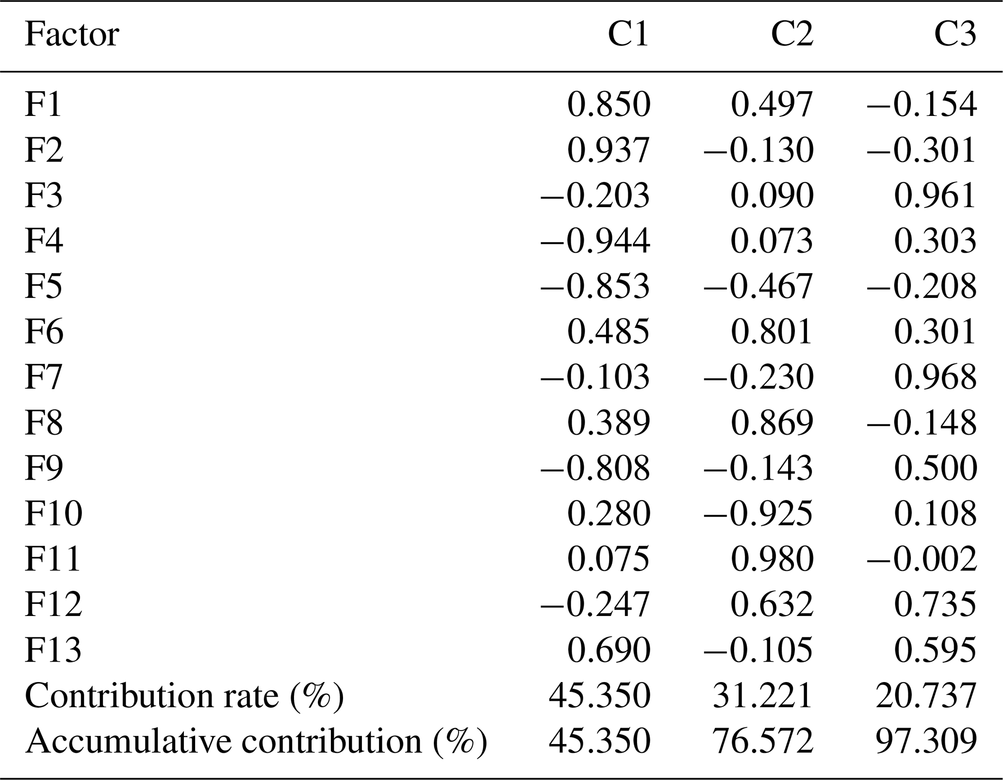
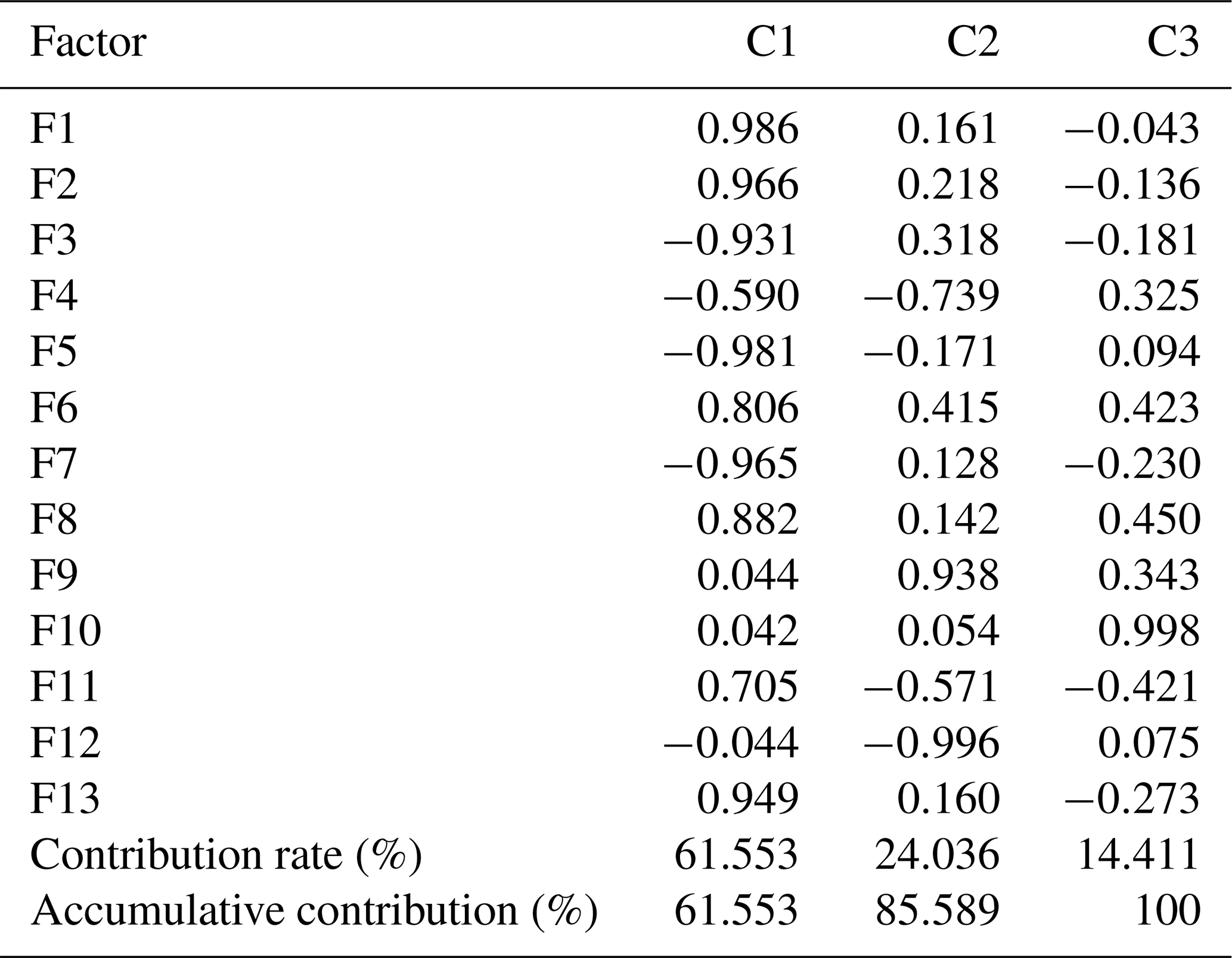
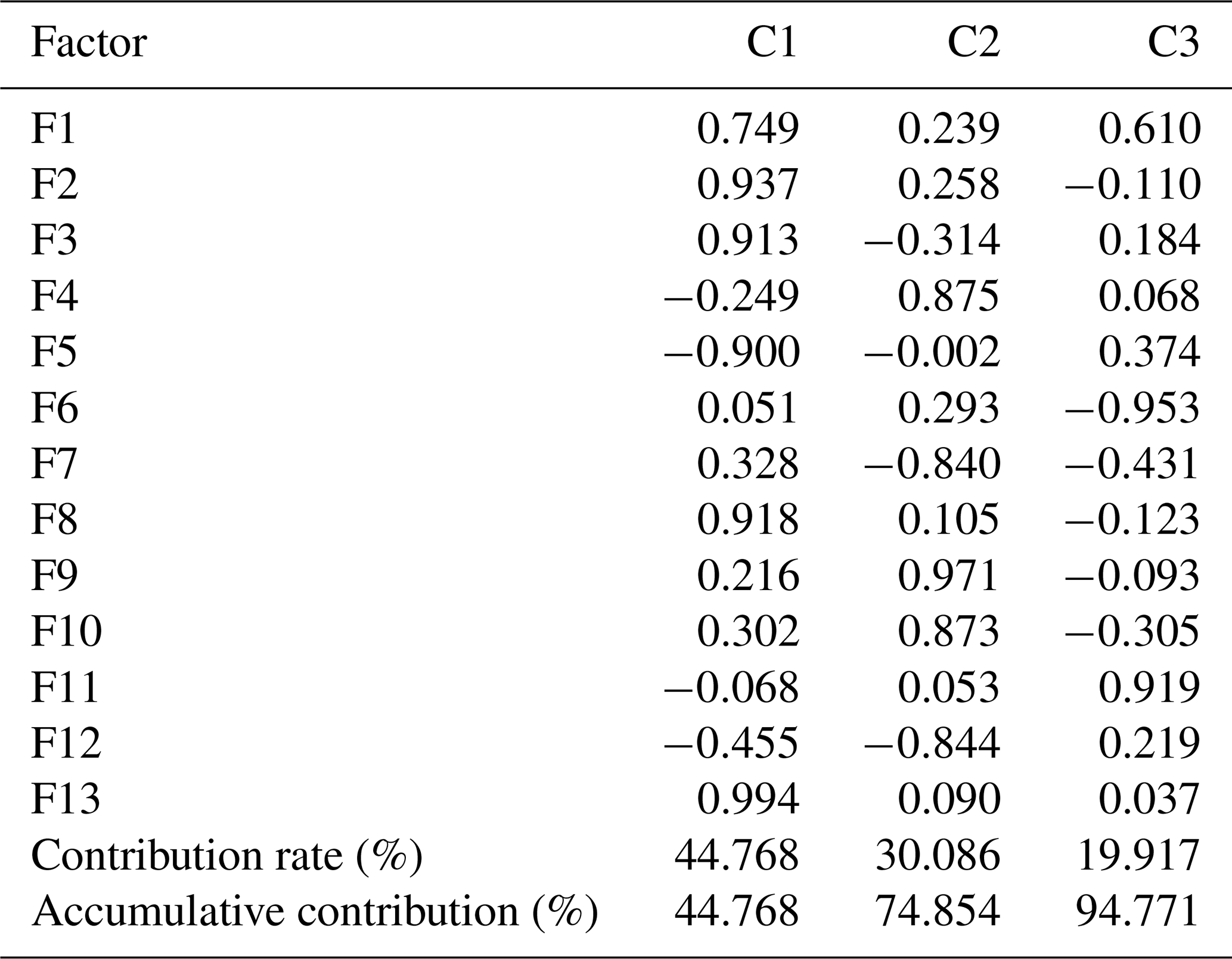
As shown in Table 2, in the first category, the accumulative contribution rate of the first three factors (C1–C3) reaches 86.40 %, which retains most information of the 13 original variables. For the first group, the load values of the main factors 1–3 are relatively large in the basin area, the highest volume of one flow, the maximum elevation difference, the main channel length and curvature of the main channel, and population density and drainage density. Similarly, in the second type, the load values of the main factors 1–3 are relatively large in the basin area, the main channel length and population density, loose-material volume and drainage density, and maximum elevation difference. In the third category, the load values of the main factors 1–3 are relatively large in the basin area, main channel length, the highest volume of one flow, loose-material volume, and the loose-material supply length ratio and vegetation coverage. In the fourth category, the load values of the main factors 1–3 are relatively large in main channel length, drainage density, loose-material volume, the highest volume of one flow, and the loose-material supply length ratio and population density.
Table 6The factor-loading matrix after rotation and contribution ratios for the first category.
Among the 13 factors, the basin area and the highest volume of one flow reflect the scale of debris flow eruption. The main channel length, drainage density, average gradient of the main channel, the average slope, maximum elevation difference, curvature of the main channel and roundness reflect the topographical condition. The loose-material volume and the loose-material supply length ratio are the material sources for debris flow. Vegetation coverage reflects the geomorphologic condition. Population density reflects the impact of human activities on nature to some extent. Therefore, four types of debris flows can be named according to the results of the FCM and FA.
Table 7The factor-loading matrix after rotation and contribution ratios for the second category.
The first category can be defined as debris flow closely related to scale–topography–human activities. Considering the situation, monitoring and control of basic material sources is recommended. Similarly, the second, third and fourth categories can be defined as topography–human activities–provenance, scale–provenance–topography and topography–scale–provenance–human activities, respectively. In the same way, corresponding prevention measures can be proposed according to the characteristics of each type of debris flow.
Table 8The factor-loading matrix after rotation and contribution ratios for the third category.
4.3 Weights of major factors
Based on the FA of each category of debris flow in the previous section, the main influencing factors were obtained. However, the repeatability of evaluation information should be reduced. Average slope angle and average gradient of the main channel are both indicators of potential energy, so the average gradient of the main channel is omitted. Similarly, curvature of the main channel, the loose-material supply length ratio and roundness were omitted. Thus nine factors, including basin area (F1), main channel length (F2), drainage density (F3), average slope angle (F5), maximum elevation difference (F6), the loose-material volume (F8), vegetation coverage (F10), population density (F11) and the highest volume of one flow (F13) were selected. On the other hand, a reduction in the number of indicators facilitates the allocation of weight values.
Table 9The factor-loading matrix after rotation and contribution ratios for the fourth category.

4.3.1 Subjective weights
The AHP was applied to calculate the subjective weight in this paper. The hierarchical structure (Fig. 10) was constructed, and the 1–9 scale method was used to grade each factor. The judgement matrices (Table 10) and (Table 11) were constructed, and the consistency test was conducted. The weight values of each factor are shown in Table 12.
Table 10Comparison matrix elements for geology condition.
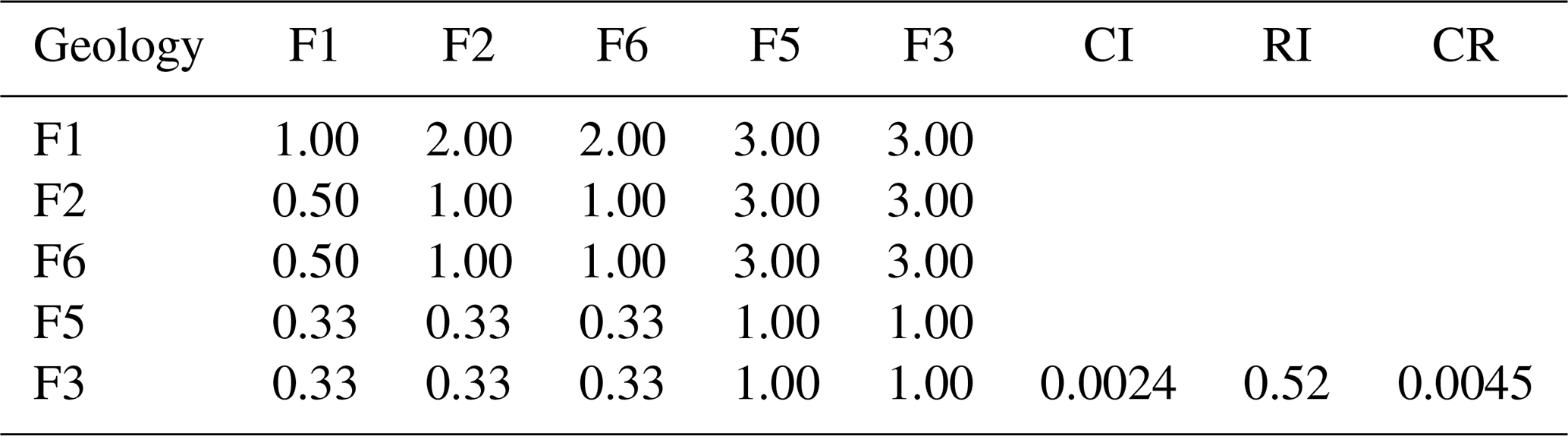
CR = 0.0045<0.1 met the conformance inspection requirements.
Table 11Comparison matrix elements of the criterion level factors.
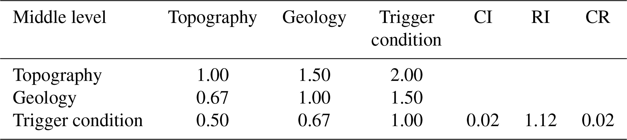
CR = 0.02<0.1 met the conformance inspection requirements.
4.3.2 Objective weights
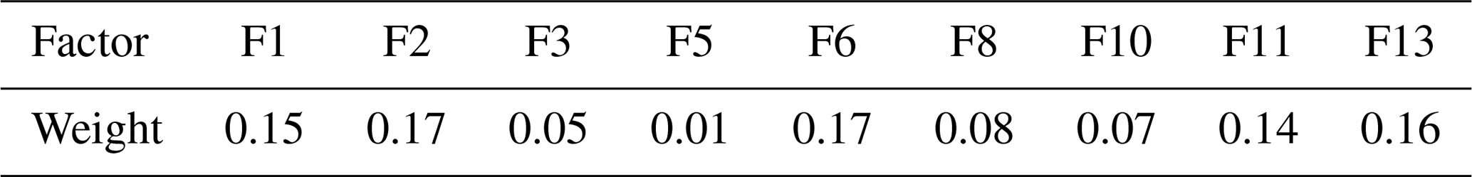
FA was applied to calculate the objective weight in this paper. The weight values of each factor are shown in Table 13.

Table 13The weighted values of the factors obtained by factor analysis.
4.3.3 Combination weights
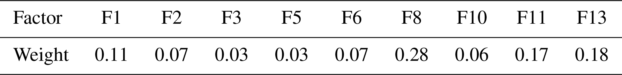
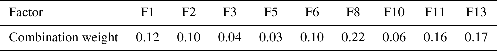
After the subjective weight and objective weight are obtained, the respective distribution coefficients are solved according to Eq. (1), and the final combined weight values of each factor are shown in Table 14: α=0.70, β=0.30; F8 > F13 > F11 > F1 F2 = F6 > F10 > F3 > F5.
4.4 The efficacy coefficient of factors
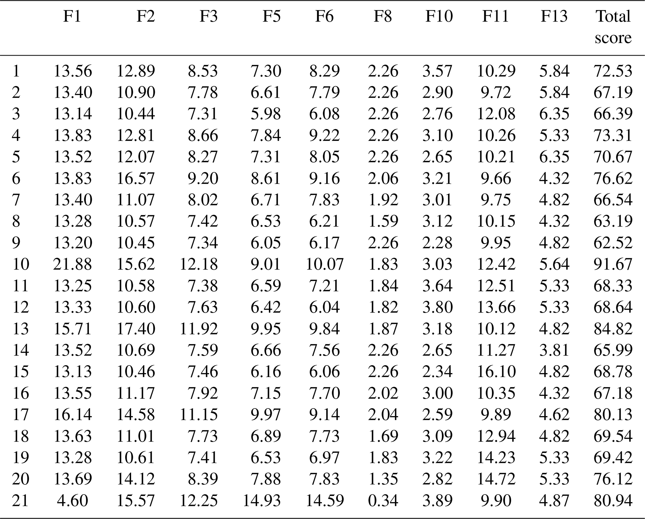
Among the nine factors, basin area, main channel length, drainage density, maximum elevation difference, the loose-material volume, the highest volume of one flow and population density are all extremely large variables. Vegetation coverage is the infinitesimal variable. The average slope angle is an interval variable. Table 15 shows the efficacy coefficient scores of 21 debris flow catchments after being combined with the weight calculation.
Table 15The efficacy coefficient scores of 21 debris flow catchments.
4.5 Susceptibility assessment of debris flow
Taking the total efficiency coefficient of each catchment as the evaluation standard (the larger the value, the higher the possibility of debris flow), the FCM was conducted for 21 debris flow catchments in the study area. The result showed that the susceptibility of debris flow was divided into three grades: high (H), moderate (m) and low (L). Combined with the classification of each debris flow mentioned above, the final results are shown in Table 16.
Table 16The qualitative description and susceptibility class for each debris flow catchment.
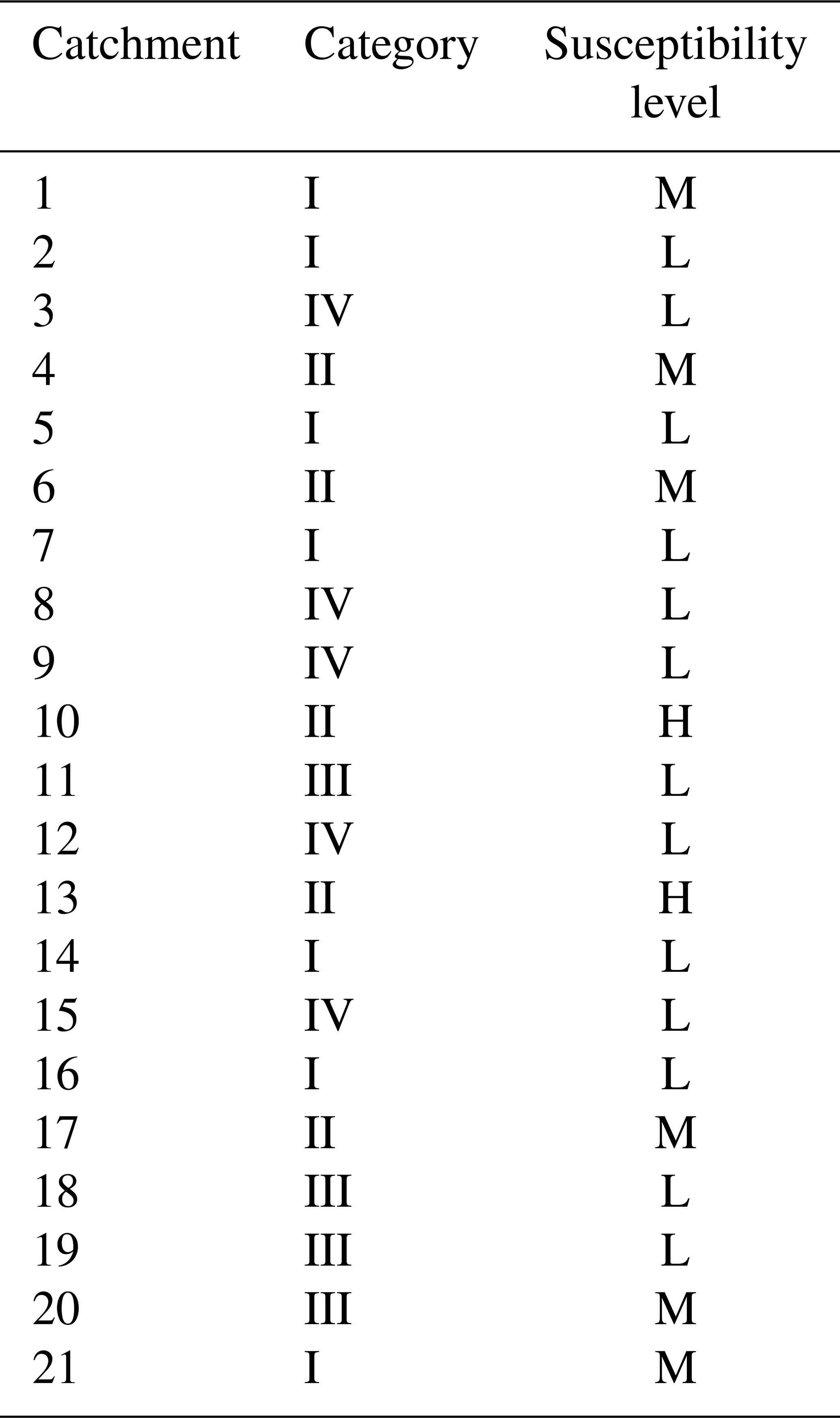
As shown in Table 16, susceptibility for the 10th and 13th catchments was high, and both of them belong to the debris flow with a close relationship between topography, human activities and provenance. Susceptibility for six catchments, including the 1st, 4th, 6th, 17th, 20th and 21st, was medium. The other 13 had low susceptibility.
Normative scoring, the k-means clustering algorithm and hierarchical clustering were determined to validate susceptibility analysis methods used in this paper.
Based on the field investigation, the 10th catchment is located in Huangsongyu National Mining Park, where a large amount of slag accumulated. With low vegetation coverage and steep terrain, the gully was in its prime, which directly threatened the safety of villagers and tourists. What is more, there are several warning boards for natural disasters and corresponding monitoring equipment in the scenic spot (as shown in Fig. 5). The 13th catchment is located in the Lishugou village scenic spot. Part of the pedestrian passageway was built, but a lot of stones were piled up in the trench and the road was broken and steep (as shown in Fig. 6). However, there is no obvious accumulation of loose materials in the catchments with low susceptibility. The gully was in its old stage, with high vegetation coverage and little human interference. The quantitative comprehensive evaluation results of debris flow susceptibility are shown in Table 17, which are divided into two levels: low (L) and moderate (M). Among them, the susceptibility levels of the 10th and the 13th catchments were moderate and the others were low.
Table 17Comparison of susceptibility analyses based on different algorithms.
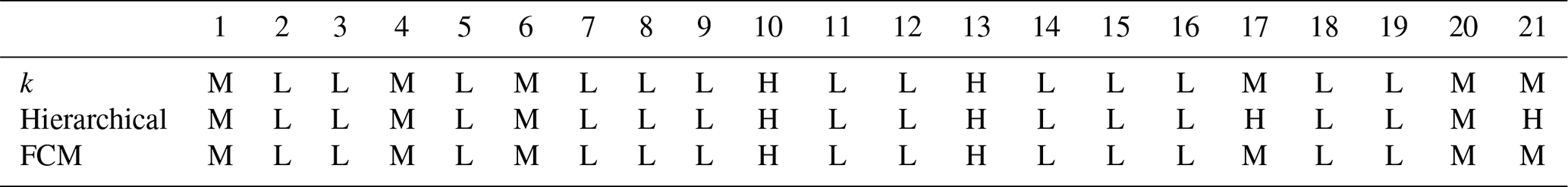
The k-means clustering algorithm (k) (Hartigan and Wong, 1978) and hierarchical clustering (H) (Kimes et al., 2017) were used for the classification of our data to measure the classification performance in this paper. The results are shown in Table 17. The susceptibility results obtained by k and the FCM are exactly the same. The susceptibility assessment of 17th and 21st were high when based on H and moderate from the FCM and k. However, such minor differences are acceptable. On the other hand, the susceptibility results obtained by the FCM and normative scoring are different. This is mainly because the number of categories is different, and the level was generally higher when obtained by the FCM. In addition, it can be seen from the tree graph (Fig. 11) obtained by hierarchical clustering that the clustering results are more reasonable when divided into three categories, which is consistent with Vcs. Therefore, the susceptibility model established in this paper is suitable and reasonable.
The accuracy of the debris flow classification directly affects the development of prevention and control measures. Based on different criteria, such as genetic classification, occurrence frequency and material composition, the same debris flow can belong to multiple categories at the same time, which does not reasonably reflect its multiple characteristics. In addition, the traditional classification standard has some hysteresis to prevent debris flow. Considering that different types of debris flow have different main influencing factors, the FCM and FA were combined in this study to refine and summarise the importance of various factors to improve the accuracy of the classification. The FCM is different from traditional rigid division, and it is based on the distance function to calculate the maximum correlation between the same kind of data and the minimum correlation between different kinds of data (Eke et al., 2019). The clustering effectiveness Vcs was introduced to effectively solve the problem of determining the number of clusters, and the clustering analysis was carried out on the basic data of 21 debris flow catchments. FA is a primary exploratory tool for dimension reduction and visualisation (Verde and Irpino, 2018). The main influencing factors of each category are obtained by FA, which not only realises effective dimensionality reduction but also eliminates the linear relationship between factors. The results showed that different kinds of debris flows obtained by the FCM had different major influencing factors. In other words, data for different influencing factors have different effects on different types of debris flows, which demonstrates the advantages of the FCM when combined with the factor analysis. According to different main influencing factors, the development characteristics of debris flows can be reclassified. This also provided an effective basis for us to study the origin and classification of debris flow and point out the direction for monitoring and controlling disasters.
The reasonable selection of evaluation factors is the premise of accurate evaluation of debris flow susceptibility. In this paper, 13 factors were preliminarily selected based on previous experience and field investigation conditions. Secondary screening was carried out based on FA analysis results, which enhanced the rationality of the screening. The determination of the factor weight is crucial to accurately evaluating the susceptibility of the debris flow (Zhang et al., 2013). FA is a common objective evaluation method in statistical analysis that determines the weight of factors according to the internal correlation and patterns of data. However, the objective method cannot reflect the relative significance of each influencing factor and may create misleading information. The AHP can make full use of expert experience and achievements in the corresponding fields to evaluate the influencing factors, which is a subjective method. However, different researchers have different preferences for major factors, which have a negative impact on the results. Therefore, combination weighting, which combines the advantages of the FA and AHP, is superior to the other methods alone when trying to obtain a more scientific and reasonable evaluation result.
The efficiency coefficient method is different from other evaluation systems. By determining the satisfactory value of each factor as the upper limit and the unallowable value as the lower limit, the satisfaction degree is calculated through the corresponding efficiency function, and the final comprehensive score was obtained based on the weight evaluation. This method not only considers the relative importance of different factors but also determines the value based on the susceptibility to debris flow. Therefore, the efficiency coefficient method can objectively evaluate complicated research objects, such as debris flow, with this form of classification that conforms to logical thinking. However, the evaluation method adopted in this paper also has limitations: (1) fuzzy C-means clustering is not applicable to the evaluation of a single debris flow gully; (2) the factor analysis method is not applicable when the sample data are too small; (3) the tools used in field investigation are too simple, and some data, such as the loose-material supply length ratio, are not accurate enough; and (4) rainfall variations were not considered between different debris flows.
Classification and susceptibility analysis are of great significance for the early warning and prevention of debris flow. Based on field investigation and 3S technology, an improved FCM and FA method were used to establish the classification model and obtain the main influencing factors of different types of debris flow in the current study. The ECM was used for the susceptibility analysis based on the combination weights of major factors.
In this paper, 21 debris flow catchments in Beijing were divided into four categories. Nine major factors screened from the classification results were determined for susceptibility analysis using both the ECM and combination weighting, and the susceptibility assessment was divided into three levels, which have been validated with normative scoring, the k-means clustering algorithm and hierarchical clustering. An effective scientific classification and susceptibility assessment results of debris flow were obtained, which provides a theoretical basis for formulating disaster prevention and reduction plans and measures for debris flow. Therefore, a semi-quantitative evaluation method which combines fuzzy mathematics, multivariate statistical analysis and the geological environment is suitable for risk assessment for a study area with a limited number of samples. Different methods have their own advantages and disadvantages, and some methods are complementary to a certain extent, so it is desirable to enhance the rationality of the application through the combination of multiple methods.
The data used to support the findings of this study are included within the article.
ZL was responsible for the writing and graphic production of the paper. CW was responsible for the revision of the paper. SH was responsible for part of the calculations. KUJK was responsible for the translation. YL was responsible for the reference proofreading.
The authors declare that they have no conflict of interest.
This article is part of the special issue “Resilience to risks in built environments”. It is not associated with a conference.
This work was supported by the National Natural Science Foundation of China (grant nos. 4197020250 and 41572257).
This research has been supported by the National Natural Science Foundation of China (grant nos. 41572257 and 4197020250).
This paper was edited by Mattia Leone and reviewed by Daniele Masi and one anonymous referee.
Aguilar, O. and West, M.: Bayesian dynamic factor models and portfolio allocation, J. Bus. Econ. Stat., 18, 338–357, 2000.
Benda, L. E. and Cundy, T. W.: Predicting deposition of debris flows in mountain channels, Can. Geotech. J., 27, 409–417, 1990.
Bezdek, J. C.: Pattern recognition with fuzzy objective function algorithms, in: IEEE Electrical Insulation Magazine, Plenum Press, New York, 1981.
Blais-Stevens, A. and Behnia, P.: Debris flow susceptibility mapping using a qualitative heuristic method and Flow-R along the Yukon Alaska Highway Corridor, Canada, Nat. Hazards Earth Syst. Sci., 16, 449–462, https://doi.org/10.5194/nhess-16-449-2016, 2016.
Brayshaw, D. and Hassan, M. A.: Debris flow initiation and sediment recharge in gullies, Geomorphology, 109, 122–131, 2009.
Burton, A. and Bathurst, J. C.: Physically based modelling of shallow landslide sediment yield at a catchment scale, Environ. Geol., 35, 89–99, 1998.
Carrara, A., Crosta, G., and Frattini, P.: Comparing models of debris-flow susceptibility in the alpine environment, Geomorphology, 94, 353–378, 2008.
Chang, T. C.: Risk degree of debris flow applying neural networks, Nat. Hazards, 42, 209–224, 2007.
Chang, T. C. and Chao, R. J.: Application of back-propagation networks in debris flow prediction, Eng. Geol., 85, 270–280, 2006.
Chen, J. and Pi, D.: A Cluster Validity Index for Fuzzy Clustering Based on Non-distance, in: Proc. of the 5th International Conference on Computational and Information Sciences, 2013 China, 880–883, 2013.
Chiou, I.-J., Chen, C.-H., Liu, W.-L., Huang, S.-M., and Chang, Y.-M.: Methodology of disaster risk assessment for debris flows in a river basin, Stoch. Environ. Res. Risk Assess., 29, 775–792, 2015.
Clague, J. J., Evans, S. G., and Blown, J. G.: A debris flow triggered by the breaching of a moraine-dammed lake, Klattasine Creek, British Columbia Canadian, J. Earth Sci., 22, 1492–1502, 1985.
Conway, S. J., Decaulne, A., Balme, M. R., Murray, J. B., and Towner, M. C.: A new approach to estimating hazard posed by debris flows in the West fjords of Iceland, Geomorphology, 114, 556–572, 2010.
Di, A. F., Chen, N. S., Cui, P., Li., Z. L., He, Y. P., and Gao, Y. C.: GIS-based risk analysis of debris flow: an application in Sichuan, southwest China, Int. J. Sediment Res., 2, 138–148, 2008.
Eke, S., Clerc, G., Aka-Ngnui, T., and Fofana, I.: Transformer condition assessment using fuzzy C-means clustering techniques, IEEE Elect. Insul. Mag., 35, 47–55, 2019.
Feng, Q. G., Zhou, C. B., Fu, Z. F., and Zhang, G. C.: Grey fuzzy variable decision-making model of supporting schemes for foundation pit, Rock Soil Mech., 30, 2226–2231, 2010.
Glade, T.: Linking debris-flow hazard assessments with geomorphology, Geomorphology, 66, 189–213, 2005.
Gómez, H. and Kavzoglu, T.: Assessment of shallow landslide susceptibility using artificial neural networks in Jabonosa River Basin, Venezuela, Eng. Geol., 78, 11–27, https://doi.org/10.1016/j.enggeo.2004.10.004(1), 2004.
Hammah, R. E. and Curran, J. H.: Fuzzy cluster algorithm for the automatic identification of joint sets, Int. J. Rock Mech. Min. Sci., 35, 889–905, 1998
Hartigan, J. A. and Wong, M. A.: A K-means clustering algorithm, Appl. Stat., 28 100–108, 1978.
Iverson, R. M., Reid, M. E., and Lahusen, R. G.: Debris-flow mobilization from landslides, Annu. Rev. Earth Planet. Sci., 25, 85–138, 1997.
Kang, Z. C., Li, Z. F., and Ma, A. N.: Debris Flows in China, Science Press, Beijing, 2004.
Kimes, P. K., Liu, Y., Neil Hayes, D., and Marron, J. S.: Statistical significance for clustering, Biometrics, 73, 811–821, 2017.
Kritikos, T. and Davies, T.: Assessment of rainfall-generated shallow landslide/debris-flow susceptibility and runout using a GIS-based approach: application to western Southern Alpsof New Zealand, Landslides, 12, 1051–1075, 2015.
Li, X.-F., Chen, P., Han, W., Shi, H., and Yu, H.: Application of factor analysis to debris flow risk assessment, Chin. J. Geol. Hazard Contr., 27, 55–61, 2016.
Lin, P. S., Lin, J. Y., Hung, J. C., and Yang, M. D.: Assessing debris-flow hazard in a watershed in Taiwan, Eng. Geol., 66, 295–313, 2002.
Liu, X.-L., Tang, C., and Zhang, S.-L.: Quantitative judgment on the debris flow risk degree, J. Catastrophol., 8, 1–7, 1993.
Lu, G. Y., Chiu, L. S., and Wong, D. W.: Vulnerability assessment of rainfall-induced debris flows in Taiwan, Nat. Hazards, 43, 223–244, 2007.
Meng, F., Li, G., Li, M., Ma, J., and Wang, Q.: Application of stepwise discriminant analysis to screening evaluation factors of debris flow, Rock Soil Mech., 31, 2925–2929, 2010.
Mhaske, S. Y. and Choudhury, D.: GIS-based soil liquefaction susceptibility map of Mumbai city for earthquake events, J. Appl. Geophys., 70, 216–225, 2010.
Ni, H. Y., Zheng, W. M., Li, Z. L., Ba, R. J.: Recent catastrophic debris flows in Luding county, SW China: geological hazards, rainfall analysis and dynamic characteristics, Nat. Hazards, 55, 523–542, 2016.
Niu, C. C., Wang, Q., Chen, J. P., Wang, K., Zhang, W., and Zhou, F. J.: Debris-flow hazard assessment based on stepwise discriminant analysis and extension theory, Q. J. Eng. Geol. Hydrogeol., 47, 211–222, https://doi.org/10.1144/qjegh2013-038, 2014.
Peggy, A., McCuen, R. H., and Hromadka, T. V.: Magnitude and frequency of debris flows, J. Hydrol., 123, 69–82, https://doi.org/10.1016/0022-1694(91)90069-T, 1991.
Rickenmann, D.: Empirical Relationships for Debris Flows, Nat. Hazards, 19, 47–77, https://doi.org/10.1023/A:1008064220727, 1999.
Saaty, T. L.: A scaling method for priorities in hierarchical structures, J. Math. Psychol., 15, 234–281, 1977a.
Saaty, T. L.: Applications of analytical hierarchies, Math. Comput. Simul., 21, 1–20, 1977b.
Saaty, T. L.: Modeling unstructured decision problems – The theory of analytical hierarchies, Math. Comput. Simul., 20, 147–158, 1978.
Shi, M., Chen, J., Song, Y., Zhang, W., Song, S., and Zhang, X.: Assessing debris flow susceptibility in Heshigten Banner, Inner Mongolia, China, using principal component analysis and an improved fuzzy C-means algorithm, Bull. Eng. Geol. Environ., 75, 909–922, https://doi.org/10.1007/s10064-015-0784-z, 2015.
Tolkoff, M. R., Alfaro, M. E., Baele, G., Lemey, P., and Suchard, M. A.: Phylogenetic Factor Analysis, System. Biol., 67, 2–67, 2018.
Verde, R. and Irpino, A.: Multiple factor analysis of distributional data, Ital. J. Appl. Stat., arXiv:1804.07192, 2018..
Wang, J., Chen, J., and Yang, J.: Application of distance discriminant analysis method in classification of surrounding rock mass in highway tunnel, J. Jilin Univers. Earth Sci. Edn., 38, 999–1004, 2008.
Xu, W. B., Yu, W. J., et al.: Debris flow susceptibility assessment by GIS and information value model in a large-scale region, Sichuan Province (China), Nat. Hazards, 65, 1379–1392, 2013.
Zhang, C., Wang, Q., Chen, J., Gu, F.-Q., and Zhang, W.: Evaluation of debris flow risk in Jinsha River based on combined weight process, Rock Soil Mech., 32, 831–836, 2011.
Zhang, W., Chen, J.-P., Wang, Q., An, Y., Qian, X., Xiang, L., and He, L.: Susceptibility analysis of large-scale debris flows based on combination weighting and extension methods, Nat. Hazards, 66, 1073–1100, 2013.
The requested paper has a corresponding corrigendum published. Please read the corrigendum first before downloading the article.
- Article
(13667 KB) - Full-text XML