The standard friction force can be understood as the complex dissipation of mechanical energy in the form of plastic or elastic deformation of asperities (mechanical interaction), thermal dissipation (heat) and the adhesion (interatomic interaction) of two sliding surfaces (e.g., Sun and Mosleh, 1994). When we consider a particular contact area between two dry surfaces, the static friction coefficient μ that describes this interaction can be written approximately as the ratio of the shear τ and the normal N stress (load) as shown by Eq. (1) (e.g., Byerlee, 1978; Chen, 2014, and references therein).

The static friction coefficient μ gives some information about the contact behavior. For instance, μ tends to be large when the contact area is increased due to the surface's plastic deformation (e.g., Chen, 2014). If we also consider the pure plastic regime, we can add a small plastic shear stress (δτ_plastic) and a small plastic normal stress (δN_plastic) contribution into Eq. (1) leading to the following expressions:

If we do not consider the pure plastic effects, the plastic contribution vanishes and the ratio of τ_elastic and N_elastic describes the usual (nonlinear) friction behaviors that occur during the complete frictional cycle: presliding (increase in friction coefficient when there is no apparent or residual displacement), gross sliding (observable displacement and decrease in friction coefficient) and healing (friction coefficient recovery; e.g., Parlitz et al., 2004; Marone and Saffer, 2015; Papangelo et al., 2015; and references therein).

Venegas-Aravena et al. (2019) state that the electrification within rocks is mainly due to a nonconstant stress change during the semibrittle–plastic transition. This means that the temporal changes in the semibrittle–plastic stress (δσ_sbp) rules the total plastic stress (δσ_plastic). Thus, it implies that the plastic shear and normal stress can be written in terms of a linear combination of the temporal changes in δσ_sbp as shown in Eqs. (4) and (5).

where k₁, k₂, k₃ and k₄ are dimensionless constants to be determined later, δt and (δt)² are the temporal variations from the first- and second-order time contribution, respectively. The temporal variations in the shear and normal semibrittle–plastic stress contributions are ${\dot{\mathit{\tau }}}_{\mathrm{sbp}}$, ${\ddot{\mathit{\tau }}}_{\mathrm{sbp}}$, ${\dot{N}}_{\mathrm{sbp}}$ and ${\ddot{N}}_{\mathrm{sbp}}$, respectively. The series expansions in Eqs. (4) and (5) are convenient and allow us to write the plastic contribution as a sum of stresses that depend on time. This is relevant because the seismo-electromagnetic theory seeks to relate the temporal variable of the earthquake and the stress within the lithosphere. From now on, we refer to the semibrittle–plastic stress as the uniaxial stress σ.

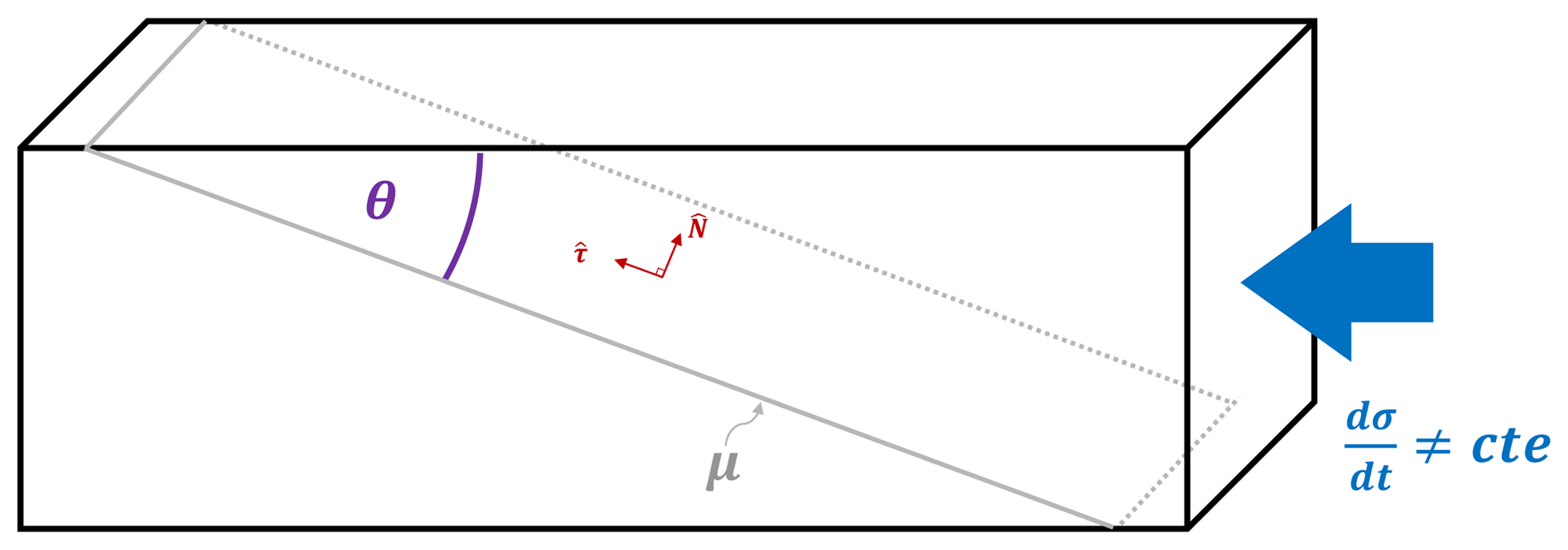
Figure 1Schematic description of the nonconstant uniaxial stresses in presence of a fault with friction coefficient μ and dip angle θ. This schematic description is similar to the experimental setup for pressure stimulated currents (PSC; Kyriazopoulos et al., 2011).

Download

It is possible to relate this shear, and the normal stresses from Eqs. (4)–(5), with the uniaxial stress using the geometry shown in Fig. 1. In this figure, we have a simple schematic representation of the lithosphere under uniaxial stress change dσ∕dt in the presence of a fault with a static friction coefficient μ and a dip angle of 30^∘. We can write this uniaxial stress change in terms of the dip angle θ in the normal and tangential direction (in red on Fig. 1) of the fault, as shown in the following expression:

where dσ∕dt corresponds to the magnitude of uniaxial temporal stress change. Using this expression, we write the brittle–plastic stress contributions in terms of uniaxial stress change as

Substituting Eqs. (2)–(8) into Eq. (1) and considering a second-order linear combination, we obtain the static friction coefficient as a function of time, the fault angle and the semibrittle–plastic changes within the lithosphere given by

where the dots above σ are the notation for the first and second temporal derivative of the uniaxial stress. According to Venegas-Aravena et al. (2019), the temporal stress change $\dot{\mathit{\sigma }}$ has approximately a sigmoidal shape, which can be written as $\dot{\mathit{\sigma }}\left(t\right)=a/(b+e^{(t_{\mathrm{0}}-t)\times w})$, where a, b, w and t₀ are constants. In Fig. 2 we represent $\dot{\mathit{\sigma }}$ and $\ddot{\mathit{\sigma }}$ as a function of time where we have used $a=b=w=\mathrm{1}$ and t₀=10 a.u. (arbitrary units). According to De Santis et al. (2019b), most of the earthquakes recorded occurred close to the center of Fig. 2, which is when t_EQ=t₀. For instance, Marchetti and Akhoondzadeh (2018) have shown that the M_w 8.2 2017 Chiapas (Mexico) earthquake occurred after this time (t_EQ>t₀). They also use daily values of magnetic anomalies ($B\propto \mathrm{d}\mathit{\sigma }/\mathrm{d}t$, which comes directly from the experimental equation $I={\mathit{\alpha }}_{\mathrm{0}}\mathrm{d}\mathit{\sigma }/\mathrm{d}t$, where I is the electric current and α₀ is a constant of proportionality; see Vallianatos and Triantis, 2008, and references therein), thus δt=1 d =86 400 s.

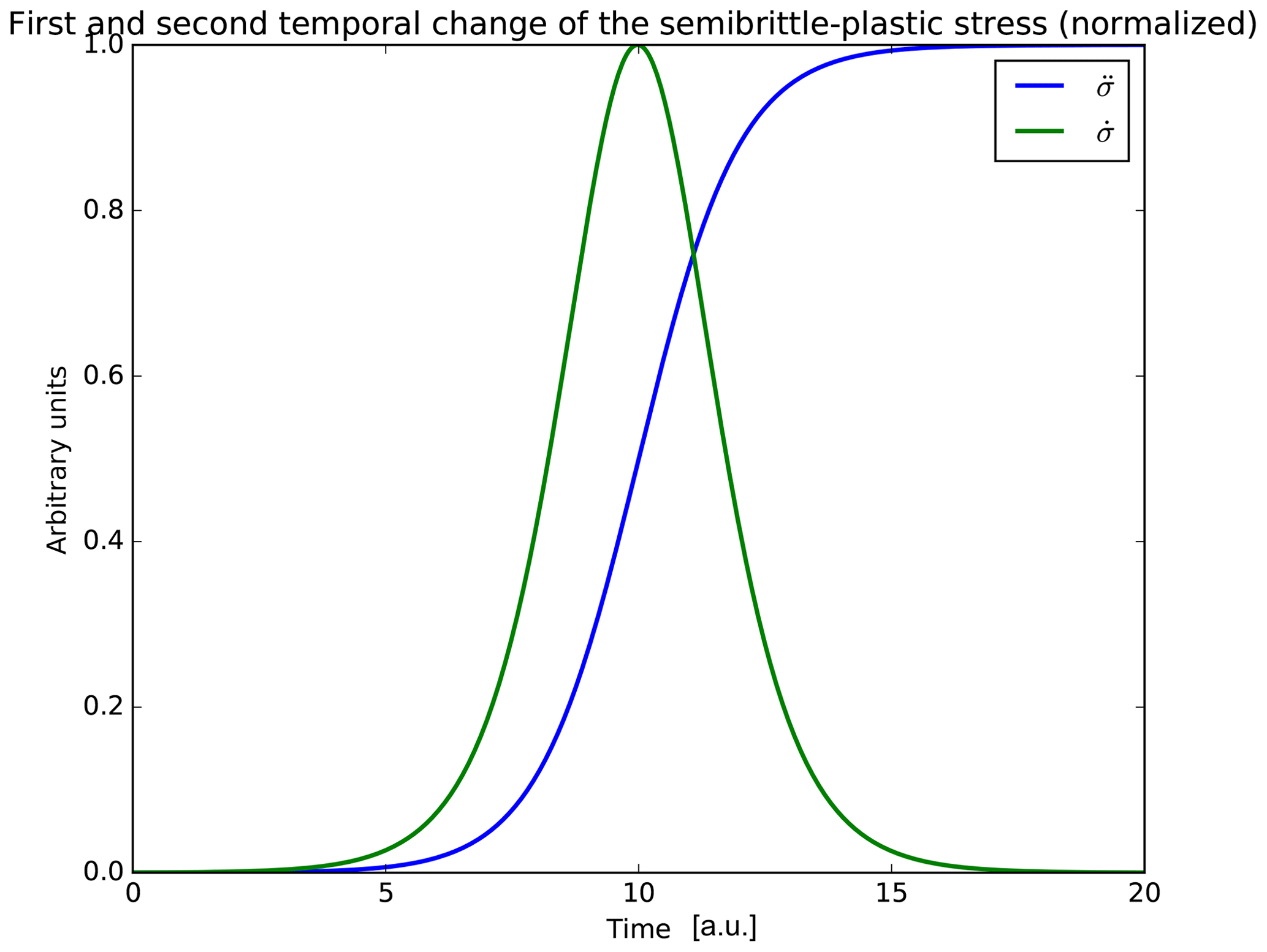
Figure 2Dimensionless representation of normalized first and second temporal change in the uniaxial stress used by Venegas-Aravena et al. (2019). According to De Santis et al. (2019a) the earthquakes occur close to the center of figures. Here it is when $t=t_{\mathrm{0}}=\mathrm{10}$ a.u.

Download

Let us now estimate the values of the constants of Eq. (9). First, we consider the dip or subduction angle θ. According to Maksymowicz (2015), this angle is close to 20^∘ at the depth (∼30 km) and location (35^∘54^′32^′′ S, 72^∘43^′59^′′ W) of the 2010 Maule earthquake. Maksymowicz (2015) claimed that the static friction coefficient in the Chilean convergent margin is close to μ_ch≈0.5. Lamb (2006) calculated that the initial value of τ₀ is 15.4 MPa (constant) in southern Chile. Using μ_ch, it is expected that N₀ should be approximately equal to 30.8 MPa (constant).

In addition, rock experiments show that the values of $\dot{\mathit{\sigma }}$ are close to 1 MPa s⁻¹ (e.g., Saltas et al., 2018). This implies that $\left|k_{\mathrm{1}}\right|$ and $\left|k_{\mathrm{3}}\right|$ must be close to $\sim {\mathrm{10}}^{-\mathrm{4}}$, in order to balance the δt factor. The values of k₂ and k₄ must be equal to or less than $\sim {\mathrm{10}}^{-\mathrm{9}}$, otherwise the values of the friction coefficient would be greater than 1. If we consider an initial increase in the normal stress, the sign of the constants should be negative for k₃, k₄ and positive for k₁, k₂. In Fig. 3 we can see how the friction coefficient changes in time, when using values of k₁ and k₃ described above and different values of k₂ and k₄ (second-order contribution). When we use values on k₂ and k₄ of the order of $\sim {\mathrm{10}}^{-\mathrm{9}}$, it is possible to observe how the friction decreases after the earthquake. Furthermore, it is important to note that the earthquake does not occur when the friction has its maximum value but when it is close to its maximum. When we use values of k₂ and k₄ that are similar or less than $\sim {\mathrm{10}}^{-\mathrm{10}}$, the contribution of $\ddot{\mathit{\sigma }}$ in Eq. (9) vanishes.

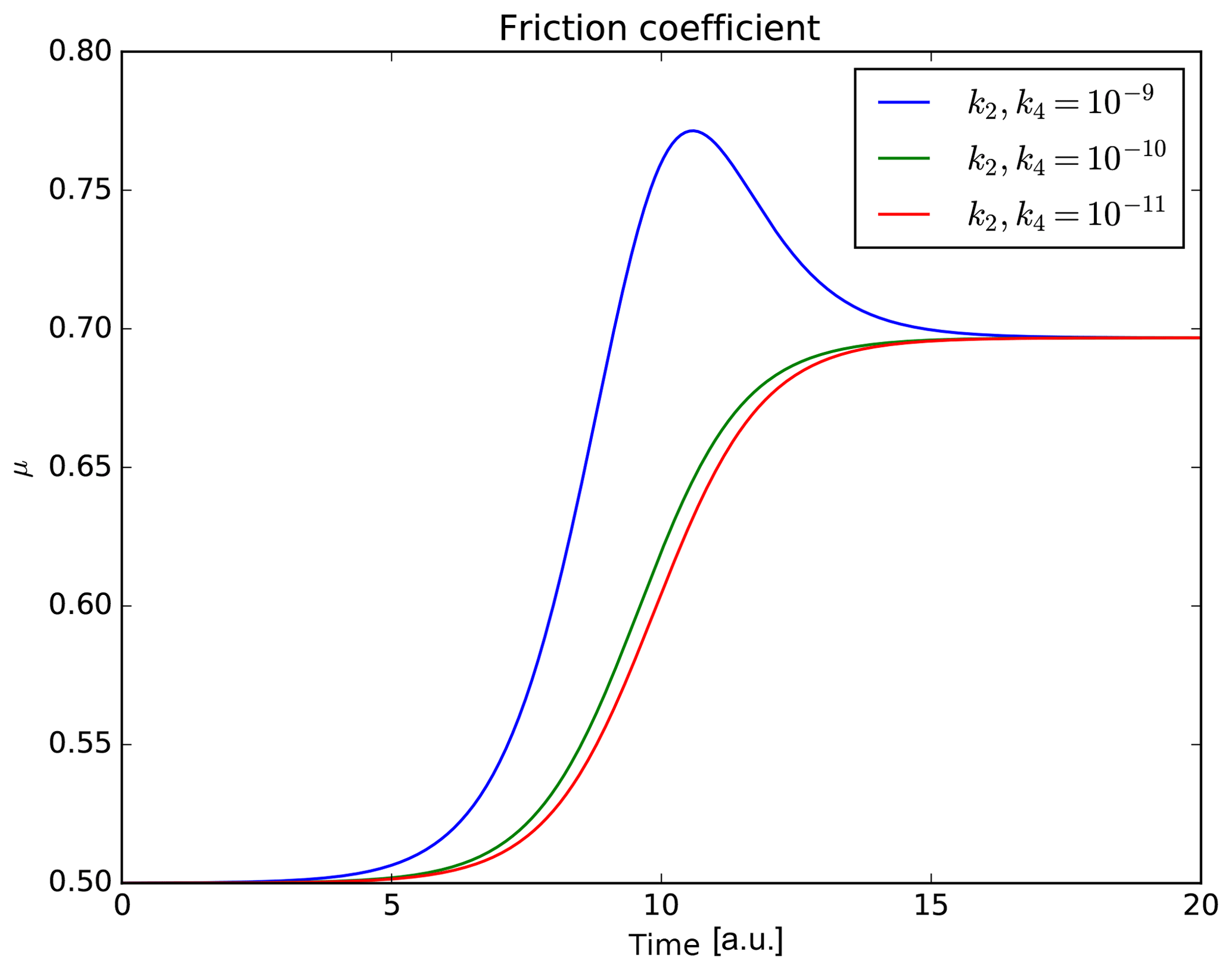
Figure 3Temporal behavior of the semibrittle–plastic friction coefficient using different parameters. In all the cases it is possible to observe an increase in the friction before earthquake (t=10 a.u.). However, the friction decreases after the earthquake only if k₂ and k₄ have values of $\sim {\mathrm{10}}^{-\mathrm{9}}$.

Download

Another critical point is related to the differential time. For instance, when we consider δt≤1 s, the semibrittle–plastic stress term vanishes and the usual friction is recovered. This fact is especially relevant because the semibrittle–plastic contribution to the friction coefficient seems to be relevant only on large timescales. To summarize, the friction coefficient of Eq. (9) could be seen as a generalization of the standard friction coefficient when large timescales are considered.

In the previous section we linked the friction coefficient to the semibrittle–plastic regime that generates microcracks and electrification within the rocks. An important caveat is that this phenomenon does not occur everywhere. For instance, Dobrovolsky et al. (1979) described a specific “preparation zone” required close to the future hypocenter in order to accumulate sufficient stress to trigger the earthquake. This criterion has been widely used by researchers to establish a threshold for determining where the magnetic measurements can be associated with earthquakes (e.g., De Santis et al., 2019a, b). In other words, the phenomenon is local. However, if this is applied, a variation in the friction coefficient related to the rock electrification phenomenon close to the fault would be expected, while a friction variation outside the zones of semibrittle–plastic influence would not.

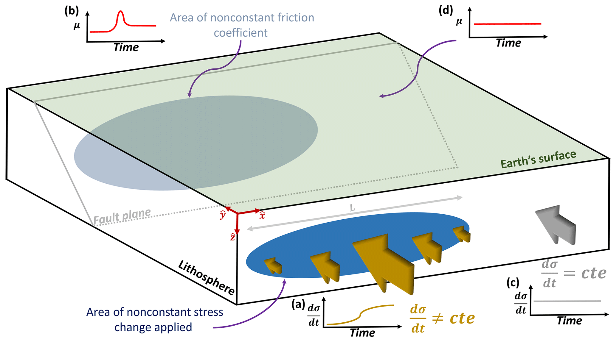
Figure 4Schematic description of friction gradient on the fault. When a constant and nonconstant temporal stress change is applied at different places within the lithosphere, a nonzero friction coefficient gradient is expected.

Download

In order to consider the local variations, we add to our model a separable spatial function of the uniaxial stress as given by $\stackrel{\mathrm{‾}}{\mathit{\sigma }}(x,t)=\mathit{\gamma }\left(x\right)\mathit{\sigma }\left(t\right)$ (for simplicity we choose a uniaxial dependence), where σ(t) corresponds to the same time function as considered in Sect. 2 and γ(x) is the dimensionless spatial distribution parallel to the fault (see the coordinate system in Fig. 4). Let us mention that the values of γ(x) are different when constant and nonconstant stress changes are considered. With this in mind, we can rewrite Eq. (9) as

After straightforward derivations, we get that the gradient of the friction coefficient along the fault using Eq. (10) is given by

where $A=(k_{\mathrm{1}}\dot{\mathit{\sigma }}+k_{\mathrm{2}}\ddot{\mathit{\sigma }}\mathit{\delta }t)\cos \mathit{\theta }\mathit{\delta }t$, $B=(k_{\mathrm{3}}\dot{\mathit{\sigma }}+k_{\mathrm{4}}\ddot{\mathit{\sigma }}\mathit{\delta }t)\sin \mathit{\theta }\mathit{\delta }t$, $\mathit{\alpha }=N_{\mathrm{0}}{k}_{\mathrm{1}}\cos \mathit{\theta }+{\mathit{\tau }}_{\mathrm{0}}{k}_{\mathrm{3}}\sin \mathit{\theta }$ and $\mathit{\beta }=N_{\mathrm{0}}{k}_{\mathrm{2}}\cos \mathit{\theta }+{\mathit{\tau }}_{\mathrm{0}}{k}_{\mathrm{4}}\sin \mathit{\theta }$. Equations (10) and (11) imply that, if we distribute the constant and nonconstant temporal stress change in a nonuniform manner along the fault, then it could be said that this phenomenon is local. This can be understood using the example of Fig. 4: Fig. 4a shows a blue area of length L where we have a nonconstant temporal stress change. There one observes a change in the friction coefficient inside the projected gray area (Fig. 4b). Conversely, outside the area of length L (Fig. 4c), we assume a constant stress change, and there is no change in the friction coefficient (Fig. 4d). Let us remind ourselves that the entire fault suffered from stress accumulation during the entire process. However, only the gray area is directly affected by the friction change. This shows that the temporal friction changes are restricted only to a specific area (gray area) on the fault. Hence, one observes a nonzero friction coefficient gradient on the fault and we have a local phenomenon ($\mathrm{\nabla }\stackrel{\mathrm{‾}}{\mathit{\mu }}\ne \mathrm{0}\iff \mathrm{Local}$).

The process described in Fig. 4 reveals why the magnetic measurements are not global. It also validates the locality criteria in terms of fault properties. Furthermore, the spatial distribution of magnetic field measurements is expected to have a length scale comparable to the friction coefficient change due to the dependency of γ(x) in Eq. (10). That is, the larger the detection area of magnetic anomalies, the larger the area where fault friction is changing. In addition, Venegas-Aravena et al. (2019) described how the uniaxial stress change implies a change in the b-value of the Gutenberg–Richter law. It also implies that a significant earthquake is needed in order to satisfy this change in the Gutenberg–Richter law. Therefore, a greater expected magnitude could be related to changes in the coefficient of friction within an area within the fault. However, changes in the friction coefficient do not directly imply the earthquakes generation itself.

Up to this point, no changes in the elastic stresses have been considered in Eq. (10). This section focuses on one of the elastic parameter that is involved in the seismic rupture process: the stress drop Δτ. This parameter is one of the most relevant because it shows the shear stress differences prior to and after the onset of the earthquake within the fault rupture area (e.g., Aki, 1966). Furthermore, this parameter is also related to the seismic waves radiated (through the corner frequency of waves) and the seismic moment M₀ (e.g., Eshelby, 1957; Brune, 1970; Baltay et al., 2011, and references therein). If we consider a circular rupture area with radius d_crack, the stress drop Δτ is linked with the seismic moment M₀ through the following equation (Eshelby, 1957).

On the other hand, the seismic moment M₀ and the moment magnitude M_w in terms of the coseismic magnetic field are also related. Hence, the seismic moment is given by

where μ_sm is the shear modulus, d the average slip, D the fractal dimension of rock and B_cs the coseismic magnetic field; J corresponds to the total electric current density; μ_m is the magnetic permeability of the medium; r is the distance to the fault; l_max and l_min are the radius of the circular rupture area and the smallest microcrack length, respectively. The circular rupture is calculated using $l_{max}=\sqrt{S/\mathit{\pi }}$, where S corresponds to the total rupture area.

In this case, the rupture geometry is circular in both formulations, thus, $d_{\mathrm{crack}}=l_{max}$. Substituting this into Eqs. (13) and (12) we obtain

Equation (14) relates the stress drop with the coseismic magnetic field, seismic rupture, and the electrical and mechanical properties of rocks (lithosphere). We can use the data from the Maule earthquake in order to compare the result of Eq. (14) with those found by other researchers. If we use the fault values ${\mathit{\mu }}_{\mathrm{sm}}=\mathrm{3.3}\times {\mathrm{10}}^{\mathrm{10}}$ Pa, d=4 m and $S=\mathrm{450}\times \mathrm{120}$ km² (Vigny et al., 2011; Yue et al., 2014); the granite rock and brittle properties ${\mathit{\mu }}_{\mathrm{m}}=\mathrm{13.5}\times {\mathrm{10}}^{-\mathrm{7}}$ N A⁻² (Scott, 1983), $J=\mathrm{5}\times {\mathrm{10}}^{-\mathrm{6}}$ A m⁻² (Tzanis and Vallianatos, 2002), $l_{min}={\mathrm{10}}^{-\mathrm{3}}$ m (Shah, 2011) and D=2.6 (Turcotte, 1997); and the magnetic data B_cs≈0.1 nT at r≈250 km (Fig. 5 in Venegas-Aravena et al., 2019), we obtain a stress drop Δτ≈3.4 MPa. This result is in close agreement with the result of Luttrell et al. (2011; 4 MPa). Using this value, we can calculate the elastic shear stress as

where H(t−t₀) corresponds to the step function centered at t₀ (the moment of the earthquake occurrence) and γ₂ is a dimensionless second step function that represents the fault area where the stress drop exists. This means that γ₂=0 outside the rupture area and γ₂=1 if the point is within the rupture area. Combining this result into Eq. (10), we calculate the total friction coefficient ${\stackrel{\mathrm{‾}}{\mathit{\mu }}}_{\mathrm{T}}$ of the fault as

This total friction coefficient ${\stackrel{\mathrm{‾}}{\mathit{\mu }}}_{\mathrm{T}}$ is especially relevant because of the dependence of the coseismic magnetic field B_cs (through the stress drop Δτ) and the magnetic anomalies (through the relation $B\propto \dot{\mathit{\sigma }}$). Furthermore, Eq. (16) explains the spatial distribution of friction along the fault in addition to its time variations. In Eq. (16), the spatial changes in friction (represented by γ) are not necessarily related to the seismic rupture area (represented by γ₂). However, in the case where they are related, one expects γ₂ to be a function of γ. That is γ₂=γ₂(γ(x)). In the general case the total friction coefficient gradient can be written as

where $\mathrm{\Gamma }(\mathit{\gamma },{\mathit{\gamma }}_{\mathrm{2}})=\mathrm{1}/(N_{\mathrm{0}}-\mathit{\gamma }B{)}^{\mathrm{2}}[{\mathit{\gamma }}_{\mathrm{2}}^{\prime }(\mathit{\gamma }B-N_{\mathrm{0}})-{\mathit{\gamma }}^{\prime }{\mathit{\gamma }}_{\mathrm{2}}B]$, $\mathrm{\nabla }\stackrel{\mathrm{‾}}{\mathit{\mu }}$ is the friction gradient already defined in Eq. (11), and the same definitions for A and B are used. The second term of Eq. (17) implies that a more complex spatial friction distribution on the fault is expected after the earthquake. When no brittle–plastic contribution is considered (γ=0), the friction is only proportional to the gradient of fault rupture distribution ($\mathrm{\nabla }{\stackrel{\mathrm{‾}}{\mathit{\mu }}}_{\mathrm{T}}=-\mathrm{\Delta }\mathit{\tau }H(t-t_{\mathrm{0}}){\mathit{\gamma }}_{\mathrm{2}}^{\prime }/N_{\mathrm{0}}$). When γ₂≈γ, the two terms of the total friction coefficient will be proportional to the spatial distribution gradient ($\mathrm{\nabla }{\stackrel{\mathrm{‾}}{\mathit{\mu }}}_{\mathrm{T}}\propto {\mathit{\gamma }}^{\prime }$). If the earthquake does not occur, the second term vanishes and Eq. (11) is recovered.

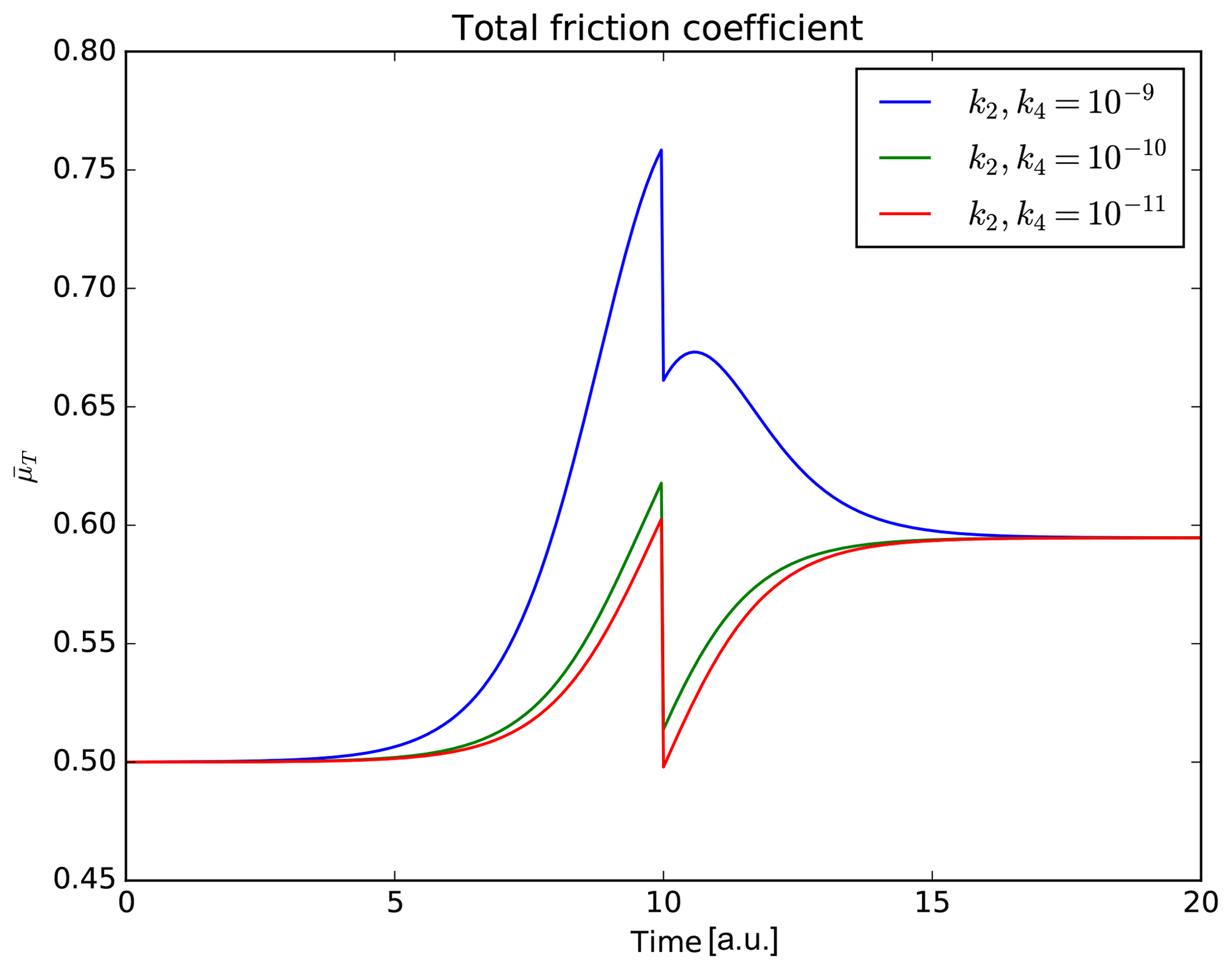
Figure 5Total fiction coefficient from the seismo-electromagnetic theory derivation. If we consider one point within the rupture area, the highest values of friction are found before the earthquake (t=10 a.u.). The friction decreases at t=10 a.u. was calculated using the stress drop as a function of the coseismic magnetic field. The maximum value is not completely recovered after the earthquake occurs.

Download

As an illustration, if we consider one point affected by the rupture area and the same values as in Fig. 3, we can calculate the shape of the total friction coefficient as shown in Fig. 5. The three cases show an increase in the friction coefficient prior to the earthquake, and in the three cases the friction reaches its maximum values before the earthquake (at t=10 a.u.). The subsequent decrease is due to the stress drop influence calculated using the coseismic magnetic field B_cs. After the earthquake, in none of the cases is the friction completely recovered to its values before the earthquake.

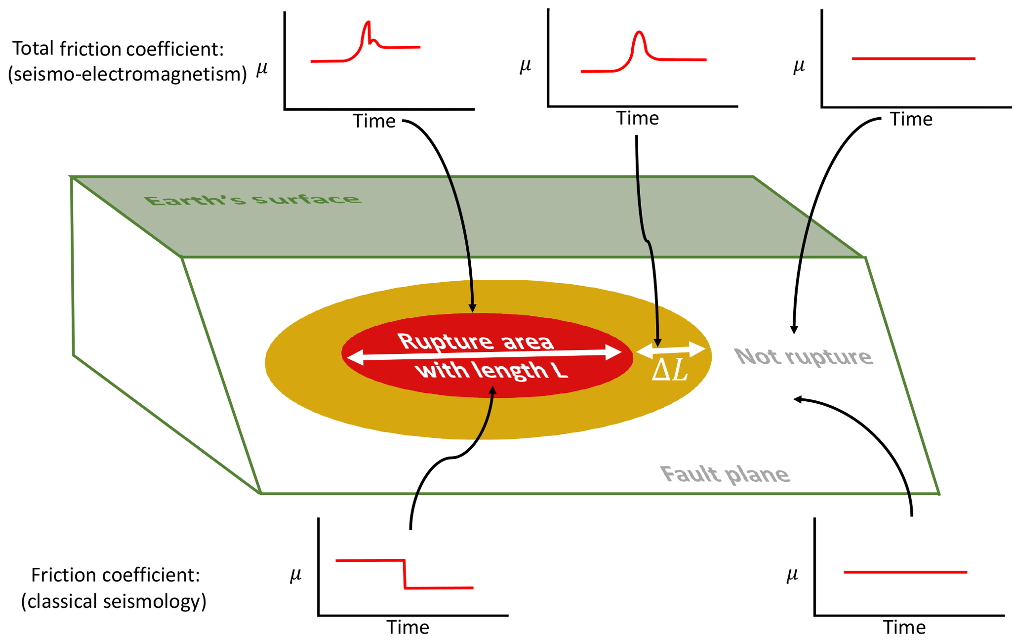
Figure 6Schematic comparison among different friction behaviors related to seismic rupture area. At the top the result of friction in the context of the seismo-electromagnetic theory is presented. At the bottom the classical view of the friction is presented. When the rupture occurs, a friction drop is observed in the two theories. However, a friction increase exists in the case studied in this work.

Download

As a second illustration, it is also possible to compare the temporal behavior of the friction coefficient at different points within the fault. For instance, in Fig. 6 (top) we show the different friction behaviors expected if we consider the total friction coefficient. The red area indicates the area where the friction drop occurs. A friction drop is not expected to occur outside the red zone. However, it is possible to observe differences in the coefficient of friction close to the rupture zone where γ₂≠γ (yellow area). In both the rupture zone and its surroundings (marked as red and yellow areas, respectively, in Fig. 6) there are changes in the coefficient of friction prior to the rupture. In stark contrast, the standard friction drop is expected only in the rupture zone (red area) and a nonmeasurable change in friction is expected prior to the earthquake (Fig. 6, bottom).

We can summarize our analysis by using two different distributions of γ and γ₂. For instance, in Fig. 7 we show the double-sigmoidal distribution for γ and γ₂ (black and red curves, respectively) along the fault x direction (of total length 2x_half). The dimensionless distribution is defined as a combination of the sigmoidal function used in Sect. 2 as

If we consider $a=b=\mathrm{1}$ and x_half=10 a.u. in both distributions; x₀=5 a.u., L=10 a.u. and w=1 a.u. for γ; and x₀=8 a.u., L=4 a.u. and w=10 a.u. for γ₂, we get the two distributions of Fig. 7. These values indicate the same situation as discussed in Fig. 6, that is a rupture length (L=4 a.u. in γ₂ represents the x direction of the red area in Fig. 6) influenced less by the friction coefficient than by semibrittle–plastic stress (here L=10 a.u. in γ represents the x direction of the yellow area in Fig. 6). Using both sets of values, those used in the stress drop (Eq. 14) and also the same k parameters used in Eq. (9), we calculate the total friction coefficient (Eq. 16) as shown in Fig. 8 (case $k_{\mathrm{2}}=k_{\mathrm{4}}={\mathrm{10}}^{-\mathrm{9}}$). At time t=0 a.u., no friction changes occur (${\stackrel{\mathrm{‾}}{\mathit{\mu }}}_{\mathrm{T}}=\mathrm{0.5}$). However, the friction increases at t=5 a.u., where the spatial distribution γ is initially defined as nonzero ($x\in [\mathrm{5},\mathrm{15}]$ a.u.). The friction increases up to t=10 a.u., the time corresponding to the earthquake occurrence. The earthquake rupture length is shown as a sudden friction decrease ($x\in [\mathrm{8},\mathrm{12}]$ a.u.) from 0.76 to 0.67. In the zone immediately next to the rupture, the friction increases even more up to the maximum values (0.77), while in the rupture section the friction decreases. After this time (t∼12 a.u.), the rupture and the surrounding section experience a friction decrease.

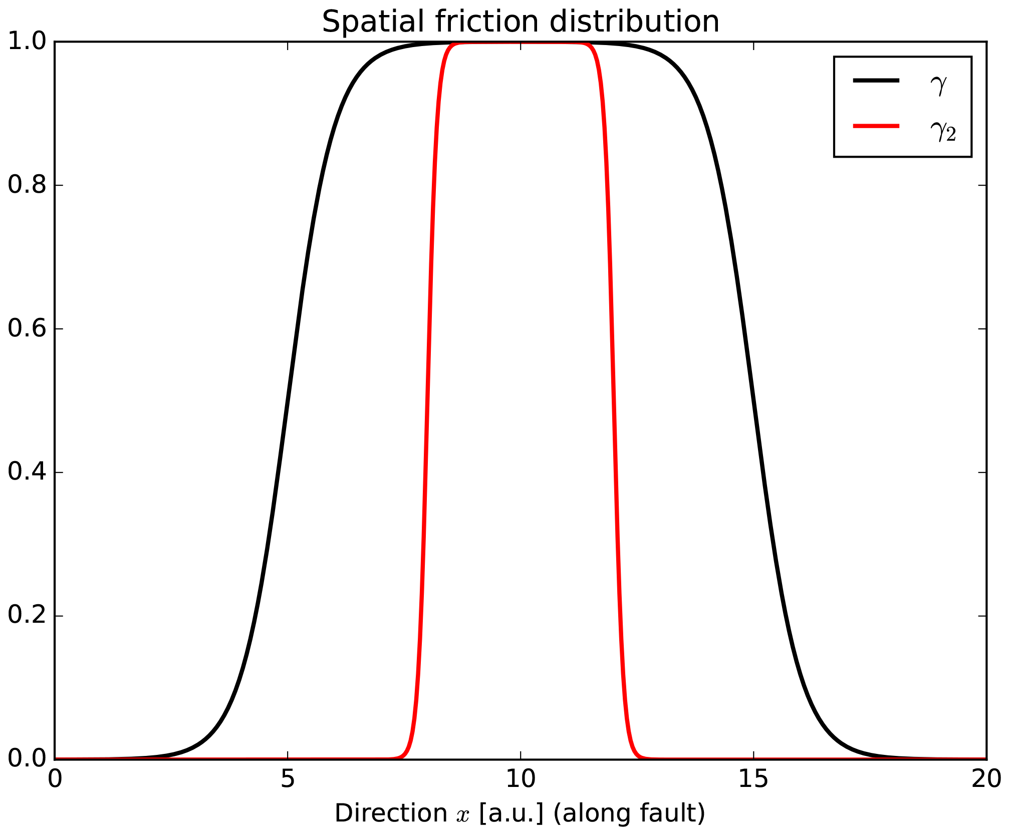
Figure 7Spatial distribution of γ and γ₂. These functions represent the different sections (or behavior) of friction on the fault along the x direction. The distribution γ₂ represents the stress drop section and distribution γ represents the semibrittle–plastic influence region.

Download

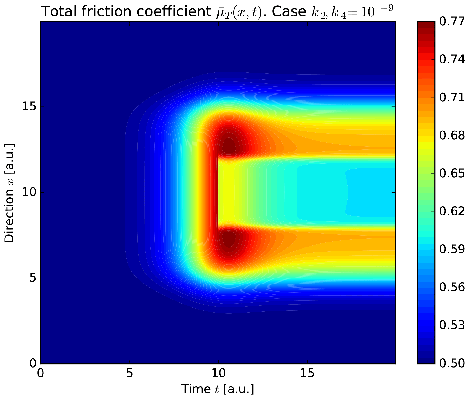
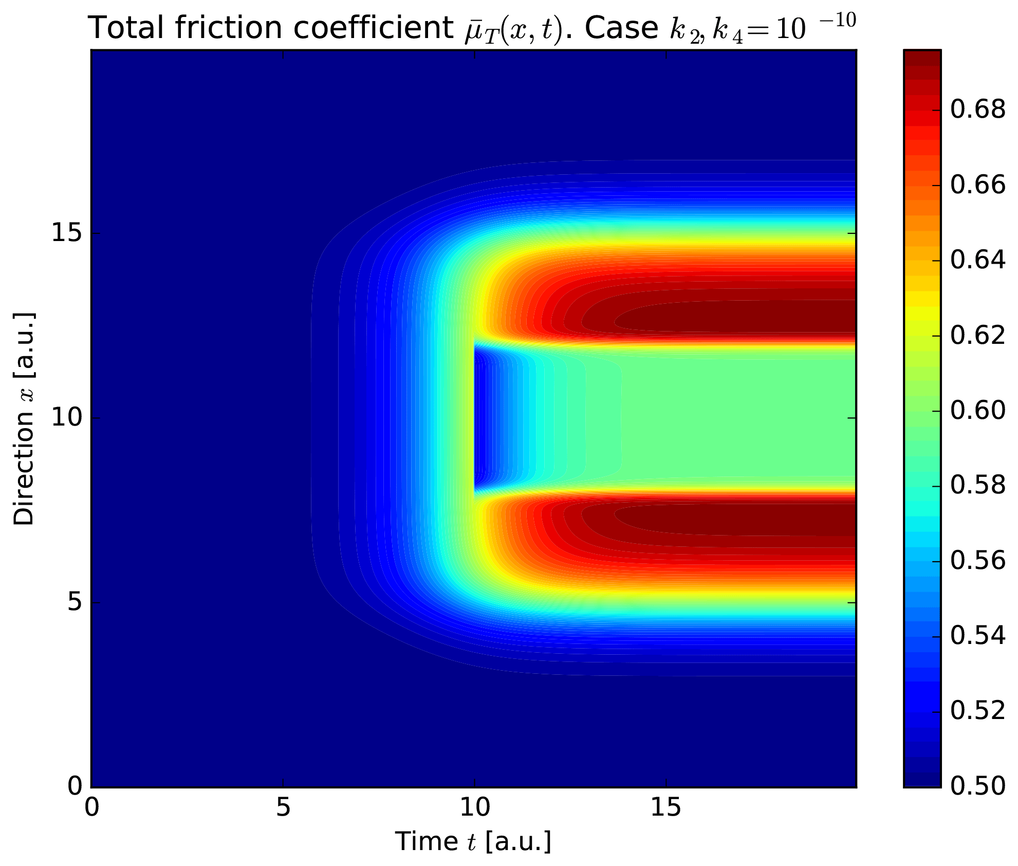
Figure 8Spatial–temporal total friction coefficient ${\stackrel{\mathrm{‾}}{\mathit{\mu }}}_{\mathrm{T}}(x,t)$ along the fault x direction using $k_{\mathrm{2}}=k_{\mathrm{4}}={\mathrm{10}}^{-\mathrm{9}}$. The righthand color bar indicate the friction coefficient values at a certain time and position. The earthquake occurs when t=10 a.u. At this time, the stress drop (defined by the distribution γ₂) $\mathrm{\Delta }\mathit{\tau }\in [\mathrm{8},\mathrm{12}]$ a.u.

Download

The case of $k_{\mathrm{2}}=k_{\mathrm{4}}={\mathrm{10}}^{-\mathrm{10}}$ is shown in Fig. 9. The rupture is shown as a blue area at t=10 a.u. in section $x\in [\mathrm{8},\mathrm{12}]$ a.u. At this time and location, we observe that the friction decreases to similar initial values (∼0.5). The friction of this rupture section increases after the earthquake up to ∼0.6. On the other hand, the rupture's surrounding section increases up to the maximum values (∼0.7). Despite those facts, the initial (t=0 a.u.) and final (t=20 a.u.) friction values are almost identical for both cases. For instance, the rupture area has values close to 0.6 in Figs. 8 and 9. The surrounding rupture section has values close to 0.69 in both cases, and the section away from the rupture (close to x=0 a.u. and x=20 a.u.) always has the same initial value (0.5) in both cases. However, both cases exhibit a complex time behavior after the earthquake occurrence, as Eq. (17) indicates.

Figure 9Same spatial–temporal total friction coefficient as in Fig. 8 but using k₂, $k_{\mathrm{4}}={\mathrm{10}}^{-\mathrm{10}}$.

Download

Finally when the semibrittle–plastic contribution is not considered, we get that γ=0. The result is shown in Fig. 10 and is only observed with the sudden friction decrease at t=10 a.u. (and $x\in [\mathrm{8},\mathrm{12}]$ a.u.). In this later case none of the other complex friction behaviors is observed.

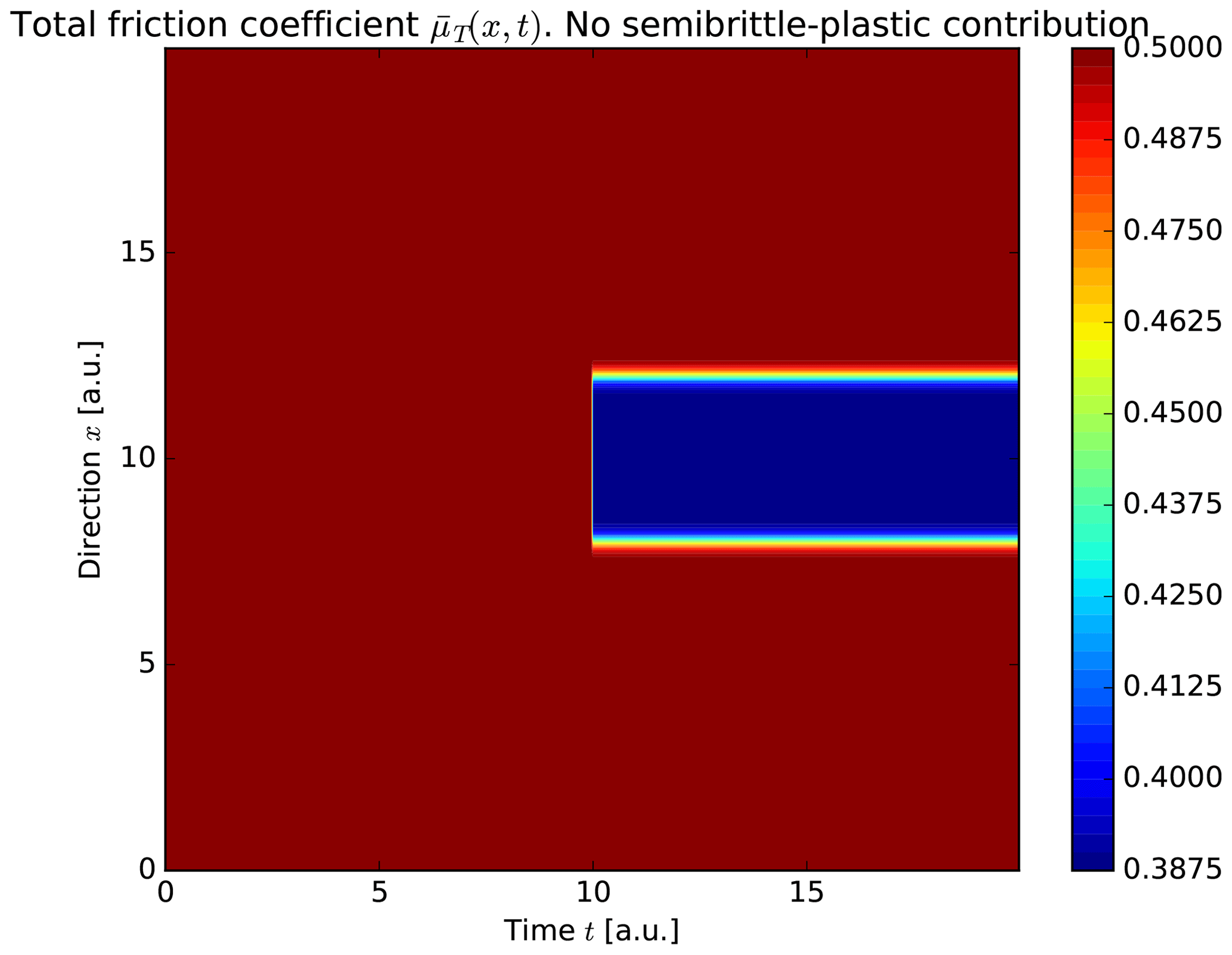
Figure 10Total friction coefficient using no semibrittle–plastic contribution. That is γ(x)=0, $\forall x\in [\mathrm{0},\mathrm{2}{x}_{\mathrm{half}}]$. The friction variation exists only when the earthquake occurs (t=10 a.u.) and at the earthquake rupture place ($\mathrm{\Delta }\mathit{\tau }\in [\mathrm{8},\mathrm{12}]$ a.u. in this case).

Download

A general expression for friction has been obtained in Eq. (16). Following this we can adapt the Gutenberg–Richter law in this semibrittle–plastic context. Let us remind ourselves that this law establishes a relation between the number of earthquakes in a region and their magnitude (Gutenberg and Richter, 1944). Mathematically, this link is written as $\log N=a-b\times m$, where N is the number of earthquakes with magnitude equal to or greater than m and a and b are constants. However, the b-value of this law might evolve in time. Indeed, De Santis et al. (2011) determined an equation that relates the temporal evolution of the parameter b (b=b(t)) and the measure of the entropy (stress) H(t) of that region as $b\left(t\right)=b_{max}{\mathrm{10}}^{-H\left(t\right)}$, where $b_{max}=e{\log }_{\mathrm{10}}e$. The entropy H(t) is assumed to be proportional to the real stress in the lithosphere (Venegas-Aravena et al., 2019). If we consider the total shear stress τ_T in the fault described by Eq. (16), we can write

where ${\mathit{\tau }}_{\mathrm{T}}={\mathit{\tau }}_{\mathrm{0}}-{\mathit{\gamma }}_{\mathrm{2}}\mathrm{\Delta }\mathit{\tau }H(t-t_{\mathrm{0}})+\mathit{\gamma }(k_{\mathrm{1}}\dot{\mathit{\sigma }}+k_{\mathrm{2}}\ddot{\mathit{\sigma }}\mathit{\delta }t)\cos \mathit{\theta }\mathit{\delta }t$ and k₀ is a constant with dimensions of an inverse stress. If we use the same values as in Fig. 5 ($k_{\mathrm{2}}=k_{\mathrm{4}}={\mathrm{10}}^{-\mathrm{9}}$), we get the temporal evolution of the b-value (Fig. 11a). Figure 11a shows a decrease in the b-value until the earthquake occurs (at t=10 a.u.). Figure 11b shows the Gutenberg–Richter law at three instants of time (and k₀=0.01, a=1): initial (t=0 a.u.), prior to the earthquake (t=9 a.u.) and final (t=20 a.u.). This figure shows how large earthquakes (M_w∼6) are not expected at the initial moment (blue line). However, just before the earthquake, an M8-class earthquake should be expected (green line). After the earthquake one would only expect earthquakes no greater than M_w∼7 to exist (red line). Figure 12a and b show the same previous case but now considering $k_{\mathrm{2}}=k_{\mathrm{4}}={\mathrm{10}}^{-\mathrm{10}}$. In this case there is no difference between time immediately before the earthquake (t=9 a.u.) and at the final time (t=20 a.u.). In addition, using these parameters ($k_{\mathrm{2}}=k_{\mathrm{4}}={\mathrm{10}}^{-\mathrm{10}}$), smaller magnitudes are reached than when using $k_{\mathrm{2}}=k_{\mathrm{4}}={\mathrm{10}}^{-\mathrm{9}}$ (M_w∼7 and M_w∼8, respectively). This is why it is more likely that earthquakes of greater magnitude will be found when considering the contribution of the $\ddot{\mathit{\sigma }}$ term in the analysis.

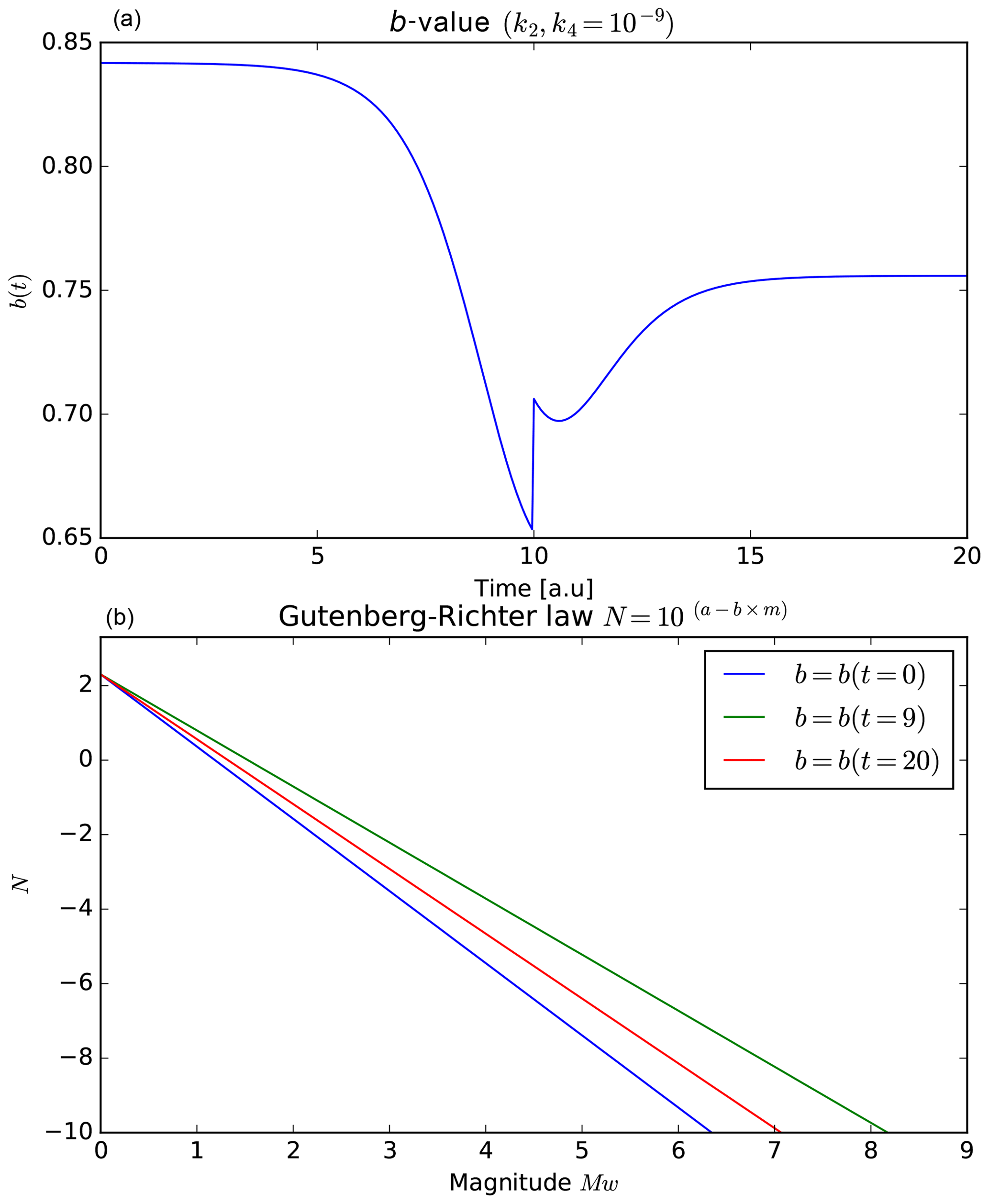
Figure 11(a) The b-value using σ=ατ; $k_{\mathrm{2}}=k_{\mathrm{4}}={\mathrm{10}}^{-\mathrm{9}}$ and α=0.01. (b) The Gutenberg–Richter law for instants of time t=0 a.u., t=9 a.u. and t=20 a.u. The b-value decreases before the earthquake implying stronger seismic events.

Download

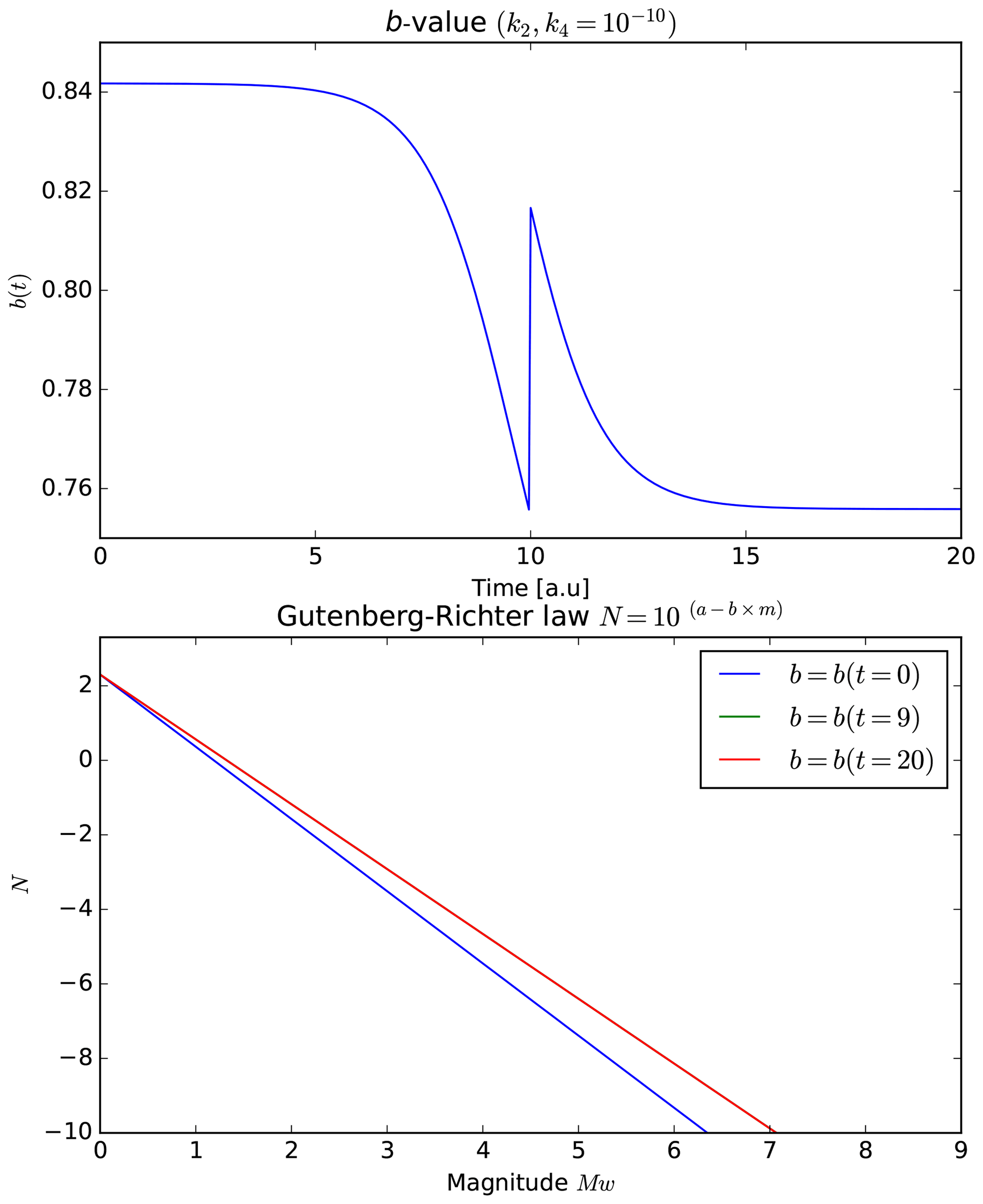
Figure 12The b-value and Gutenberg–Richter law using $k_{\mathrm{2}}=k_{\mathrm{4}}={\mathrm{10}}^{-\mathrm{10}}$. The green and red curves are the same.

Download

In Sect. 5 we determine that $k_{\mathrm{2}}=k_{\mathrm{4}}={\mathrm{10}}^{-\mathrm{9}}$ were the most adequate values. Despite this fact, the Gutenberg–Richter law does not provide an approximate time t₀ for the earthquake occurrences. If we look at Eq. (16), the term t₀ appears explicitly (in the step function). However, t₀ appears only after the earthquake, so it is not possible to find t₀ analytically before the rupture (using the rupture itself). This means that we must find an estimate using the other parameters. One way to do it is to consider the differential total friction coefficient $\mathrm{d}{\stackrel{\mathrm{‾}}{\mathit{\mu }}}_{\mathrm{T}}$ to find an approximate rupture time t₀. Figure 13 shows $\mathrm{d}{\stackrel{\mathrm{‾}}{\mathit{\mu }}}_{\mathrm{T}}$ considering ${\mathit{\gamma }}_{\mathrm{2}}=\mathit{\gamma }=\mathrm{1}$, $k_{\mathrm{2}}=k_{\mathrm{4}}={\mathrm{10}}^{-\mathrm{9}}$ and $k_{\mathrm{2}}=k_{\mathrm{4}}={\mathrm{10}}^{-\mathrm{10}}$. When major earthquakes ($k_{\mathrm{2}}=k_{\mathrm{4}}={\mathrm{10}}^{-\mathrm{9}}$) are considered, the rupture occurs after the maximum value ($(\mathrm{d}{\stackrel{\mathrm{‾}}{\mathit{\mu }}}_{\mathrm{T}}{)}_{\mathrm{MAX}}$), when $\mathrm{d}{\stackrel{\mathrm{‾}}{\mathit{\mu }}}_{\mathrm{T}}\approx \mathrm{1}/\mathrm{2}(\mathrm{d}{\stackrel{\mathrm{‾}}{\mathit{\mu }}}_{\mathrm{T}}{)}_{\mathrm{MAX}}$ (Fig. 13, top). When k₂, $k_{\mathrm{4}}={\mathrm{10}}^{-\mathrm{10}}$, the rupture also occurs after the maximum value, in this case $\mathrm{d}{\stackrel{\mathrm{‾}}{\mathit{\mu }}}_{\mathrm{T}}\approx \mathrm{0.9}(\mathrm{d}{\stackrel{\mathrm{‾}}{\mathit{\mu }}}_{\mathrm{T}}{)}_{\mathrm{MAX}}$ (Fig. 13, bottom). Considering these two limiting cases in this framework we conclude that earthquakes occur after ($\mathrm{d}{\stackrel{\mathrm{‾}}{\mathit{\mu }}}_{\mathrm{T}}{)}_{\mathrm{MAX}}$ when the differential total friction coefficient decreases to $\mathrm{d}{\stackrel{\mathrm{‾}}{\mathit{\mu }}}_{\mathrm{T}}\approx C(\mathrm{d}{\stackrel{\mathrm{‾}}{\mathit{\mu }}}_{\mathrm{T}}{)}_{\mathrm{MAX}}$, where $C\in [\mathrm{0.5},\mathrm{0.9}]$.

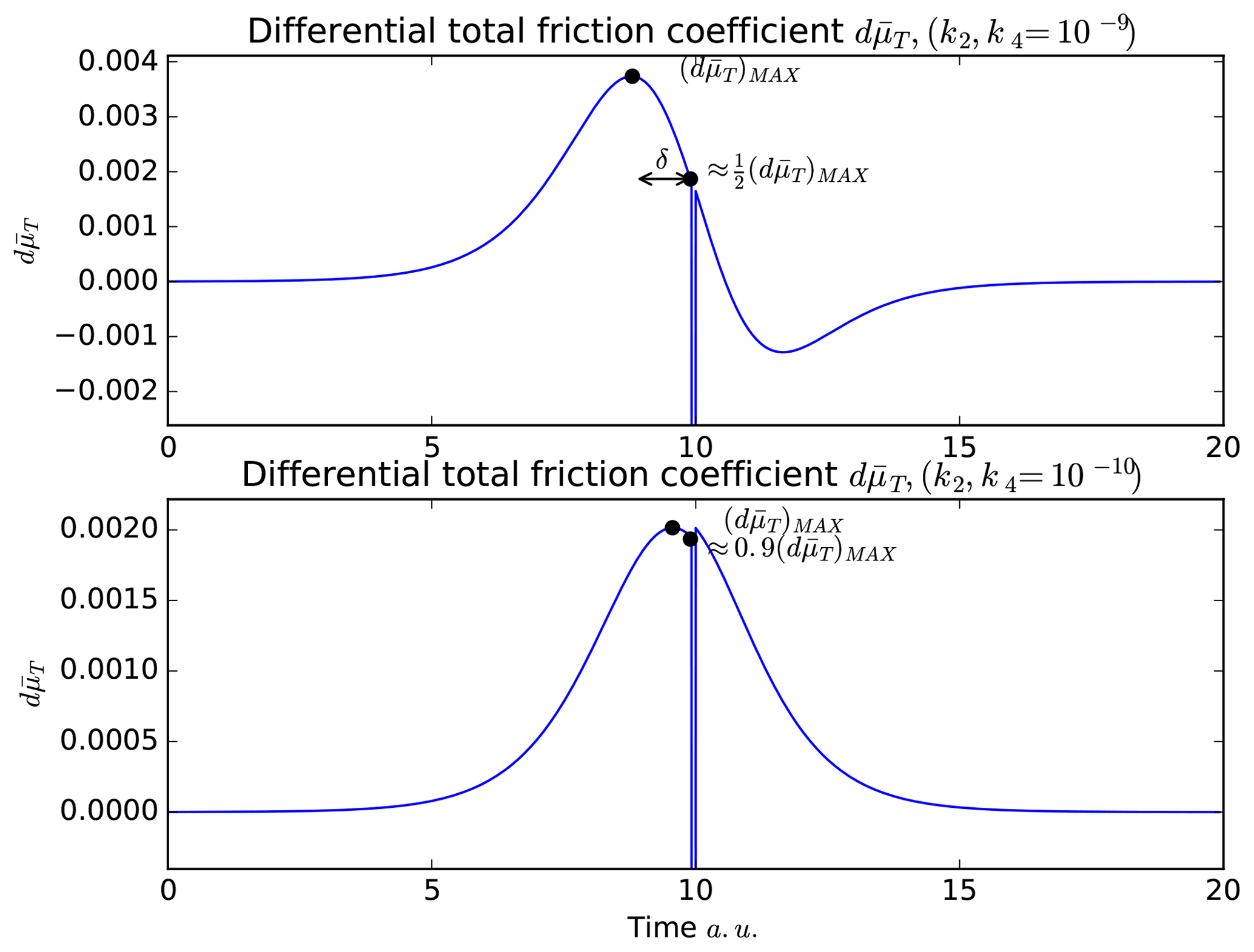
Figure 13Different ruptures times viewed from the differential total friction coefficient $\mathrm{d}{\stackrel{\mathrm{‾}}{\mathit{\mu }}}_{\mathrm{T}}$ and using different values of k₂ and k₄. The rupture occurs after the maximum differential total friction coefficient $(\mathrm{d}{\stackrel{\mathrm{‾}}{\mathit{\mu }}}_{\mathrm{T}}{)}_{\mathrm{MAX}}$, when $\mathrm{d}{\stackrel{\mathrm{‾}}{\mathit{\mu }}}_{\mathrm{T}}$ have values close to 0.5–0.9 times $(\mathrm{d}{\stackrel{\mathrm{‾}}{\mathit{\mu }}}_{\mathrm{T}}{)}_{\mathrm{MAX}}$.

Download

The time between $\mathrm{d}{\stackrel{\mathrm{‾}}{\mathit{\mu }}}_{\mathrm{T}}\approx (\mathrm{d}{\stackrel{\mathrm{‾}}{\mathit{\mu }}}_{\mathrm{T}}{)}_{\mathrm{MAX}}$ and $\mathrm{d}{\stackrel{\mathrm{‾}}{\mathit{\mu }}}_{\mathrm{T}}\approx C(\mathrm{d}{\stackrel{\mathrm{‾}}{\mathit{\mu }}}_{\mathrm{T}}{)}_{\mathrm{MAX}}$ can be denoted by δ. This δ parameter increases when C decreases and vice versa, so δ is inversely proportional to C ($\mathit{\delta }\propto C^{-\mathrm{1}}$). Then, we arrive at an expression for the general rupture time t₀ as follows:

where $t_{(\mathrm{d}{\stackrel{\mathrm{‾}}{\mathit{\mu }}}_{\mathrm{T}}{)}_{\mathrm{MAX}}}$ is the time when $\mathrm{d}{\stackrel{\mathrm{‾}}{\mathit{\mu }}}_{\mathrm{T}}\approx (\mathrm{d}{\stackrel{\mathrm{‾}}{\mathit{\mu }}}_{\mathrm{T}}{)}_{\mathrm{MAX}}$. Note that Eq. (20) is only valid after the maximum value ($\mathrm{d}{\stackrel{\mathrm{‾}}{\mathit{\mu }}}_{\mathrm{T}}{)}_{\mathrm{MAX}}$ is reached. Equation (20) is general; however, considering the Gutenberg–Richter law, we expect that C values close to 0.5 are necessary to represent earthquakes of greater magnitude in this theoretical framework.

All the data are open source and can be found using the references that are listed in the text. The numerical data can be easily generated by everyone using the equations and indications of the text. If you have any problems, do not hesitate to write and ask the authors.

PVA conceived the theoretical derivation and numerical implementation. PVA also performed the initial paper writing and created the figures. EGC and DL carried out the writing corrections and generated the scientific view, background and support.

The authors declare that they have no conflict of interest.

This research has been partially supported by Centers of Excellence with CONICYT Basal (grant no. AFB180001, CEDENNA).

This paper was edited by Filippos Vallianatos and reviewed by Angelo De Santis and Michael E. Contadakis.