2.1 The empirical spatial extremogram (ESE)

The objective of the present section is to use an approach based on the spatial extremogram to form a homogenous region to be used in a RFA of extreme SSSs. The region of interest which is expected to be centered on a given target site must be physically and statistically homogeneous. The use of the spatial extremogram technique in index-flood-based RFA is the main contribution of the present paper. It is expected that the spatial-extremogram-based procedure leads to regions of interest with no border effect and with less residual heterogeneity.

Let X and Y be the random explanatory variables of the SSSs at sites S₁ (the target site) and any other site S₂, respectively. Let q₁ and q₂ be the two samples extreme quantiles (thresholds above which SSSs are considered to be extremes) for sites S₁ and S₂, respectively. Site S₂ is inside the physically homogeneous region centered on the target site S₁ if, at least, a certain part of extreme SSSs from each site are likely to be simultaneously induced by the same storms. This means that there is an extremal dependency between both sites. In the spatial and pairwise dependence description the temporal dimension should be included because storm conditions can last several days. The ESE computation is then based on the pairwise extremal dependences (between any site and the target site), and it can be defined by the spatial extremal coefficient ρ(X, Y), as proposed by Hamdi et al. (2016), and expressed as

The empirical and spatial extremal coefficient is the natural estimator $\widehat{\mathit{\rho }}$ of ρ, and it is defined by

where I{f} is equal to 1 if f is true, and to 0 otherwise, N is the number of extreme events X(t)>q₁ at the target site (events that exceeded the sample extreme quantile q₁), and D is the number of overlapped extreme twins $X\left(t\right)>q_{\mathrm{1}}\mathit{\&}Y\left(t\right)>q_{\mathrm{2}}$, extreme events generated by the same storm that occurred at sites S₁ and S₂. It was considered that two observations were generated by the same storm if the time difference between their two moments of occurrence was less, in absolute value, than 6 h (other durations were tested, 12 and 24 h, but the results were similar). It is noteworthy that D must be large enough in order for the ESE computation to be reliable. Indeed, the larger it is, the more significant the probability of extremal dependence. The fact that $\widehat{\mathit{\rho }}(X$, Y) ranges between 0 and 1 indicates the existence of a certain extremal dependency between X and Y. The higher the empirical extremal coefficient $\widehat{\mathit{\rho }}$, the stronger the dependency is between both sites. Indeed, we obtain an extremal coefficient equal to 1 in the case of perfect dependency between sites (theoretically, this can only happen when computing the extremal dependency between a site and itself). But more interestingly, $\widehat{\mathit{\rho }}$ is relatively high when a storm is observed at site S₁; thus, relatively often, this storm is also observed at site S₂. However, the extremal coefficient tends towards 0 when the site of interest is far enough from the target site. In other words, the observations at sites, generally widely separated geographically, can be considered to be asymptotically independent. An illustrative example on how the extremal dependence coefficient is empirically computed is presented in Fig. 1. As is shown in this example, among the seven extreme twins (N=7), only four overlapped with the target-site extreme storm surges (D=4). The extremal coefficient is then equal to 0.57. Obviously, this is just an illustration, and as was mentioned earlier in this section, the number of extreme twins N and overlapped ones D must be large enough.

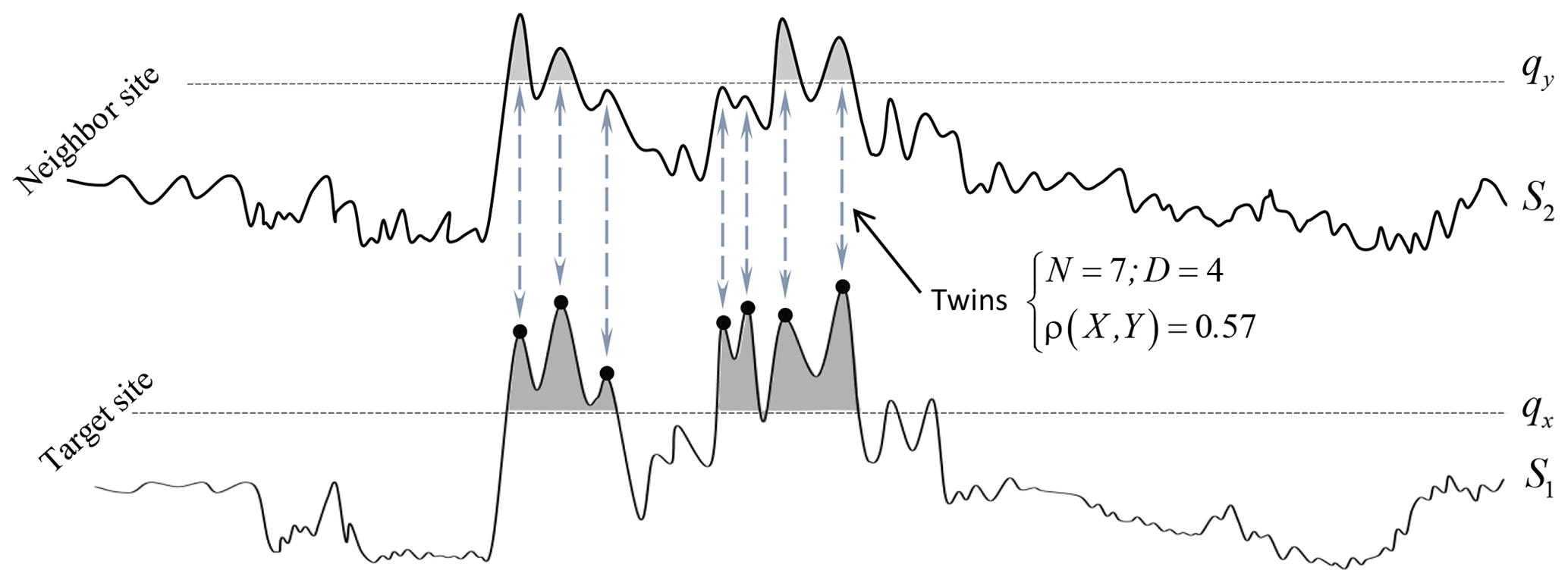
Figure 1An illustrative example on how the extremal dependence coefficient is empirically computed. Among the seven extreme twins (N=7), only four overlapped with the target-site extreme storm surges (D=4). The extremal coefficient is then equal to 0.57.

Download

The scheme for obtaining the extremal dependence between a target site and all the other sites has to be applied differently for each case study. The first question one can ask is the following: from which value of the extremal dependence coefficient can two sites begin to be considered neighbors? This leads to some other questions: when does the extremal correlation begin to be statistically significant? Or from which value of ρ₀ do we begin to have a positive association between two sites (when they experience a significant simultaneous rise in water during a storm)? Objective answers to these questions cannot in any case suggest an exact value or a statistic under or above which things are different, but there is an area in the space of the parameter or a range of values that can be explored and, depending on the sensitivity to this coefficient conclusions, can be drawn.

Let ρ₀ be the threshold above which the probability of extremal dependence between X and Y is high enough to consider S₁ and S₂ inside the same physically homogeneous region. First and foremost, there is a trade-off associated with the selection of this threshold: a large value of ρ₀ can result in a homogeneous region that is too small, but the opposite is likely to cause a residual probability (nothing other than a noise) which interferes with the construction of the region. The threshold ρ₀ can be estimated by analyzing the pairwise extremal dependence probability (between all sites and the target site). This procedure allows for the evaluation of the maximum-residual-noise order of magnitude. In addition, the determination of “an optimal” ρ₀ has to allow for the data merging of the neighboring sites of the target site (which have an extreme dependence on it) and put aside the “false” neighbors (sites having a residual extremal dependence probability with the target site considered to be a noise). The empirical quantiles q₁ and q₂ are set in order to extract, in X and Y series, only extreme events per year, which allows for the computation of the empirical spatial extremal coefficient from the biggest storms of each year. We know intuitively that the threshold ρ₀ may vary depending on the climate of the region and other physical and physiographic factors such as the bathymetry and the presence or lack of presence of a tidal estuary. Finally, the target-site neighborhood contains all sites which have a probability of extremal dependence greater than ρ₀. From a physical point of view, this means that when a storm affects a given target site, it will likely impact (not systematically) only sites enclosed in the region of interest and vice versa. The neighborhood of the target site can also be considered the region of influence around the target site as introduced by Burn (1990).

2.2 Independent storm extraction and construction of the regional frequency model

Once the homogeneous region of interest centered on the target site is obtained, the procedure begins by constructing a regional sample of independent storms. A storm is defined as a physical event that induces extreme SSSs (i.e., exceeds the extreme quantile q_p) in at least one site in the region of interest. To extract independent extreme SSSs, only the maximum value is kept.

The RFA uses the flood index principal, which stipulates that within a statistically homogeneous region, extreme events normalized with a local index are drawn from a common regional distribution. It is assumed that the distribution of these extreme normalized SSSs converges to a generalized Pareto distribution (GPD) and the number of exceedances converges to a Poisson distribution. The annual SSS quantile was used as a local index to normalize on-site samples. A further noteworthy statistical setting of the developed RFA is that it uses a relatively high threshold, allowing the selection of extreme storms corresponding to an annual rate λ of extreme SSSs equal to 1. To meet and satisfy the statistical homogeneity requirement of the region of interest, two L-moment-based tests introduced by Hosking and Wallis (1997) are used: (i) the heterogeneity indicator H, which is a measure of whether the dispersion between sites is similar to a value that would be expected in a statistically homogeneous region, and (ii) the discordancy criterion D_c to ensure that any site is not significantly different, in terms of L moments, from the other sites. Hosking and Wallis (1997) suggest that a site is discordant if D_c<3. In addition, a region is considered “acceptably homogeneous” if H<1, “possibly heterogeneous” if $\mathrm{1}\le H<\mathrm{2}$, and “definitely heterogeneous” if H≥2. These tests are performed for each region of interest. A site is generally eliminated from the inference if it is found to be discordant. To make the best possible use of the expertise (to be more conservative, for instance), the results are compared with and without the inclusion of discordant sites.

2.3 Regional effective duration of observations

In a regional context, the effective duration of observations D_eff of the regional sample depends on those of local samples d_i(i=1, … N), where N is the number of sites in the region of interest. Indeed, D_eff must be filtered of any intersite or any spatial dependencies and correlations. If on-site samples in a given region are completely independent, pooling data from these sites leads to a regional effective duration of observations equal to ∑d_i. This is obviously not the case herein. In those cases where the intersite dependence is perfect, D_eff can be formulated as the average of durations of observations d_i. Weiss et al. (2014) have developed a spatial function φ that reflects the intersite dependence in a region of interest. Weiss et al. (2014) have shown that $\mathit{\phi }={\mathit{\lambda }}_{\mathrm{r}}/\mathit{\lambda }$, where λ_r is the average annual number of storms in the region and λ is the average number of storms per year at each site. D_eff is expressed as a weighted sum in the following form:

where n_r is the number of regional SSSs. The function φ takes a value between 1 and N according to the level of dependence in the region.

• φ=1 if the region is perfectly regionally dependent. The effective duration of observations D_eff takes then the form of the average of durations: $D_{\mathrm{eff}}=\mathrm{1}/N\sum d_i$.

• φ=N if the region is regionally independent. This leads to $D_{\mathrm{eff}}=\sum d_i$.

2.4 Fitting the regional SSSs and at target-site frequency estimations

The regional frequency model used herein is based on the extreme value theory. As mentioned in Sect. 2.2, the peaks-over-threshold (POT) approach (e.g., Pickands, 1975), in which the excesses are analyzed with the GPD, is used in the RFA, using a threshold equal to 1 and taking into account the seasonality. Seasonal effects, considered for other variables in the literature (e.g., Morton et al., 1997; Méndez et al., 2008), can be modeled through a sinusoid. The regional distribution becomes a discrete mixture of GPD and sinusoid, with a seasonally varying scale parameter ξ (ξ varies periodically and smoothly across the seasons) (Weiss, 2014). The probability distributions are constructed as follows.

Let us denote v the regional random variable. A GPD is fitted to the regional sample, taking into account the four seasons in the following way:

p_r,c is the frequency of occurrence of season c in the regional sample (empirically estimated as the observed proportion of storms that occurred during season c in the region). We also have

and

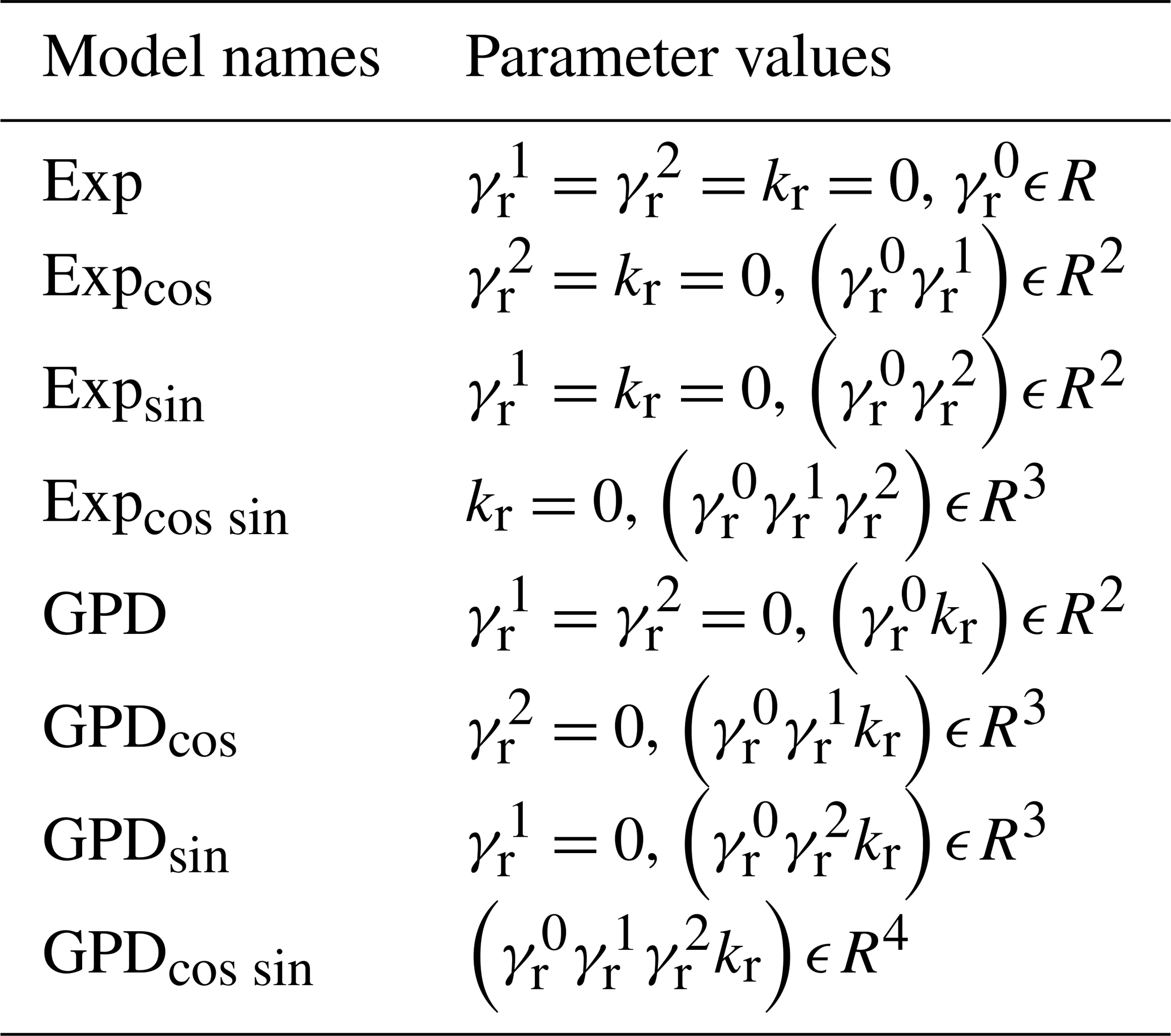
where ${\mathit{\gamma }}_{\mathrm{r}}^{\mathrm{0}}$, ${\mathit{\gamma }}_{\mathrm{r}}^{\mathrm{1}}$, and ${\mathit{\gamma }}_{\mathrm{r}}^{\mathrm{2}}$ are three parameters to be estimated. Table 3 presents the eight models derived from the possible values of ${\mathit{\gamma }}_{\mathrm{r}}^{\mathrm{0}}$, ${\mathit{\gamma }}_{\mathrm{r}}^{\mathrm{1}}$, ${\mathit{\gamma }}_{\mathrm{r}}^{\mathrm{2}}$, and k_r. Besides the visual inspection of the fitting curve, the Akaike information criterion (AIC) is used to select the more adequate distribution. Finally, the frequency estimation can be easily reverted to estimate the on-target-site SSRLs by multiplying the regional ones by the local index (i.e., the annual SSS quantile).

2.5 The case study

SSS datasets are obtained from the temporal series of hourly observations and predicted tide levels (the astronomical tide), collected at a total of 67 sites located on the Spanish, French (Atlantic and English Channel), and British coasts (see Fig. 2). The French tide gauges are managed by the French oceanographic service (SHOM – Service Hydrographique et Océanographique de la Marine), while Spanish and British ones are managed by IEO (Instituto Español de Oceanografía, Spain) and the British Oceanographic Data Centre (BODC), respectively.

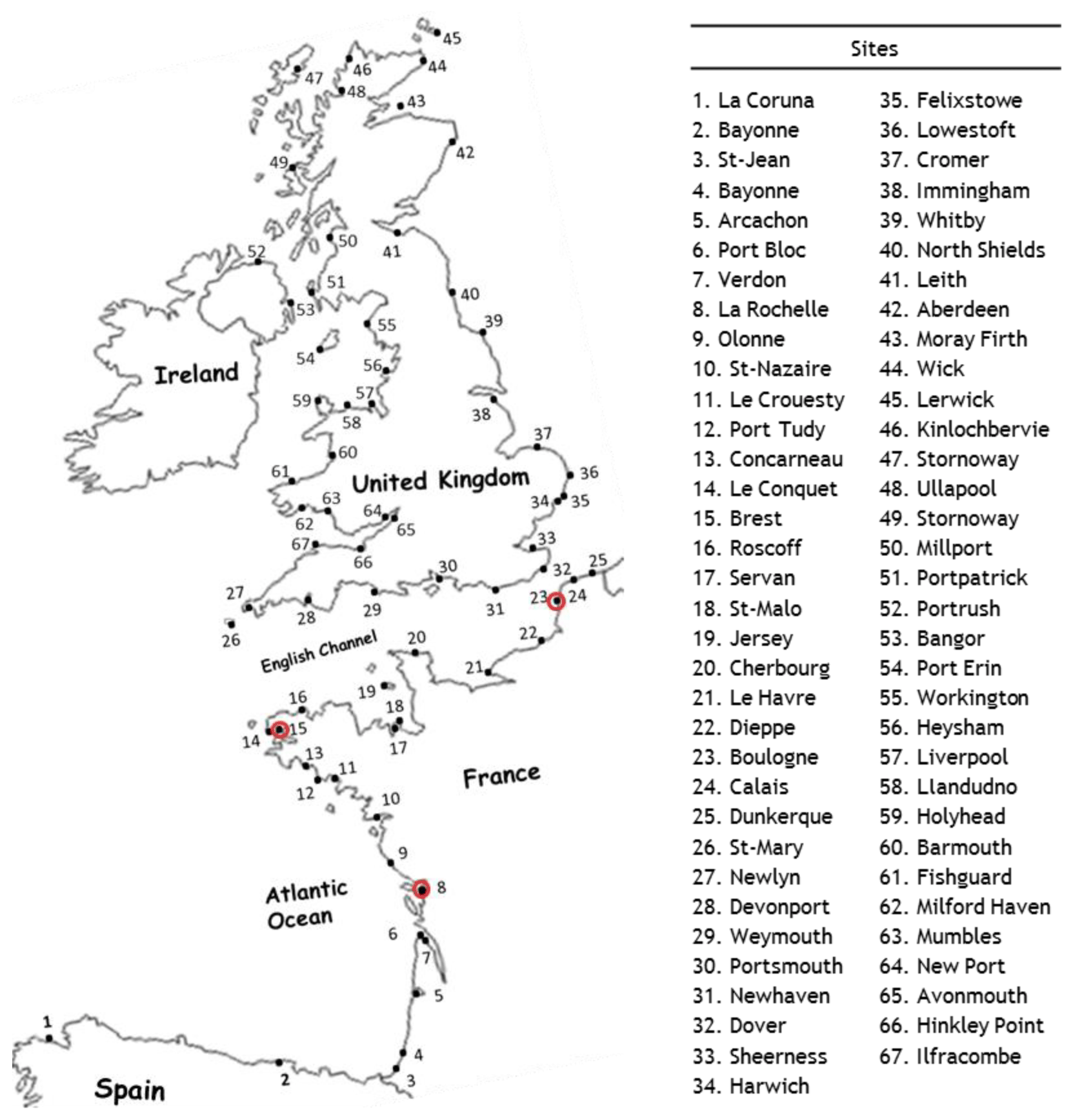
Figure 2Location of sites used for the study: 67 ports along the Spanish, French, and British coasts. Each site is associated with a number. The table on the right shows the correspondence between numbers and sites. The circled points represent the target sites for which a centered RFA is carried out in this study.

For convenience, the same observation periods as those used by Weiss (2014) were used in the present study. They range from 1846 for Brest (in France) to 2011 (for almost all the sites), and they show an average effective duration of observations of 31 years. In most cases, local series are characterized by the presence of many gaps. It is to be noted that the sea levels must be corrected from a possible eustatism (a general variation in mean sea level) in order to avoid inducing bias in the calculation of the surges: a correction is done if annual sea levels (calculated following the Permanent Service for Mean Sea Level recommendations) show significant trends. It is also noteworthy that the impact of climate change on the estimated return levels and associated uncertainties is not covered by this paper. The use of projected sea level rise could, however, be the subject of another paper.

Furthermore, in connection with the choice of the variable of interest, the focus is restricted to SSS series because in regions with strong tidal influence, the coastal flooding hazard is most noticeable around the time of high tide. Indeed, the SSS is a fundamental input for many statistical investigations of coastal hazards. It is defined as the difference between the maximum observed sea level and the one predicted around the time of high tide. Thus, the resulting SSS series have a temporal resolution of approximately 12.4 h. The reader is referred to Bernardara et al. (2011) for a more detailed introduction on skew surges. The developed RFA is performed at many target sites along the French (Atlantic and English Channel) coast. One of the most important features of these target sites is the fact that the region in which they are located has experienced significant storms during the last few decades (1953, 1987, Lothar and Martin in 1999, and Xynthia in 2010). Figure 2 displays the geographic location of the whole region. As depicted in the left-hand side of the figure, three target sites (red empty circles) are selected to perform the developed methodology and estimate the 1000-year return level.

3.1 Formation of regions of interest centered on target sites

Two types of thresholds are used in the calculation of the empirical spatial extremogram. The first threshold sets the extreme quantiles to extract extreme SSSs, and the second one (the neighborhood threshold) sets the extremal coefficient above which sites are considered neighbors. Since thresholds that are too high result in introducing a high variance and those that are too low introduce a bias in the results, there is a trade-off to be made between variance and bias. Indeed, the asymptotic properties of the marginal SSSs can be violated when too low of an extreme quantile q_p (p<70 %, for instance) is used to compute the extremal dependence coefficient of a given site. The use of too high of a threshold (p>99 %, for instance) can significantly reduce the number of the pairs of simultaneous extreme events to be used to compute the extremal coefficient. It is to be noted that, even if the q_p threshold is adequately selected, too high of a neighborhood threshold (ρ₀>0.7, for instance) will limit the number of neighboring sites and decrease the size of the region of interest, while too low of a threshold will likely cause a residual probability (which is nothing other than a noise) and will erroneously increase this region. Values of q_X and q_Y are tested in order to select four and then six storms a year, which finally give information from the empirical spatial extremogram that leads to similar regions. Therefore, the extremal quantiles are set to select only four storms a year. This value allows for the computation of the empirical spatial extremogram from the biggest storm of each year. Moreover, the lag time h has to be large enough to allow a storm which occurs at one site to propagate eventually to the other site. Spatial extremograms performed with lag times greater than 24 h show little difference compared to those obtained with lag times equal to zero and to the duration between two SSSs (about ±12.4 h). The latest two lag times are then used, and the greatest value among the corresponding extremal coefficients is kept. Finally, the neighborhood threshold is set to 0.3. This value allows for the elimination of any sites associated with a value of the spatial extremal coefficient that look like a residual noise.

3.1.1 Calais (station number 24)

One of the most important features of the Calais site is the fact that it is located close to a border of one of the regions found by Weiss (2014). In addition, the region in which this site is located has experienced significant storms during the last 2 decades (Martin in 1999 and Xynthia in 2010). Figure 3 displays the geographic location of five homogeneous regions according to Weiss (2014). The scheme for obtaining the pairwise extremal dependence coefficients between Calais as a target site and all the other sites is applied herein. From the ESE depicted in the Fig. 4a, a geographically coherent region of interest corresponding to the neighborhood threshold (ρ₀=0.3) is obtained and illustrated in the leftmost panel of Fig. 5. As can be seen in Fig. 4, the pairwise probabilities of the extremal dependence between Calais and all the sites in the whole region are presented on the vertical axis. The sites of the whole region, presented on the x axis, are sorted in an ascending order based on the geographical distance to the target site. The physically homogeneous group of sites with extremal dependence probabilities greater than ρ₀ (the red lines on Fig. 4) are considered to be potential neighbors of the target site (Calais) and are thus part of the region of interest (of Calais). The pairwise simultaneous length of record (at the target site and any site of the whole region) appears in brackets next to the name of each site in Fig. 4. This duration is an important setting because it is the number of years on which the spatial extremal coefficients are calculated. For instance, the time during which Calais and Dunkerque (station number 25) operated simultaneously is equal to 26 years. It is noteworthy that the probability of the extremal dependence may not be relevant if this time period is too small, and whether it is appropriate to consider the site in the inference will be assessed on a case-by-case basis. As shown in the leftmost panel of Fig. 5, the target site Calais is no longer located at the border of the region. Indeed, the physically homogeneous region of interest around Calais is slightly smaller than the one obtained by Weiss (2014) but more centered on Calais. Further noteworthy features of the ESE are that it provides regions smaller than those obtained by Weiss (2014) and that are more physically homogeneous.

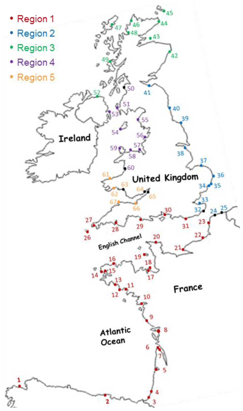
Figure 3Five physically and statistically homogenous regions (according to Weiss, 2014). The regions are represented by five colors. This figure shows that, for example, site 24 (Calais) is located in the region shown in blue and is very close to a border. Site 23 (Boulogne), however, which is very close to site 24 (Calais), is nevertheless in another region (the region shown in red). This separation between site 23 and site 24 may seem artificial.

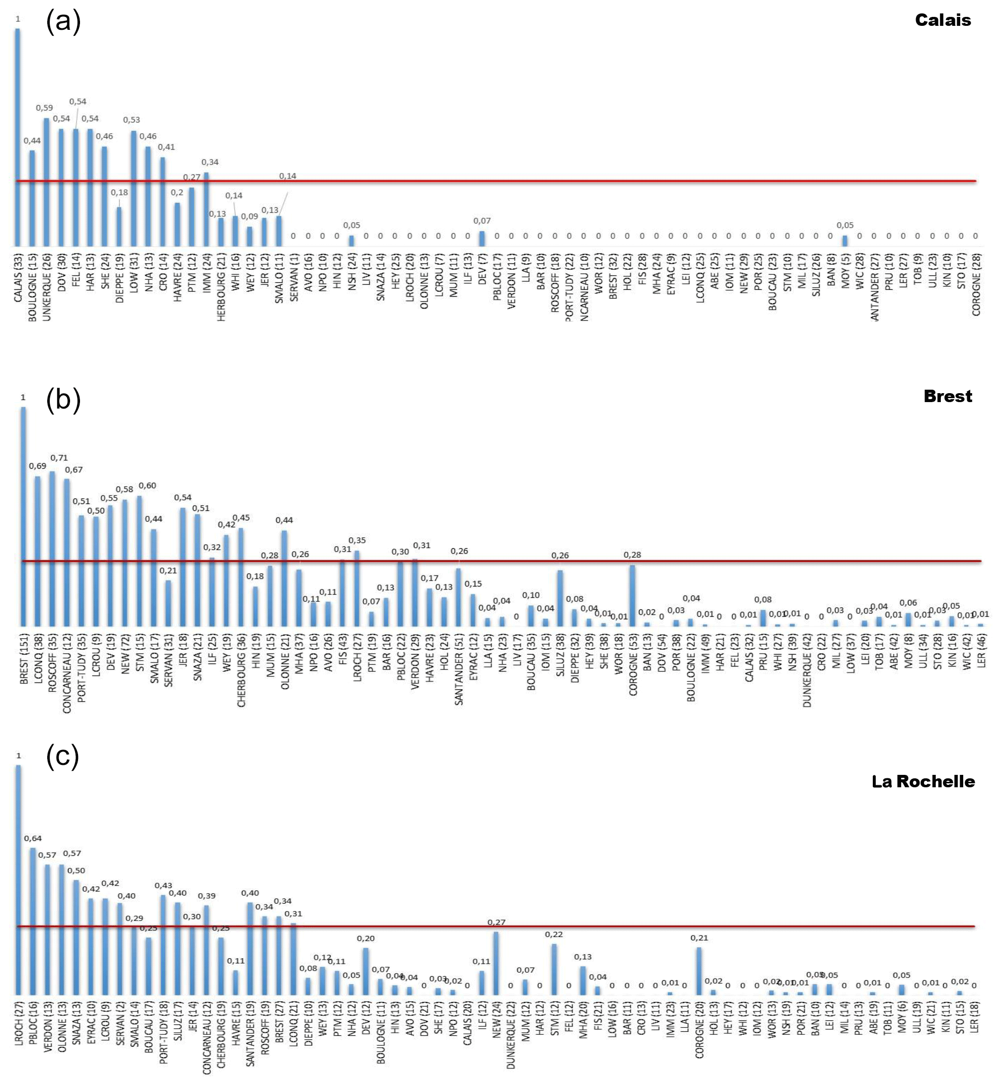
Figure 4The ESE for Calais (a), Brest (b), and La Rochelle (c). The abbreviations of the horizontal axis are presented in Fig. 2. The vertical blue bars have lengths proportional to the extremogram values. The value of each extremogram is indicated above the blue bars. The red line represents the threshold (equal to 0.3) above which the extremogram value is large enough that the associated site can be considered to belong to the same region as the target site. The overlap period (in years) of the observation periods of each site with that of the target site is indicated in the brackets next to each site name.

Download

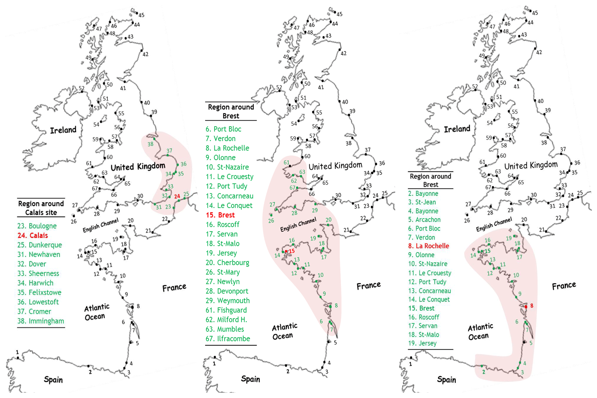
Figure 5Physically homogenous regions (the list of sites belonging to a region are surrounded by red zones) for Calais, Brest, and La Rochelle. Neighboring sites are represented with green dots (target sites are represented with red dots). Target sites are not close to a border.

3.2 The regional and local frequency estimations

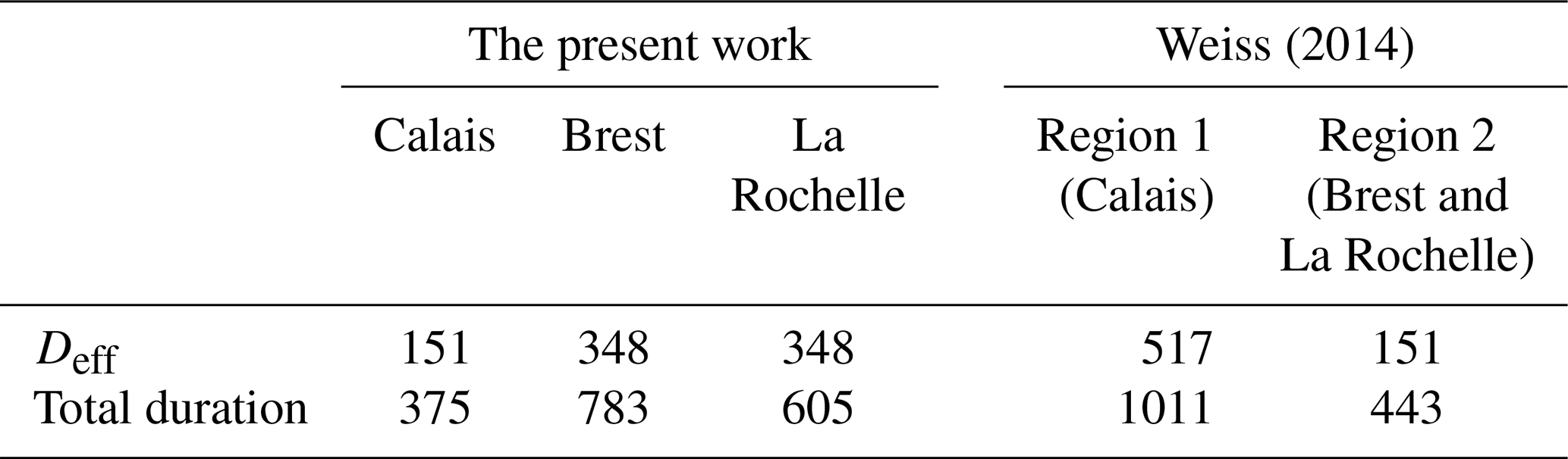
As mentioned earlier in this paper, a regional pooling method to estimate the regional distribution for each homogeneous region is used. Indeed, a storm that can impact several sites (thus generating intersite dependence) during a single storm is considered only once in the regional sample. The distribution of the maximum regional SSSs (M_s) is assumed to be identical to the regional distribution. In order to verify the validity of this assumption, a Kolmogorov–Smirnov test (H_o: the regional observations and M_s sample follow the same distribution) is performed. The null hypothesis H_o is satisfied for the three regions centered on Calais, Brest, and La Rochelle at a risk level of 5 %. Consequently, the regional distribution can be estimated from each regional sample M_s. The way the delineation of the homogeneous regions is performed implies that the regional sample is characterized by a strong spatial dependence which impacts, in a first step, the regional effective duration of observations D_eff (that will be even lower if this dependence is high). The effective duration of observations D_eff is calculated using Eq. (3), and the results are compared with those obtained by Weiss (2014). These results are summarized in Table 1. It is important to remember here that in the study of Weiss (2014), Calais is a part of region 2, while Brest and La Rochelle are located in region 1. As shown in Table 1, the regional effective duration of observations D_eff associated with the region of Calais is the same in both studies. However, it is smaller in the present work for the region of Brest and La Rochelle. In any case, however, regional effective durations are obviously higher than local ones. Furthermore, a Student t test is performed to check if the regional sample is stationary in intensity (two subsamples have equal means) or not. It is concluded that all the samples are stationary in intensity.

Table 1Comparison of total and effective durations of observations (years) used in the present study with those used by Weiss (2014). The effective duration of observations takes into account the intersite dependence. A total duration of observations is the sum of all on-site durations in the region of interest (without intersite dependence).

Download Print Version | Download XLSX

A GPD distribution taking into account the seasonality is then fitted to the regional sample. The distribution parameters are estimated with the penalized maximum likelihood method (Coles and Dixon, 1999). The most adequate distributions are obtained with the AIC. The Exp_sin distribution is selected for Calais, while it is concluded that the distributions of the extreme regional SSSs for Brest and La Rochelle converge to a Gpd_cos  sin. The same frequency models are selected by Weiss (2014) for regions 2 (including Calais) and 1 (including Brest and La Rochelle), respectively. The reader is referred to Weiss (2014) to learn more about the mixture of GPD–sinusoid distributions with a seasonally varying scale parameter. The fitting curves for Calais, Brest, and La Rochelle, which are shown in Fig. 6, look good. Indeed, most of the points in the body of the distribution are inside the confidence intervals. Those elements are also relevant for accepting the credibility of the distributions used for the fitting.

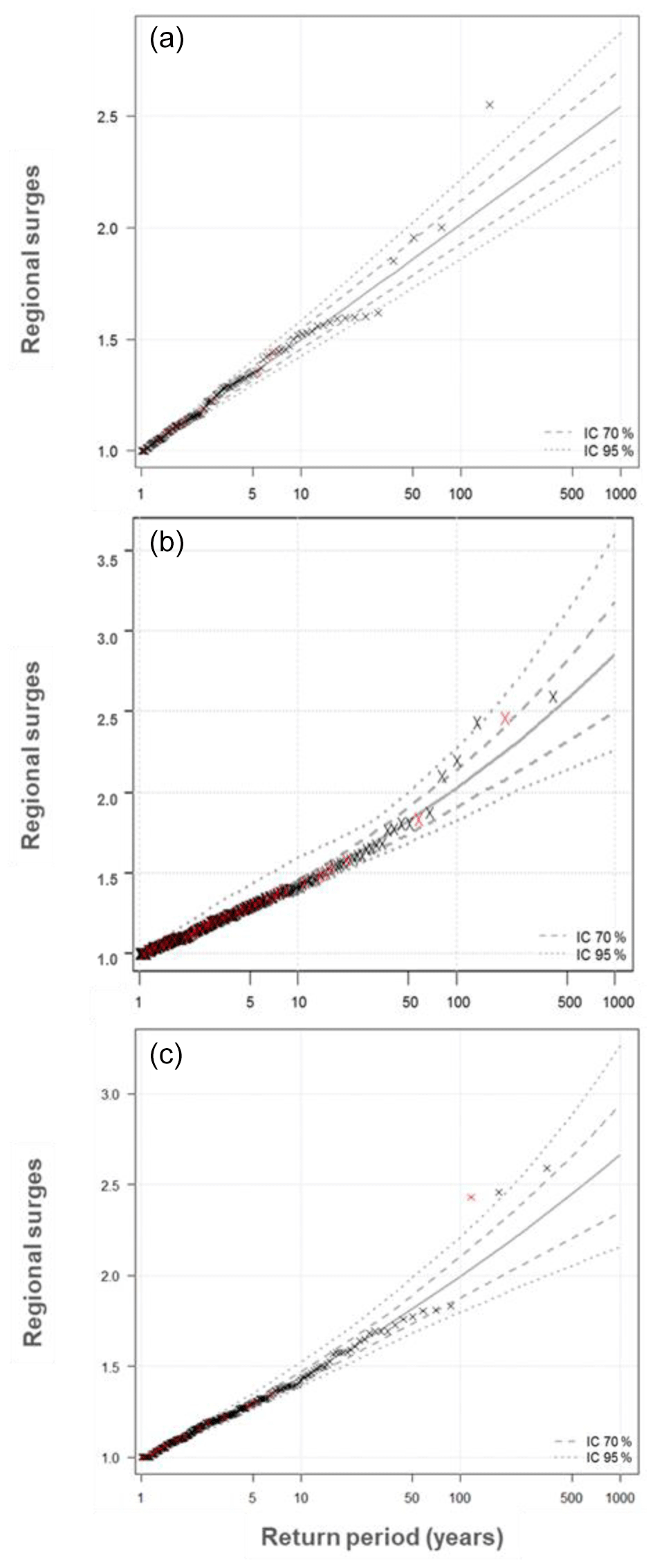
Figure 6The GPD–sinusoid fitted to regional SSSs (plotting positions, RLs, and confidence intervals) for the target sites: Exp_sin distribution for Calais (a) and GPD_cos  sin for Brest (b) and La Rochelle (c). The y axis represents the normalized regional surges (without unit); the x axis represents the return period (in years). The red crosses indicate the SSSs at the target site, so the black crosses indicate the regional ones. The confidence intervals at 70 % (dashed line) and 95 % (dotted line), which are computed by the bootstrap method, are also presented (dotted lines).

Download

In the next RFA step, local quantiles are estimated by multiplying the regional ones by the local indices. The results are summarized in Table 2, presenting a comparison of the 1000-year return levels with associated confidence intervals.

Table 2Comparison of the 1000-year return levels with the 70 % of the confidence interval width (70 % CI) in brackets obtained herein with those of Weiss (2014).

Download Print Version | Download XLSX

Table 3Possible models for the fitting of the regional samples.

Download Print Version | Download XLSX

It is worth concluding that better centering the region of interest on the Calais site did not significantly change quantiles (a decrease of only 7 cm) but rather narrowed the associated confidence interval of about 12 cm. This outcome refers only to the region of interest around Calais, and it is different for the region centered on Brest and La Rochelle sites. However, the quantiles and associated confidence intervals are overall roughly the same, but the method presented herein better answers the uncertainties linked to the border effect issue, notably through the ESE tool.