the Creative Commons Attribution 4.0 License.
the Creative Commons Attribution 4.0 License.
 | 07 Jan 2020
Simulations of the 2005, 1910, and 1876 Vb cyclones over the Alps – sensitivity to model physics and cyclonic moisture flux
Peter Stucki
Paul Froidevaux
Marcelo Zamuriano
Francesco Alessandro Isotta
Martina Messmer
Andrey Martynov
In June 1876, June 1910, and August 2005, northern Switzerland was severely impacted by heavy precipitation and extreme floods. Although occurring in different centuries, all three events featured very similar precipitation patterns and an extratropical storm following a cyclonic, so-called Vb (five b of the van Bebber trajectories) trajectory around the Alps. Going back in time from the recent to the historical cases, we explore the potential of dynamical downscaling of a global reanalysis product from a grid size of 220 to 3 km. We investigate sensitivities of the simulated precipitation amounts to a set of differing configurations in the regional weather model. The best-performing model configuration in the evaluation, featuring a 1 d initialization period, is then applied to assess the sensitivity of simulated precipitation totals to cyclonic moisture flux along the downscaling steps. The analyses show that cyclone fields (closed pressure contours) and tracks (minimum pressure trajectories) are well defined in the reanalysis ensemble for the 2005 and 1910 cases, while deviations from the ensemble mean increase for the 1876 case. In the downscaled ensemble, the accuracy of simulated precipitation totals is closely linked to the exact trajectory and stalling position of the cyclone, with slight shifts producing erroneous precipitation, e.g., due to a break-up of the vortex if simulated too close to the Alpine topography. Simulated precipitation totals only reach the observed ones if the simulation includes continuous moisture fluxes of >200 kg m−1 s−1 from northerly directions and high contributions of (embedded) convection. Misplacement of the vortex and concurrent uncertainties in simulating convection, in particular for the 1876 case, point to limitations of downscaling from coarse input for such complex weather situations and for the more distant past. On the upside, single (contrasting) members of the historical cases are well capable of illustrating variants of Vb cyclone dynamics and features along the downscaling steps.
Please read the corrigendum first before continuing.
-
Notice on corrigendum
The requested paper has a corresponding corrigendum published. Please read the corrigendum first before downloading the article.
-
Article
(22998 KB)
-
The requested paper has a corresponding corrigendum published. Please read the corrigendum first before downloading the article.
- Article
(22998 KB) - Corrigendum
- BibTeX
- EndNote


Floods are among the most damaging natural hazards worldwide (SwissRe, 2018); they affect more people than any other natural hazard (McClean and Guha-Sapir, 2019). The costliest flood event in Switzerland of the last decades occurred in 2005 (Hilker et al., 2009); it caused fatalities and led to heavily damaged infrastructure (Bezzola et al., 2008). This event was well documented and subsequently a range of publications analyzed the flood-inducing meteorological conditions (e.g., Frei, 2005; Beniston, 2006; MeteoSwiss, 2006; Bezzola and Hegg, 2007, 2008; Zängl, 2007a; Hohenegger et al., 2008; Jaun et al., 2008; Langhans et al., 2011; Stucki et al., 2012; Messmer et al., 2017).
On a synoptic scale, the associated extratropical cyclone mainly followed the classical so-called Vb (five b of the van Bebber trajectories) cyclone track after Köppen (1881) and van Bebber (1891); see also Hofstätter et al. (2016). Cyclones on a Vb track are associated with heavy to extreme precipitation over central Europe, particularly north of the Alps (Hofstätter et al., 2016, 2018; Nissen et al., 2014). Most of the cyclones following the Vb trajectory are generated in the western Mediterranean region, and most of them pass the Gulf of Genoa region (Hofstätter and Blöschl, 2019; Messmer et al., 2015). For this reason, they are also called “Genoa lows” at this stage (Bezzola et al., 2008). They take up moisture over the Ligurian Sea then propagate eastward to the Adriatic Sea and curve northward again (Hofstätter et al., 2018; Hofstätter and Blöschl, 2019; Messmer et al., 2015; Pfahl, 2014; Ulbrich et al., 2003). Regarding the pattern of mid-tropospheric geopotential heights, the 2005 case has also been characterized as a pivoting cutoff low (PCO; Stucki et al., 2012; Froidevaux and Martius, 2016), referring to the recurving track of the system around the Alps while its axis of symmetry turns from meridional to zonal; see also Awan and Formayer (2017) for a general description of cutoff lows and their influence on extreme precipitation in the European Alps. Furthermore, quasi-stationarity (i.e., stalling) of the system over northern Italy was important: in the cyclonic circulation around the Vb cyclone, large quantities of warm and humid Mediterranean air were transported over and around the eastern Alps. This dynamic mechanism is described as “cyclonic moisture flux” hereafter. With the term cyclonic, we refer to the pattern of moisture flux streamlines, forming a (closed) counterclockwise rotation around the cyclone center. Downstream, the cyclonic moisture flux impinged onto the slopes of northeastern Switzerland from the northern sector (Hohenegger et al., 2008; Froidevaux and Martius, 2016; Messmer et al., 2017). The intensity of the integrated water vapor transport (IVT) was estimated to exceed 300 kg m−1 s−1 (Froidevaux and Martius, 2016). Hence, IVT was found to be an important precursor for severe floods in Switzerland (cf. Kelemen et al., 2016, for a European summer flood in 2013). Precipitation occurred in two peak episodes in the afternoons of 21 and 22 August 2005, when stratiform upslope orographic precipitation was locally enhanced by embedded convection (Hohenegger et al., 2008; Langhans et al., 2011).
Although the impact of the 2005 event was very severe, it was not unique in a historical context. Several studies found similar spatial distributions of damage and precipitation, as well as similar synoptic-scale weather patterns. Two such analog cases occurred in June 1910 and June 1876 (Röthlisberger, 1991; Pfister, 1999; Frei, 2005; Stucki et al., 2012). For instance, their similarities were analyzed on a synoptic scale using the Twentieth Century Reanalysis (20CR; Compo et al., 2011) and classified as PCO type 1 (2005, 1910) and type 2 (1876), where the 1876 case features a more northwesterly flow towards the Swiss Alps (Stucki et al., 2012).
However, two options for hydrometeorological analyses have not been considered so far to learn from these historical cases. The first option is the systematic use of a reanalysis ensemble to assess sensitivities of the severe weather in regards to determining factors such as cyclone trajectories or IVT. The second option is using global reanalysis products for dynamical downscaling to mesoscale resolutions, i.e., the nesting of limited-area weather models into larger-scale models in several refinement steps (von Storch et al., 2000; von Storch and Zorita, 2019). In fact, 20CR has proven to be a valuable input dataset for downscaling heavy-precipitation and windstorm events over the Central Alps back to the 19th century. Stucki et al. (2018) showed that downscaling the ensemble mean is not only computationally cheaper but also can be seen as a minimum-error approach and thus natural approach in well-represented areas and distinctive synoptic flow conditions. For an extreme flood in 1868, they found a small smoothing effect of the associated cyclone, which induced southerly moisture flux, i.e., perpendicular to the Alpine range. In contrast, the present study includes more complex and transient Vb flow situations. For such cases, using the full ensemble is recommended for deriving an uncertainty estimation (e.g., Welker and Martius, 2015). For instance, Hohenegger et al. (2008) assessed the benefits of a limited-area ensemble prediction system for forecasting precipitation.
For dynamical downscaling, there are manifold options regarding the configuration of the limited-area weather models, including the choice of adequate reanalysis products as input datasets, initialization spans (so-called spin-up), spatial extent and resolution of the simulation domains, or model physics (e.g., Prein et al., 2015). To date, only 20CR covers the 1876 case, at the expense of a coarse grid size of 2∘ × 2∘ in the horizontal, while finer-resolved reanalysis products have been used to downscale cases after 1900 (e.g., Brugnara et al., 2017). Regarding the initialization, long spin-ups would allow soil moisture and similarly slow-adapting model variables to reach an equilibrium, although the information from the initial conditions is lost with advancing time in the simulation. In turn, short spin-up times constrain the potential evolution close to the large-scale input. For Vb cyclones, relatively short spin-ups were chosen by Hohenegger et al. (2008) and Messmer et al. (2015, 2017). Regarding spatial resolution, cloud-resolving and convection-permitting grid sizes equal to or lower than about 3 km are necessary to reproduce the precipitation of the 2005 case (Zängl, 2007b; cf. Prein et al., 2015). Typical setups of limited-area models mostly include explicit production of precipitation in the innermost domain, while convection is parameterized for the coarser domains. Further options are one- versus two-way nesting or nudging in one or more domains.
In this study, we assess the 2005, 1910, and 1876 cases in two ways. First, we aim to find a setup of the Weather Research and Forecasting (WRF) model (Skamarock et al., 2008) that is adequate for dynamical downscaling from 20CR and for our cases. For this, we use the 2005 case as test bed because of the large amount of observations available for verification. Second, we apply the chosen setup to all three cases, aiming to investigate relevant atmospheric features that induce heavy precipitation and to assess the inevitably increasing uncertainty along the downscaling steps and among the ensemble members as we go back in time from 2005 via 1910 to 1876.
The article is organized as follows. Data and models are introduced in Sect. 2. The evaluation of different model setups is described in Sect. 3. The synoptic and mesoscale reconstructions of the three cases are presented in Sect. 4. A summary and conclusive remarks are given in Sect. 5.
2.1 Observation-based precipitation datasets
All observation-based precipitation datasets used in this study come from the Federal Office for Meteorology and Climatology, MeteoSwiss. Precipitation totals derived from all three observation-based products are shown in Fig. A1. The first dataset is observations of daily precipitation totals. These measurements are quality checked and homogenized according to Füllemann et al. (2011).
CombiPrecip, the second product, is also a gridded dataset. It results from a geostatistical combination of rain-gauge observations and radar images. It covers the entire Swiss territory for the period 2005 to present at high spatial and temporal resolutions. The hourly precipitation accumulation is available as a running sum updated every 10 min on a 1 km grid.
The third MeteoSwiss product is RrecabsD, a prototype dataset specifically calculated for this study with a statistical reconstruction technique. The procedure was previously used to reconstruct monthly and daily precipitation in the Alps for different scopes (Isotta et al., 2019; Masson and Frei, 2016; Schiemann et al., 2010; Schmidli et al., 2002). It involves a principal component analysis (PCA) of a high-resolution grid dataset in a calibration period defined between 1981 and 2010 and an optimal interpolation of PCA scores from long-term station data. The high-resolution dataset used for the PCA is RhiresD (MeteoSwiss, 2006) on a grid size of 2.2 km, with daily precipitation totals retrieved by spatial interpolation of rain-gauge measurements within the Swiss borders. In RrecabsD, the focus is on spatial consistency by using all station measurements available both in the respective days in 1910 or 1876 and in a consistent part of the calibration period (1981–2010), which is accordingly slightly reduced by eliminating the days with gaps at one or more of the chosen stations. The three datasets described above integrate observational information and are used as reference. They are, like other dataset, affected by uncertainties and errors, which were analyzed in detail in the provided references and in several applications.
2.2 Reanalysis datasets
The Twentieth Century Reanalysis dataset version 2c (20CR; Compo et al., 2011) is used for synoptic analyses and as initial and boundary conditions for the downscaling experiments. 20CR is a global atmospheric reanalysis with a 2∘ spatial grid (approx. 220 km over Europe), 28 vertical hybrid-sigma pressure levels and 6-hourly temporal resolution going back to 1851. Only surface pressure observations are assimilated. Over the time period of the 1876 case, four stations within Switzerland are used in the assimilation (Bern, Sion, Grand St. Bernard, and Geneva). This number grows to six for the 1910 case (including also Zurich and Basel), and to 34 for the 2005 case. The 20CR ensemble mean and 56 members are available.
The ERA-Interim (Dee et al., 2011) and CERA-20C reanalyses (Laloyaux et al., 2016) are used for comparisons of synoptic fields to 20CR. ERA-Interim (CERA-20C) has a horizontal grid size of approx. 80 km (125 km), 37 (37) pressure levels, 6 h (3 h) temporal steps, and reaches back to 1979 (1901). ERA-Interim is also used as initial and boundary conditions for downscaling the 2005 case to compare with downscaling based on 20CR.
2.3 Regional model WRF
The nonhydrostatic Weather Research and Forecasting model (WRF-ARW Version 3.7.1; Skamarock et al., 2008) is used for dynamical downscaling of the 2005, 1910, and 1876 cases. Here, we describe the final model configuration, which was determined by an evaluation of different tuning options (see Sect. 3).
In the selected configuration of the WRF model, initialization is set to 20 August 2005 06:00 UTC, while the largest precipitation totals were observed on 22 August 2005. This allows for model initialization over a period of approximately 24 h. The horizontal setup consists of four nested domains with grid sizes of 81, 27, 9, and 3 km. The innermost domain covers much of the Alpine bow to avoid complex terrain at the boundaries (Fig. 1). The vertical setup consists of 60 eta levels (with a top level of 50 hPa) to capture fine-scale features of vertical lifting and condensation. The Thompson microphysics scheme (Thompson et al., 2008) is used for bulk microphysical parameterization after a first check against the Morrison scheme (Morrison et al., 2009; not shown). Additionally, we use the Yonsei University (YSU) planetary boundary layer (PBL) scheme (Hong et al., 2006) for parameterizing turbulent fluxes with a correction for complex orography effects to the finest domain (Jiménez and Dudhia, 2012). The Kain–Fritsch cumulus parameterization is used in the larger domains (Kain, 2004) and turned off in the innermost domain. Moderate spectral nudging (corresponding to a wavelength of about 1500 km) is applied to temperature, wind, and geopotential fields above the PBL in the outermost domain to ensure consistency with the large scale forcing (von Storch et al., 2000). The downscaling output is stored in hourly resolution.
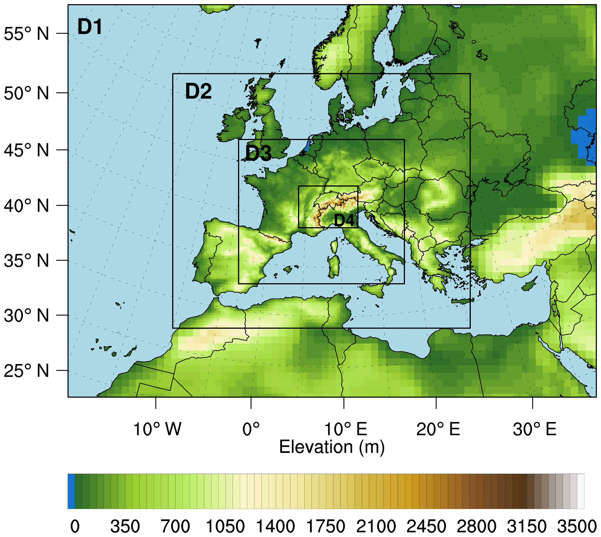
Figure 1Nesting of the WRF regional model into 20CR, where D1 to D4 refer to the simulation domains with 81, 27, 9, and 3 km grid sizes. Shading indicates model topography for each domain in meters above sea level (m a.s.l.)
3.1 Setup of downscaling experiments
The WRF model configuration described above has been selected from a range of 10 setups. They differ in two perspectives. The first perspective involves increasing the initialization period from 1 to 3, 5, 7, and 10 d (see also Tables 1 and 2 for details) to check for potential enhancements of the simulations. With a 1 d spin-up, both early and late onsets of the most intense precipitation in different regions of the Central Alps are still captured. The 10 d initialization experiment is based on the assumption that an ample spin-up time of more than a week is desirable for the inner domains to reach some internal equilibrium. For example, the accumulation of soil moisture can significantly contribute to enhanced convection and precipitation, and it should therefore be considered (Zbinden, 2005; MeteoSwiss, 2006; Bezzola and Hegg, 2007; Cioni and Hohenegger, 2017).
Table 1Abbreviations and description of setup experiments*.
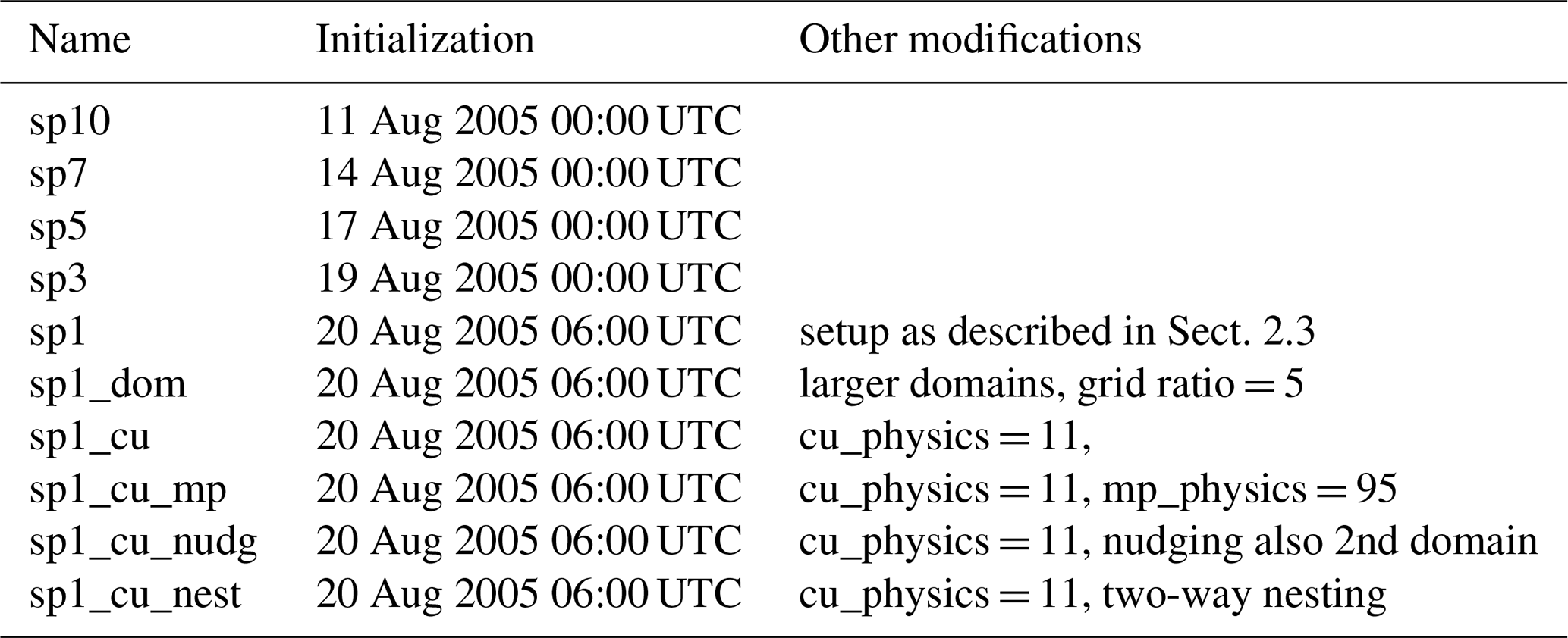
* Changes are indicated with respect to the setup with a 1 d spin-up period (sp1): the abbreviation sp5 indicates a change in the spin-up period to 5 d, mp indicates a change of the microphysics scheme, cu a different cumulus scheme, nudg indicates nudging in two domains, nest indicates two-way nesting, and dom stands for a larger domain. See text for details.
Table 2Evaluation of WRF setups for dynamical downscaling*.
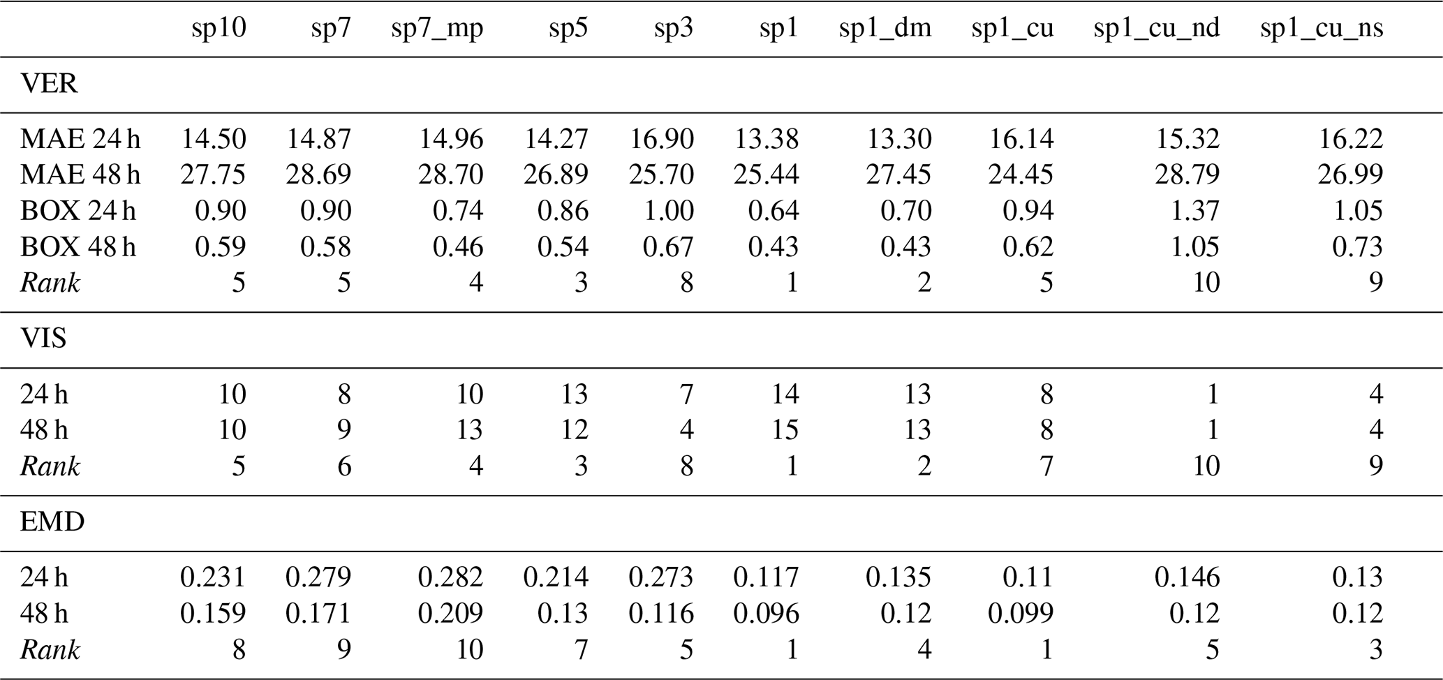
* Spatial verification measures for evaluating the performance of 10 different WRF simulation setups (columns; see Table 1 for abbreviations) against observations (CombiPrecip fields) of 24 and 48 h precipitation totals in a rectangle box over northeastern Switzerland (see Fig. A1), each calculated over a subset of 10 ensemble members. The top section shows two verification (VER) measures, i.e., (i) mean absolute error (MAE) of simulated versus observed precipitation totals (millimeter per 24 h or millimeter per 48 h), and (ii) mean absolute deviation of the simulated box ratios from the observation-based box ratio (specific rows denoted with BOX). For instance, the value of 0.9 (0.49) for sp10 and 24 h (48 h) precipitation totals indicates the mean absolute deviation from the observation-based value of 1.99 (2.26) in CombiPrecip. The middle section shows the scores from visual inspection (VIS), and the bottom section considers the spatial distribution of precipitation inside the box (EMD; see text for details). Ranks are added to all sections; ties are set equal.
The second perspective involves modifying a number of tuning options of the WRF model which may have an influence on the simulation performance according to literature and from our experience. The goal of these experiments is not to achieve a thorough sensitivity assessment for each tuning option but to make sure that we have not chosen a suboptimal setup. Concretely, we test larger domains since the high-resolution domain does not cover the entire extent of the cyclone. For this test, we also increase the grid ratio from three to five. Another test involves changing the cumulus scheme from Kain–Fritsch to Multi-scale Kain–Fritsch (Kain, 2004). Multi-scale Kain–Fritsch contains a grid resolution dependence, which may improve the location and intensity of precipitation in high-resolution simulations (Zheng et al., 2016). Furthermore, the microphysics scheme is changed from Thompson et al. (2008) to Ferrier (1994). The latter has been associated with higher precipitation totals over the USA (Schwartz et al., 2010). Among other differences concerning hydrometeors, ice, graupel and hail are represented in less detail. Note that the Morrison scheme (Morrison et al., 2009) had been discarded after a check with the original setup (Sect. 2.3). Moreover, nudging in the two outermost domains is applied to test for the effect of keeping the simulation close to initial conditions. Finally, one-way is compared to two-way nesting, also allowing for exchange of information from finer to coarser domains (cf. Bowden et al., 2012).
The evaluation of the downscaling experiments is done for the 2005 event, as only for this case simulations can be verified using a state-of-the-art spatial reconstruction of precipitation totals, which is CombiPrecip in our case. Recall that CombiPrecip also includes radar information. Both CombiPrecip and the WRF simulation are bilinearly interpolated to a 6 km horizontal grid for comparability and to reduce single-cell effects. For the verification, we focus on a control area in northeastern Switzerland (see the small box in Fig. A1), the region where most of the precipitation fell, and on precipitation totals over 48 h starting from 21 August 2005 06:00 UTC, i.e., the 2 d period with highest precipitation intensities (MeteoSwiss, 2006). In fact, precipitation was concentrated over northeastern Switzerland in the 2005 case, with gradients from the Alpine crests towards the Swiss Plateau. This spatial distribution was also important for the subsequent flooding (Bezzola and Hegg, 2007).
To save computational costs, the experiments are done with a subset of 10 members that cover the full range of precipitation variability from a first-guess setup (not shown). This original setup (in fact, the full ensemble of the 10 d initialization setup) resulted in a general underestimation of the accumulated precipitation in the control area compared to CombiPrecip, the reference dataset (Fig. A2).
3.2 Evaluation with respect to precipitation totals
We use three evaluation methods to determine an overall best-performing model setup for downscaling our cases.
The first evaluation is based on two spatial verification measures, i.e., mean absolute error (MAE) of the simulated versus CombiPrecip precipitation inside the control area and a metric using box ratios (see section VER in Table 2). The MAE measures the average distance between forecast and observation and is preferred over root-mean-square error (RMSE) because it is more resistant to outliers; it is also preferred over correlation coefficients because we are more interested in accuracy than linear association (Joliffe and Stephenson, 2012). Box ratio means the ratio of mean precipitation in the control area, i.e., the small box with respect to a larger box that encompasses Switzerland (see Fig. A1). The box ratio indicates how much of the precipitation is simulated in the correct region when compared to CombiPrecip. The box ratio in CombiPrecip for the 1 d (2 d) mean precipitation is 1.99 (2.26). In simple words, the mean observed rainfall was about twice as intense in the control area over northeastern Switzerland compared to all of Switzerland. For the evaluation, we calculate the mean absolute deviation of the simulated box ratios from the box ratio in CombiPrecip.
The second evaluation is based on visual inspection of the simulated precipitation totals, with a focus on the highest amounts of precipitation, i.e., the 4th quartile. Again, the according precipitation totals in CombiPrecip are used as a reference. The intersubjective judgment by the authors yields two points per downscaled ensemble member for a “good” match, one point for a “fair” match, and zero points for “mismatch” (see section VIS in Table 2). A good match is achieved in the case when the simulation places the highest quartile of precipitation in the correct regions when compared to the spatial patterns in CombiPrecip.
To contrast the subjective judgments, the third evaluation uses the earth mover's distance (EMD; Rubner et al., 1998, 2000) as a purely objective metric of similarity. The EMD, sometimes known as the Wasserstein distance, is typically used for pattern recognition in digital image processing and has as well been applied in atmospheric sciences, e.g., to pollutant concentrations, top-of-atmosphere radiation fluxes, time series of wind maxima, or precipitation and climate indices (Düsterhus and Hense, 2012; Baker et al., 2013; Farchi et al., 2016; Düsterhus and Wahl, 2018). Intuitively, it measures the cost (mass times distance) of turning one pile of dirt in one area into a second, reference pile, with the same overall mass and covering the same area. For our case, this means that the precipitation fields are normalized and hence the EMD considers only the relative patterns of precipitation. Specifically, the EMD indicates how well the simulated spatial distribution of the precipitation matches the observed distribution on a 6 km grid inside the control area. EMD is chosen over typical feature-based methods (e.g., the SAL method by Wernli et al., 2008) because it yields one number, involves less subjective choices and thresholds, and emphasizes the relative pattern. Section EMD in Table 2 gives the median distance for each setup and for 24 and 48 h precipitation totals.
The evaluation shows substantial differences in overall performance and ranking of the 10 WRF setups. In the first place, the checks regarding an extension of the initialization period result in the standard setup with a 1 d spin-up (sp1 in Table 2) being the best ranked WRF setup in all three evaluations. Theil–Sen slope estimates over sp10, sp7, sp5, sp3, and sp1 for all measures are all negative (not shown). Although the trends are not significant in Mann–Kendall tests (or not clearly attributable, due to the small sample), the negative slopes indicate that the simulation performance generally increases with decreasing spin-up time. We infer from this that the Vb cyclone should already be located within the outermost WRF domain at the time of initialization. This allows the WRF model to better track the evolution of the storm system. In contrast, the low rankings of experiments with very long spin-up times of up to 10 d indicate that these simulations may run too freely, i.e., independently from the synoptic reanalysis data.
In the second perspective, this 1 d configuration is checked against further tuning options in the WRF model. One result of the evaluation is that the Ferrier and Thompson microphysics schemes perform similarly well. This might be because the 2005 case is a summer event with rather high temperatures and hence the variety in hydrometeors is not very large. Therefore, the Thompson microphysics is selected, which is commonly used in studies on simulating precipitation in complex terrain (e.g., Pieri et al., 2015; Parodi et al., 2017). Further experiments based on the 1 d spin-up do not result in better overall performance: neither changing the cumulus scheme, applying two-way nesting, nudging of shorter wavelengths, nor using a larger innermost domain results in a better representation of the precipitation over northern Switzerland during the 2005 event.
Overall, we do not find enhanced simulation performance by modifying a number of WRF configurations in these experiments. This means that the selected model configuration is robust and expedient for our purposes, and in the following this setup is used for the simulations of the 2005, 1910, and 1876 cases.
For a further comparison with better-resolved input data, the selected setup is contrasted to a downscaling experiment with the same simulation setup and WRF version but with initial and boundary conditions from the ERA-Interim dataset. The experiment yields an EMD value of 0.2 and 48 h precipitation totals of up to 350 mm (Fig. A3). While the EMD value in this simulation is in the range of the best downscaled 20CR members, precipitation is much higher. We infer from this that downscaling from 20CR reproduces the relative distribution of precipitation equally well, while the higher intensities may be attributed to the better spatial resolution of moisture variables in the ERA-Interim reanalysis. In addition, specific humidity at 1000 hPa is higher in 20CR over the Alps but higher over Eastern Europe in ERA-Interim (not shown). Hence, the advection of moist air to the central Alps is arguably stronger in ERA-Interim.
4.1 Precipitation, cyclone fields, and tracks in the 20CR ensemble
In this section, we analyze how well the three cases are represented in the 20CR members on a synoptic scale (Figs. 2 and 3). For this, we compare data from 20CR to data from ERA-Interim (only available for 2005) and CERA-20C (available for 2005 and 1910). Specifically, we analyze the large-scale patterns of precipitation totals during the most intense phases (21–22 August 2005, 13–14 June 1910 and 11–12 June 1876). Furthermore, we investigate the synoptic setting and intensity of the associated cyclone in the ensemble members.
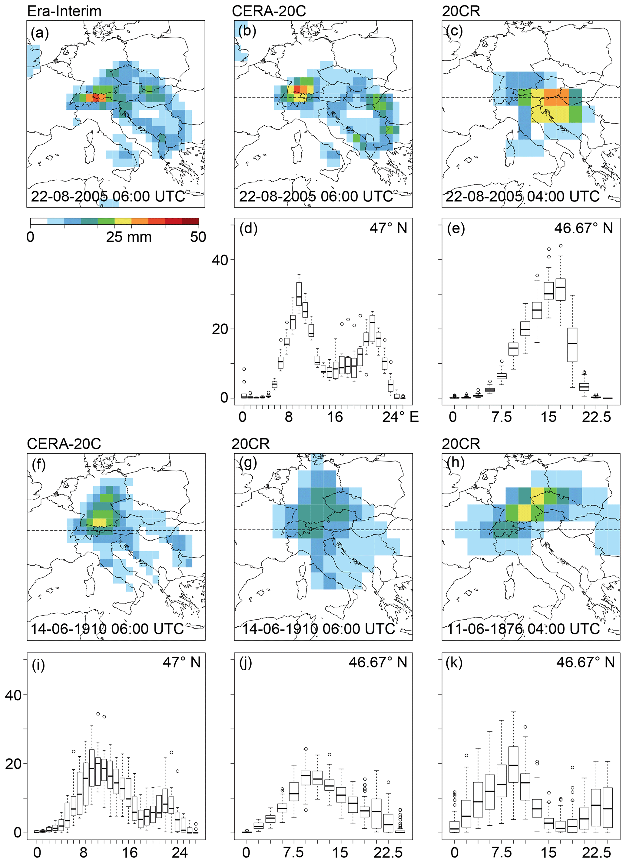
Figure 2Daily precipitation totals (mm per 24 h; color shade) as calculated for 22 August 2005 (a–c), 14 June 1910 (f, g), and 11 June 1876 (h) from ERA-Interim (a), CERA-20CR (b, f), and 20CR (c, g, h). Slightly differing time steps are due to differing temporal resolutions of the reanalyses products. Boxplots below the map panels show, respectively, and where applicable, the variability of daily precipitation totals of all ensemble members in grid boxes along cross sections at 47∘ N (CERA-20C; d and e) or 47.67∘ N (20CR; e, j, and k). The horizontal lines in (b, c, f, g, h) delineate these cross sections.
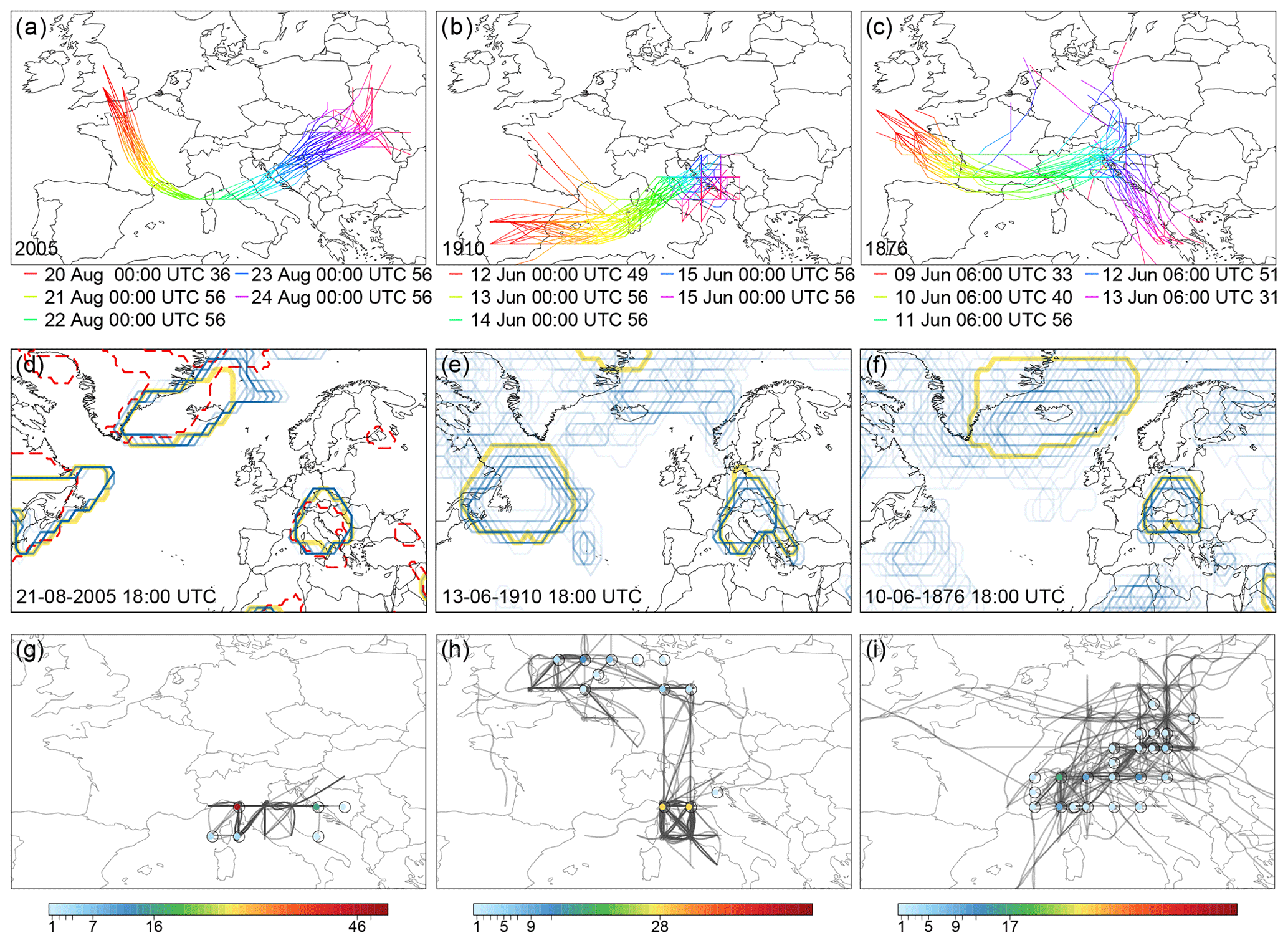
Figure 3Synoptic situations as depicted in the 20CR ensemble for the 2005, 1910, and 1876 cases. (a–c) Cyclone tracks for each ensemble member of 20CR at a mid-tropospheric, i.e., the 500 hPa, level. The color of the lines corresponds to the time steps indicated below the panels. In addition, the number indicates for how many of the 56 members a cyclone position could be reconstructed at a certain time step. (d–f) Objectively identified cyclone fields (calculated for sea level pressure; using Wernli and Schwierz, 2006; see also Welker and Martius, 2015) in the 20CR ensemble (blue contours) and 20CR mean (yellow contours) at the time steps of (d) 21 August 2005 18:00 UTC, (e) 13 June 1910 18:00 UTC, and (f) 10 June 1876 18:00 UTC. The color scheme, ranging from light blue to dark blue, indicates in how many of the 56 ensemble members a cyclone is detected in the respective grid cell. The red broken lines in the 2005 panel indicate the cyclone field as calculated from ERA-Interim. (g–i) Cyclone centers identified for sea level pressure at (g) 21 August 2005 18:00 UTC, (h) 13 June 1910 18:00 UTC, and (i) 10 June 1876 18:00 UTC, the same time steps as in (d–f). Colored dots and the tick marks in the color key indicate the number of cyclone tracks located at a specific grid point at the respective time steps. Gray scale lines mark the cyclone tracks over the period of 48 h before to 48 h past the respective time steps. Darker (lighter) gray shades indicate more (less) cyclone tracks along a certain path.
For the analyses, we use both sea level pressure (SLP) and mid-tropospheric pressure fields. SLP fields inform us about the quality of the assimilation process in 20CR, and the isobaric pressure fields (at 500 hPa here) tell us about the derivation of upper-air variables from the SLP information in 20CR. Combining SLP and isobaric levels has been found useful for cyclone tracking (Hofstätter and Blöschl, 2019; Hofstätter et al., 2016): while SLP tracks and fields accurately mark the “footprint” of a cyclone, surface pressure patterns are also modulated by (model) orography and boundary layers and can therefore behave as more short-lived patterns and be erratic in space. In this respect, pressure patterns at mid-tropospheric levels are smoother and thus more robust over space and time.
The cyclone tracks shown in Fig. 3a–c are reconstructed as follows: in a first step, absolute minima of the 500 hPa geopotential height are inventoried. Then, the cyclone centers (here, the absolute minima of geopotential height) closest to Corsica on 22 August 2005, 13 June 1910, and 11 June 1876 are selected. In a third step, cyclone tracks are reconstructed every 6 h backward and forward in time by selecting the closest cyclone position and starting from the three selected cyclones. The tracks are terminated if the cyclone position jumps over more than approximately 1200 km in 6 h. For example, an absolute minima of the 500 hPa geopotential height (here, a cyclone center) exists in 36 of the 56 ensemble members over southern England on 20 August, 00:00 UTC (Fig. 3a). One day later, all 56 members contain a cyclone center over southern France. For comparison to the mid-tropospheric level, cyclone fields (Fig. 3d–f) and tracks (Fig. 3g–i) are also calculated for SLP according to Wernli and Schwierz (2006; see also Welker and Martius, 2015). The algorithm detects cyclone fields in terms of a finite area around a regional SLP minimum, that is, by a closed SLP contour line. The regional SLP minima for each cyclone life cycle are stored as cyclone tracks, and the presence or absence of a cyclone is represented in a binary field for each grid point and time step.
Inferring from Fig. A1, as well as from analyses of supra-national rain gauge measurements (Frei, 2006; Stucki et al., 2012) or model simulations (Langhans et al., 2011, for the 2005 case), most precipitation is expected to accumulate over northeastern Switzerland and to reach well into Austria and southeastern Germany along the Alpine bow during these three cases. A second area of heavy precipitation is expected to stretch from the southeastern Alps into the Dinarides (Dinaric Alps). From these similarities, it can also be assumed that the synoptic fields of precipitation look similar for all three cases. Similarity is also presumed regarding the location and intensity of the rain-associated cyclones and cyclone tracks, as they strongly determine whether heavy precipitation is advected to the expected regions along the northeastern Swiss Alps.
For 2005, both ERA-Interim and CERA-20C produce a center of heavy precipitation (up to 50 mm per 24 h) in the expected region (Fig. 2a and b), and tongues of heavy precipitation reach east and southeast along the Alpine bow and along the Adriatic coast. In comparison, 20CR shows only one coherent, but larger, center of precipitation that is shifted towards the southeast and has lower intensity, representative for larger grid boxes (up to 35 mm per 24 h; Fig. 2c). Variability in precipitation totals among the 56 members of 20CR is larger (interquartile range of approx. 10 to 15 mm per 24 h) than among the 10 members of CERA-20C (interquartile range of up to approx. 10 mm per 24 h; Fig. 2d and e). The cyclone fields of the 2005 case, as well as the associated cyclone tracks south of the Alps, are well defined in the 20CR ensemble: shifts on only a couple of grid cells occur (Fig. 3a, d and g). For instance, 46 members show a cyclone track at 44∘ N, 10∘ E for 21 August 2005 18:00 UTC. Differences to the cyclone fields in ERA-Interim are also mostly within the range of the 20CR members.
For 1910, the centers and tongues of heavy precipitation have a similar location to 2005 in CERA-20C; although intensities are lower (up to 30 mm per 24 h). The 20CR also shows similar centers of heavy precipitation, while intensities in 20CR are clearly lower (Fig. 2f and g). In contrast, the variability among the members is higher in the CERA-20C dataset (up to approx. 10–15 mm per 24 h compared to below 10 mm per 24 h in 20CR; Fig. 2i and j). Compared to the 2005 case, the range of calculated cyclone tracks and cyclone fields for 1910 becomes larger in 20CR and encompasses three or sometimes even more grid points (Fig. 3b, e and h). A total of 56 cyclone tracks are found at two grid points (44∘ N, 10∘ E and 44∘ N, 12∘ E) for 13 June 1910 18:00 UTC.
For 1876, only 20CR is available (Fig. 2h and k) to assess the representation of synoptic precipitation fields. Compared to 1910 and 2005, the center of heavy precipitation is located more to the northeast of Switzerland, over southeastern Germany. Intensities are higher than for 1910 and lower than for 2005. Although the cyclones pass across the Ligurian Sea and northern Italy in the 2005 and 1910 cases, the bulk of the ensemble takes a more northerly path in the 1876 case (Fig. 3c, f and i). Some of the 25 members show a cyclone track at two grid points just south of Switzerland (46∘ N, 10∘ E and 46∘ N, 12∘ E). And while a small part of the members tracks towards the north or northeast on 12 and 13 June 1876, the rest show a southeastward propagation along the Adriatic Sea.
Overall, the analyses at synoptic scales (Figs. 2 and 3) show that differences among the 20CR members are substantially smaller over the region of interest (Southern and Central Europe) than over other regions of the North Atlantic or European sectors (Fig. 3d–f); this corresponds to the relatively high density of assimilated stations over central Europe (not shown; see Compo et al., 2015). The main fields of precipitation are approximately co-located in all three datasets (Fig. 2). Variability in the 20CR ensemble is comparable to CERA-20C for the 2005 and 1910 cases. 20CR shows overall lumpier spatial patterns of heavy precipitation and lower values due to the coarser horizontal grid and a potential displacement of the precipitation field for the 1876 case. As expected, the uncertainty, in terms of disagreement between the 20CR ensemble members, becomes increasingly larger when going back in time. For instance, the cyclone fields and cyclone tracks over the Alpine area are only a little less well defined for 1910 compared to 2005, but much less for 1876. Among others, this is shown by the number of co-located cyclone tracks (in terms of pressure minima) in the 20CR ensemble. The algorithm detects 56 co-located cyclone tracks at a grid point over northern Italy on 21 August 2005 18:00 UTC (Fig. 3g). For the time step 13 June 1910 18:00 UTC (Fig. 3h), 56 cyclone tracks are detected at two adjacent grid points, whereas only 17 co-locations are found for 10 June 1876 18:00 UTC (Fig. 3i). From these analyses, we infer a very good to satisfactory positioning of cyclone tracks and cyclone fields in 20CR for the 2005 and 1910 cases, but not necessarily for 1876. This means that the boundary and initial conditions appear to be captured in 20CR for the 2005 and 1910 cases, while 1876 shows two or even more potential developments of the cyclone.
4.2 Precipitation, cyclone tracks, and moisture transport along the downscaling steps
In this section, we examine how well the three Vb cases are represented when downscaling the global information from 20CR to a 3 km horizontal grid using the WRF regional model. In the first place, we analyze the variability of precipitation totals in the downscaled ensemble for all three cases, with a special focus on the contribution of convection. Secondly, we address flow features along the downscaling steps which explain contrasting (very large or very small) precipitation totals in the simulations. To conclude the analyses, we use an exemplary member of the 1910 case to illustrate how a specific pattern of cyclonic flow translates into characteristic near-surface weather during heavy-precipitation Vb events over the Central Alps.
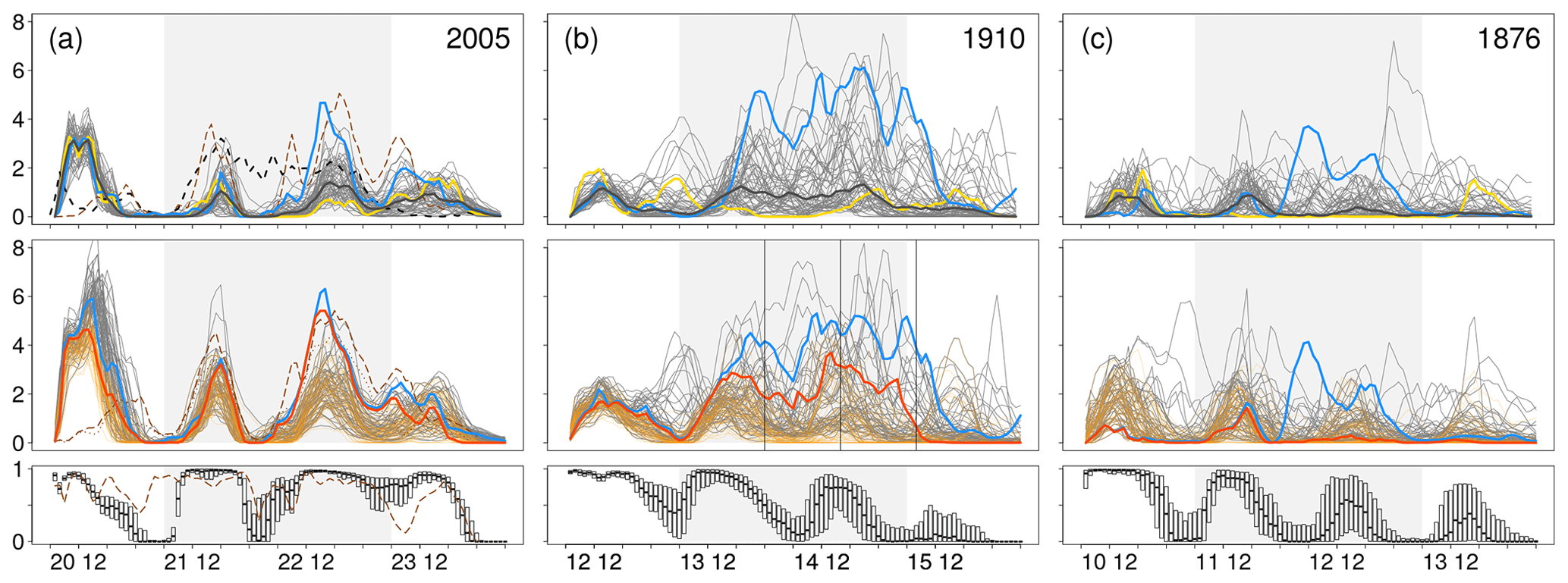
Figure 4Time series of simulated precipitation over northern Switzerland for (a) 20 August 2005 06:00 UTC to 24 August 2005 06:00 UTC, (b) 12 June 1910 06:00 UTC to 16 June 1910 06:00 UTC, and (c) 10 June 1876 06:00 UTC to 14 June 1876 06:00 UTC. Dark gray lines indicate mean hourly precipitation (mm h−1) within the control area over northern Switzerland for the 56 downscaled ensemble members, as simulated for the 3 km domain (upper panels) and the 9 km domain (middle panels). In the upper panels, the thick black (yellow, blue) solid lines mark the median (minimum-precipitation, high-precipitation) members, as selected for Figs. 5 to 8 and Fig. 10. In the middle panels, thin orange lines show the contribution of the convection parametrization to the total precipitation in the 9 km domain. The thick dark orange lines indicate convective precipitation for the selected high-precipitation members. The bottom panels show the proportion of convective precipitation with respect to total precipitation in the 9 km domain. In panel (a), the dashed black line shows the corresponding hourly precipitation calculated from CombiPrecip, and the dashed brown lines show the precipitation from the ERAI-WRF experiment with 4 domains; the convective contribution is shown with points in the middle panel. Black vertical lines in (b) indicate the instances in time selected for Fig. 10. Gray shadings mark the most intense 48 h periods of precipitation according to Fig. A1.
In the first analysis, we address the temporal variability of the simulated precipitation. Figure 4 shows time series of aggregated precipitation in the control area over northern Switzerland. In the 2005 case (Fig. 4a), two distinct peaks occur on 21 and 22 August 2005 around 18:00 UTC. This evolution is very much in line with Hohenegger et al. (2008; their Fig. 8); even the increase during the second peak episode is very similar. Intensities are mostly underestimated when compared to CombiPrecip. Arguably, too little precipitation is produced between the simulated peak episodes, although more intermittent precipitation was also observed in a (smaller) area over eastern Switzerland (Hohenegger et al., 2008), and CombiPrecip may as well be imperfect over the control area. Two high-precipitation episodes are also simulated for 1910 and 1876 (Fig. 4b and c), although variability among the members increases regarding the timing and intensities of precipitation. For instance, the ensemble interquartile range is smallest for 2005 (around 1.5 mm h−1 in the peak episode; note that this is smaller than in Hohenegger et al., 2008) and becomes larger for the earlier cases (around 2 mm h−1 on 14 June 1910 18:00 UTC and around 2.5 mm h−1 on 11 June 1876 18:00 UTC).
For all cases, the ensemble shows most precipitation peaks in the afternoon. This would be in agreement with an enhancing effect by (embedded) convection. To investigate this effect, we turn to the second-finest domain with a 9 km horizontal grid. Whereas convection is explicitly simulated for the 3 km domain, it is parameterized in the 9 km domain, resulting in WRF model variables of nonconvective (RAINNC) versus convective (RAINC) contributions to the total precipitation (the shallow convection variable RAINSH is turned off). For the 2005 case and in the 9 km domain, convective precipitation is the largely dominant process during the afternoons (Fig. 4a), reaching nearly 100 % in all the members and on all days of the event. The proportion of convective precipitation is smaller during other times of the day and varies more in the ensemble. The same pattern is found for the 1910 and 1876 cases, although the proportion of convective precipitation is mostly smaller and variability in the ensemble is higher (Fig. 4b and c).
Peaks of precipitation are also simulated during the initialization period of each case, which is in line with observations (not shown; cf. Stucki et al., 2012). However, the peak on 20 August 2005 is too prominent compared to CombiPrecip (Fig. 4a). The convection-driven peak is simulated for all members including the minimum-precipitation member, while precipitation intensity appears more realistic in the WRF-ERAI simulation. One explanation might be found in the coarser interpolation from 20CR input data (from 220 km grids compared to 80 km in ERA-Interim), which results in too high temperatures over the Alps for this specific case. In turn, this may lead to enhanced convection over this area and during the first hours of the 20CR-WRF simulation (not shown).
Next, we examine whether the found features and variabilities in the ensemble reflect differences that are already present in the 20CR members (Fig. 2) or if they appear along the downscaling steps. Concretely, we search for flow features that help to systematically distinguish members with low or high precipitation simulated in the correct region (i.e., in the control area over northeastern Switzerland). For this, we compare the simulated 48 h precipitation totals with RrecabsD. We use the ratio of precipitation in the simulation versus the reconstructions and the EMD between simulation and reconstruction to assess the similarity of the spatial distribution of precipitation.
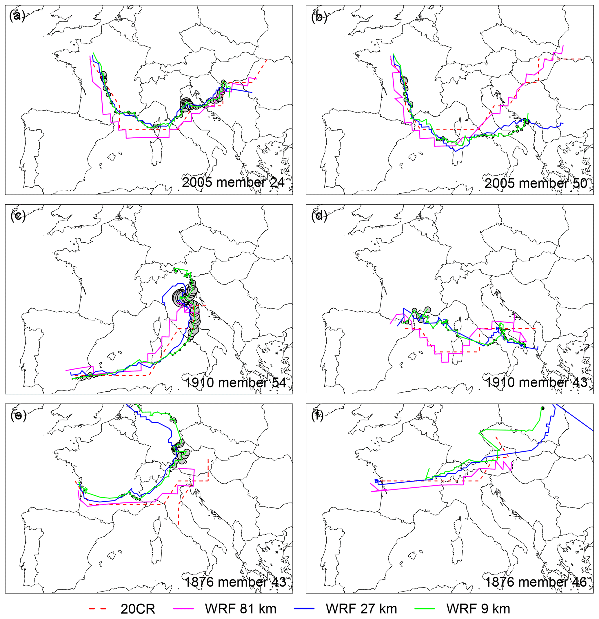
Figure 5Cyclone tracks, calculated for 500 hPa levels, for the cases of 2005 (a, b), 1910 (c, d), 1876 (e, f), and for members producing maximum (a, c, e) and minimum (b, d, f) precipitation totals over northern Switzerland. The cyclone tracks in 20CR and WRF at 81, 27, and 9 km grid sizes are shown in red, magenta, blue, and green, respectively. Filled circles indicate the mean hourly precipitation over northern Switzerland at the time step when the cyclone was centered at the respective grid point in the WRF 3 km domain. The circle diameters grow linearly with the precipitation amounts; the largest circle (in c) represents 6.6 mm h−1.
For illustration, the panels in Fig. A3 show (i) a maximum member in terms of simulated precipitation (a near-maximum member is chosen for the 1876 case because the maximum member does not show plausible patterns, cf. Fig. 4c) and (ii) a minimum member in terms of lowest precipitation totals in the control area. Indeed, the two contrasting members are exemplary for the large variability of the simulation results. Throughout the ensemble, we find members that largely misestimate the precipitation totals (the range is around 20 % to 160 % for the 2005 and 1910 cases and 5 % to 70 % for the 1876 case, not shown), while others produce precipitation at the wrong place but also a number of members that produce quite accurate spatial patterns and precipitation totals compared to observations and the RrecabsD reconstruction.
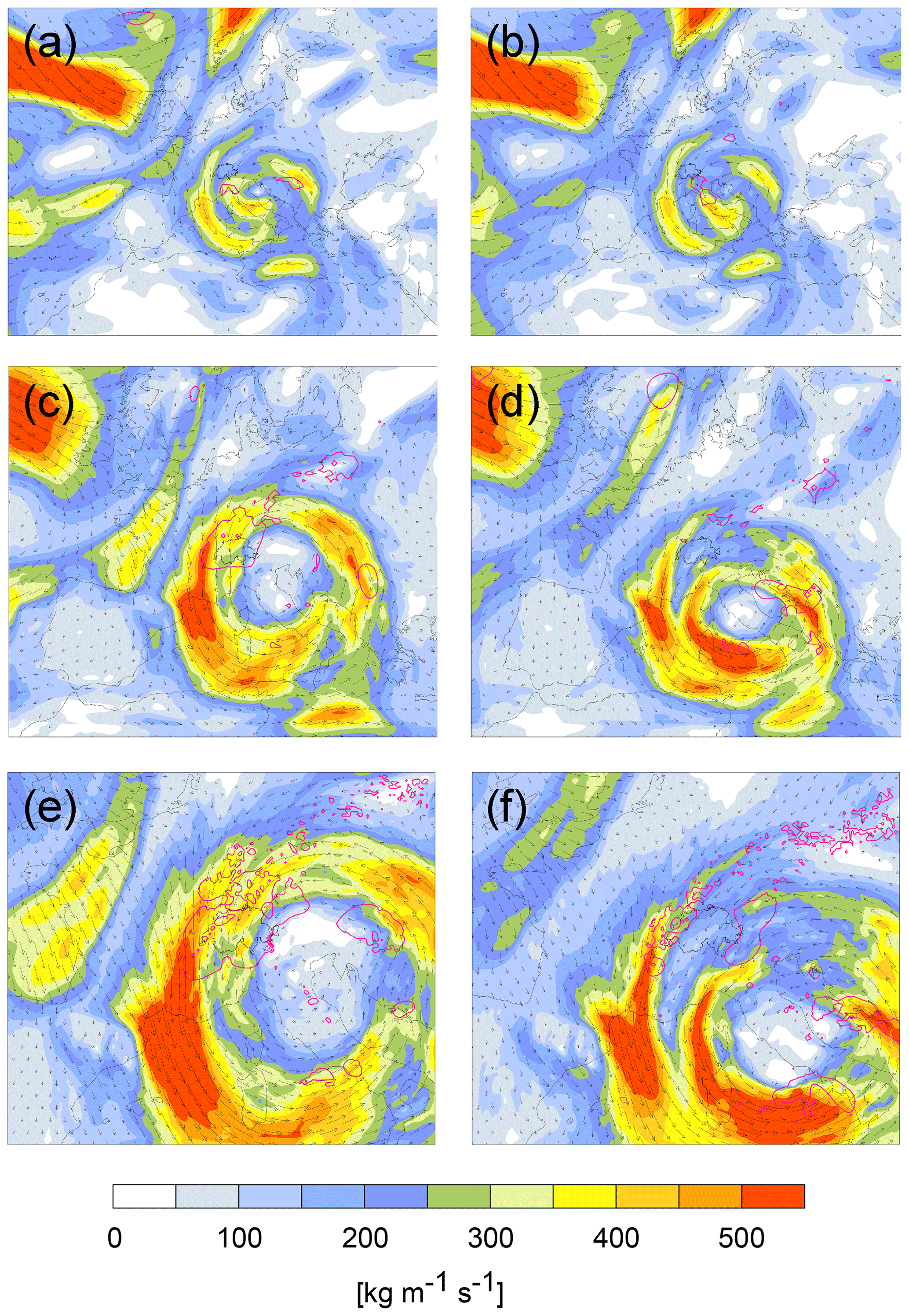
Figure 6IVT (kg m−1 s−1) on 22 August 2005 18:00 UTC for in the WRF 81 km (a, b), 27 km (c, d), and 9 km (e, f) domains and for a member producing maximum (#24; see Fig. A2; a, c, e) and minimum (#50; b, d, f) precipitation totals. Smoothed hourly precipitation is shown with pink contours of 0.2 and 1 mm h−1.
Figure 5 delineates the corresponding evolution of the cyclone tracks in selected ensemble members that yield maximum (Fig. 5a) or minimum (Fig. 5b) precipitation for the 2005 case. The cyclone track for the maximum-precipitation member follows closely the original cyclone track in 20CR in each downscaling step. During the peak episode, the cyclone center is located just above the Adriatic coast of northern Italy. Moreover, the multiple circles at the same location (Fig. 5a) indicate the quasi-stationarity of the cyclone. In contrast, the minimum-precipitation member has a cyclone track in the 27 km domain that clearly departs from the original 20CR cyclone track: instead of recurving to the north over Italy, it keeps propagating eastward. The high-resolution domains (9 and 3 km, not shown) then represent refinements of these patterns without significant changes. In the 1910 case, the cyclone tracks for the maximum-precipitation member (Fig. 5c) also show in the vicinity when compared to 20CR in all downscaling steps, recurving to the north and the same location during stalling, i.e., peak episode. In contrast, the minimum-precipitation member shows a more southerly and eastward track after it reaches Italy (Fig. 5d). That is, the tracks of 20CR and the coarsest downscaling step never turn towards the north, thus making it more difficult to bring precipitation towards the target area. In contrast to the 2005 and 1910 cases, the algorithm has difficulties to detect clear cyclone tracks along the downscaling steps for the 1876 case (Fig. 5e and f). In addition, the found tracks run just south of or even across Switzerland, hence on a much more northerly path than for the other two cases. Such tracks do no longer represent a typical Vb trajectory.
The panels in Fig. 6 (for the 2005 case), Fig. 7 (for 1910), and Fig. 8 (for 1876) illustrate the link between the exact position of the cyclone track and the moisture transport in terms of IVT, showing variations of synoptic-to-mesoscale features along the downscaling steps for the simulated peak times. In the 2005 case, the IVT patterns of the vortex located southeast of Switzerland are very similar among the two contrasting members in 20CR (not shown), and small differences appear in the 81 km domain (Fig. 6a and b). This changes in the 27 and 9 km domain (Fig. 6c and d): in line with the cyclone track in Fig. 5, the IVT vortex of the minimum-precipitation member is clearly shifted towards the south. The location of the cyclone center strongly determines the intensity of the moisture flux and precipitation over the Alps: in the maximum-precipitation member in Fig. 6e, moisture is transported all the way around the Alpine chain. For the minimum-precipitation member in Fig. 6f however, the circle of intense IVT around the cyclone center is shifted to the south and is moreover partly interrupted over the northern Alps and Switzerland, arguably because a lot of the moisture already precipitates upstream, i.e., over the Dinarides in the Balkans.
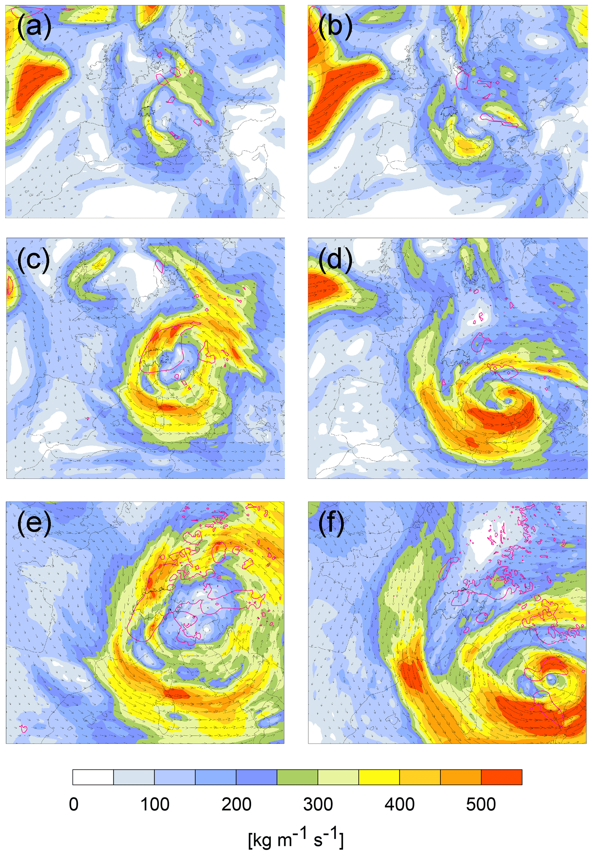
Figure 7As in Fig. 6, but for 14 June 1910 18:00 UTC, and for different maximum (#54) and minimum (#43) members.
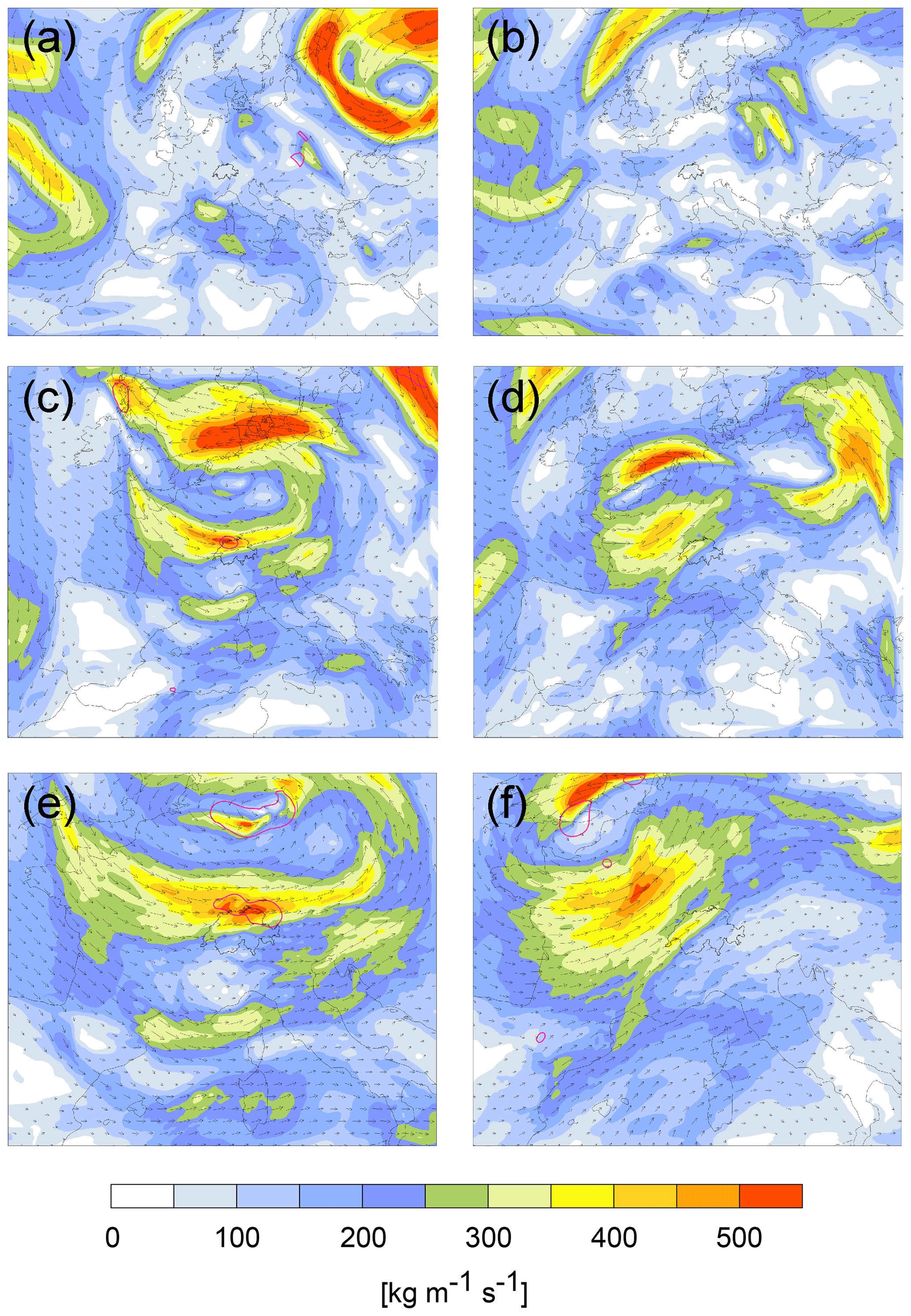
Figure 8As in Fig. 6, but for 13 June 1876 00:00 UTC, and for different maximum (#43) and minimum (#46) members.
In the 1910 case (Fig. 7), the corresponding patterns of the IVT vortices are very similar to the 2005 case, although showing lower intensities over the Alps in 20CR (not shown) and the 81 km domain. The maximum-precipitation member shows northerly winds and intense moisture flux and precipitation over Switzerland, associated with the cyclonic IVT pattern surrounding the cyclone center (Fig. 7c and e). In the minimum-precipitation member however, the cyclone center and associated cyclonic IVT pattern are shifted southeastwards, such that the intense IVT misses the Central Alps (Fig. 7d and f). In the 1876 case (Fig. 8), the maximum-precipitation member features hardly any structures of a vortex in 20CR (not shown) and in the 81 km WRF domain, and the IVT vortex appears broken and misplaced at higher resolutions. A center of the cyclone is located over northern Germany and induces intense moisture transport in a westerly flow. Hence, some areas in northern Switzerland receive intense precipitation, although it is not anymore associated with a classical Vb cyclone. In the minimum-precipitation member, the cyclone center is also located to the north but also to the west of Switzerland (Fig. 8d and f). Again, Switzerland is on the south side of the vortex, within a southwesterly moisture flux reaching into western Switzerland only and missing most of the Central Alps.
Furthermore, Fig. 9 demonstrates that indeed, precipitation intensity over northern Switzerland was closely related to the intensity and direction of the moisture transport towards the Alps during the heavy-precipitation phase of the three cases. In the 2005 and 1910 cases (Fig. 9a and b), IVT intensities of more than 200 kg m−1 s−1 are advected from northwest to northeast (i.e., directed towards the northern side of the Alps). This is concurrent with average precipitation rates of up to 8 mm h−1, whereas precipitation rates become clearly lower with decreasing IVT and with other inflow angles, as seen in the 1876 case (Fig. 9c). Similar results were found by Froidevaux and Martius (2016).
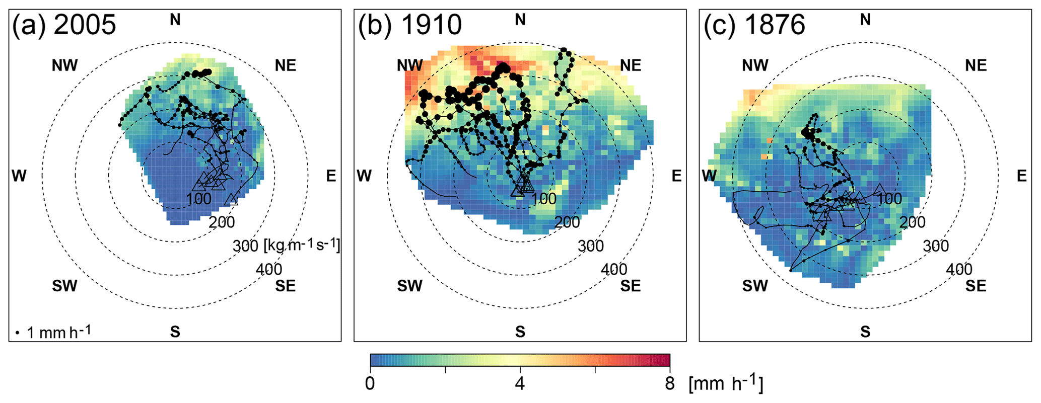
Figure 9Hourly precipitation (mm h−1; color shade) as a function of IVT (kg m−1 s−1; dashed circles) over northeastern Switzerland during 48 h periods starting at (a) 21 August 2005 06:00 UTC, (b) 13 June 1910 06:00 UTC, and (c) 11 June 1876 06:00 UTC. Both precipitation and IVT are averages over the control area in northeastern Switzerland in the 3 km WRF domain. The 480 black dots represent 48 different time steps for a subset of 10 members (see Sect. 3.1). The size of the dots represents precipitation intensity; the location of the dots on the radial diagram represents IVT: the azimuth represents the direction of IVT and the radial component its intensity. All time steps of a same member are connected by a line, with the last time step marked by a triangle. The corresponding two-dimensional interpolation of the precipitation intensity is shown in color. The color maps hence represent the mean precipitation intensity as a function of IVT intensity and direction.
In summary, the 2005 and 1910 cases behave similarly along the downscaling steps in the simulation, whereas the 1876 case deviates in a range of aspects. In the 2005 and 1910 cases, Vb cyclones exist for all members in 20CR (Figs. 3 and 5), and the cyclone centers cross the WRF domains at 81, 27, and 9 km grid sizes. In the 3 km domain, the trajectory of the cyclone centers typically passes southwards of the domain, and a clear cyclonic circulation is systematically present, corresponding to the position of the cyclone in the 9 km domain (Figs. 6–8). This can be expected, as the cyclone is larger than the two smallest domains, which hampers shifting of cyclone centers. Moreover, we find that the cyclones with centers that stall over a specific location of northern Italy and/or the Adriatic Sea are associated with more intense precipitation over northeastern Switzerland. The maximum-precipitation simulation for 1910 produces even larger totals than observed (Fig. 4; see also Figs. 7, 9 and A3). This may indicate that under slightly different atmospheric conditions, e.g., with longer stalling of the cyclone at a particularly unlucky location, the real cases could have had even worse impacts.
In contrast, members with more southerly tracks do not produce heavy precipitation in this region. With a displacement to the south, the moisture transport does no longer provide a northern inflow towards the Alps, which then inhibits the orographic lifting along the Alps (Figs. 6–8 and A3). Hence, the moisture removal from the atmosphere is limited, leading to less precipitation in general and especially in the target area.
Too northerly tracks are not helpful in generating plausible precipitation patterns either. The 1876 case shows that the vortex structure is destroyed as soon as the cyclone centers are located too close to the Alps. Instead of intense moisture advection from a northern sector, advection on the north side of the Alps shifts to a western or even southern sector. This behavior of the model can be explained by the interaction of the Alpine orography with atmospheric circulation. Indeed, Vb cyclone trajectories are typically initiated by deepening upper-level troughs, which finally cut off from the westerly flow when passing over the Alps (e.g., Awan and Formayer, 2017). The interaction of upper-level troughs with the Alpine orography has been described in detail (Buzzi and Tibaldi, 1978; Aebischer and Schär, 1998; Kljun et al., 2001); the underlying processes include flow splitting and lee cyclogenesis, with further amplifications of the cyclone formation by frontal retardation and latent heat release due to orographic lifting. The combination of these processes implies that the cyclones are formed on the lee of the right side of the Alps, typically over the Ligurian Sea. In 20CR, however, the Alpine orography is very coarse, smoothed, and reaches only about 1000 m a.s.l. (cf. Stucki et al., 2012). Hence, the influence of the Alps on the large-scale flow is limited in 20CR. Given also that the 1876 case is least confined by pressure observations, this allows untypical cyclone tracks in many 20CR members. Once accounting for a more and more realistic orography throughout the downscaling steps with WRF, the high-resolution runs may thus end up in a compromise simulation – driven both by the WRF model physics and by the 20CR input flow. In other terms, the large-scale flow forced from 20CR might not be compatible with the orography of the high-resolution domains.
To conclude the analyses, Fig. 10 illustrates how a certain combination of cyclone tracks and cyclonic moisture flux translates into a specific weather situation at the surface. For this, we select the maximum-precipitation member (#54) for the 1910 case and show an early, mid, and late instance of the heavy-precipitation period (cf. Fig. 4), and we compare it with findings regarding the 2005 case.
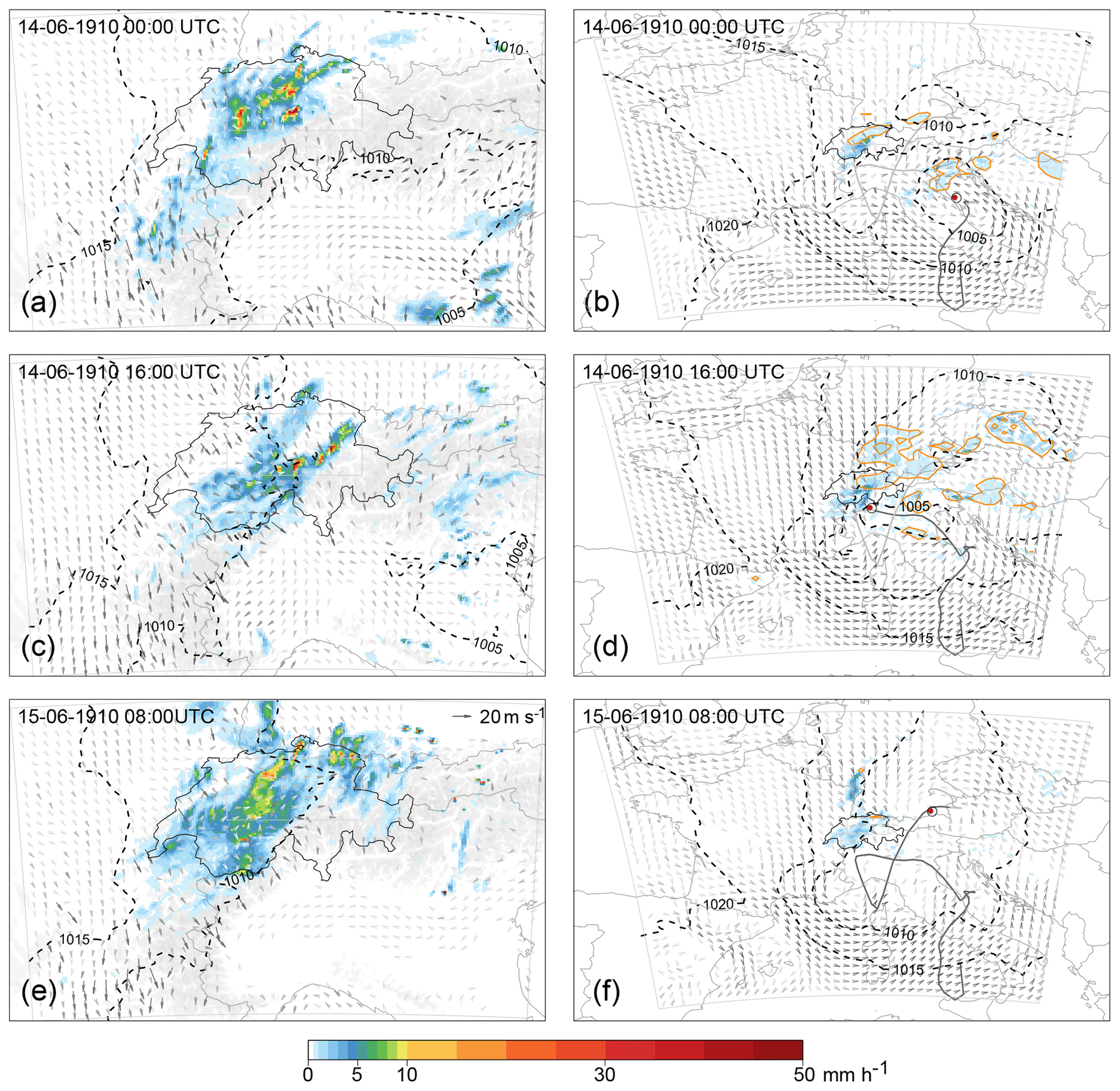
Figure 10The 1910 event (as shown in the downscaled member #54) in the 3 km WRF domain (a, c, e) and corresponding 9 km WRF domain (b, d, f) and for three instances in time corresponding to heavy precipitation over northern Switzerland, that is, at (a, b) 14 June 1910 00:00 UTC, (c, d) 14 June 1910 16:00 UTC, and (e, f) 15 June 1910 08:00 UTC. Shown are hourly precipitation (mm h−1; color shade), 10 m wind field (m s−1, light gray vectors darken with increasing velocity, see reference vector of 20 m s−1 in e), and SLP (dashed contours, in 5 hPa increments). In (b, d, f), orange contours show the contribution of the convection parameterization to the total precipitation (contours at 2 and 5 mm h−1). The dark (light) gray lines in the 9 km domain indicate the smoothed cyclone track starting on 13 June 1910 00:00 UTC and until the shown instance. The red dot marks the cyclone center (i.e., pressure minimum) at the respective instance in time.
For 14 June 1910 00:00 UTC, the 3 km downscaling shows patches of heavy precipitation along the Alps and Alpine foothills of northern Switzerland (Fig. 10a). Many of them appear in banded structures, similar to findings from the 2005 case (Bezzola and Hegg, 2007; Langhans et al., 2011). The structures are generally oriented parallel to the Alpine bow and reach from southeastern Germany into central Switzerland. Surface winds in the control area come from a northern to north-northwestern sector and weaken upwind of the Alpine barrier. Concurrent areas of convection appear in the 9 km simulation (Fig. 10b), and the pressure gradient along the Alpine rim shows the Vb low-pressure system over the Adriatic Sea. At the same time, the IVT vortex just starts to show intense moisture transport from the northeast towards Switzerland (not shown, cf. Fig. 6 for a later instance). In all, this indicates persistent airflow upon orography and orographic lifting, as documented for the 2005 case (Zbinden, 2005; Bezzola and Hegg, 2007) and visible in CombiPrecip and wind observations for the evening of 21 August 2005 (not shown).
On 14 June 1910 16:00 UTC, the center of the low-pressure system is located just south of Switzerland (see red dot in Fig. 10d). Accordingly, the northerly cross-Alpine flow is substantially stronger, and heavy precipitation becomes most intense along the northern Alpine ranges (Fig. 10c). Again, this shift of the heavy precipitation into the Alpine ranges with enhanced northerly flow is in line with analyses of the 2005 case (Zbinden, 2005; MeteoSwiss, 2006; Bezzola and Hegg, 2007) and with CombiPrecip and wind observations for 22 August 2005 (not shown). The 9 km simulation shows the associated areas with intense convection reaching into Switzerland from the northeast (Fig. 10d). At this stage, the cyclonic flow forms a distinct arc that stretches from the eastern to the central Alps.
On 15 June 1910 08:00 UTC, the SLP minimum has crossed the Alps to the northeast of Switzerland (Fig. 10f). In the 3 km simulation, heavy precipitation occurs in an area of southwesterly winds along the Alps, the Swiss Plateau, and towards the east, while the flow remains northwesterly at higher elevations and towards the north or northwest (Fig. 10e). Concurrently, the SLP fields in the 9 km simulation indicate higher pressure from the west, before precipitation intensifies along the eastern Alps, while it finally eases over Switzerland. This is again analogous to a late stage of the 2005 case (MeteoSwiss, 2006; Bezzola and Hegg, 2007; Fig. 10f), e.g., visible in CombiPrecip and wind observations for around midnight on 22 August 2005 (not shown).
In the end, all simulated instances are associated with heavy precipitation over northern Switzerland, with slight changes in the inducing weather dynamics. In the first instance, banded convection and orographic lifting both contribute to intense precipitation. The second instance, corresponding to the peak precipitation, is associated with stronger northerly winds and a distinct cyclonic moisture flux around and over the Alps. The last instance is linked to a shift towards westerly advection and increasing pressure. While the early stage of the SLP cyclone track calculated for member 54 is not very typical (no cyclogenesis in the classic Genoa region; see Fig. 5c), the surface analyses of the two innermost domains during the heavy precipitation phases show that the simulation produces realistic near-surface weather dynamics at local scales, and they can clearly be related to the circulation and features of a Vb cyclone.
In this study, we have assessed the potential of dynamical downscaling from 20CR input to 3 km grid sizes for three well-known Vb cyclones that led to heavy precipitation and flooding in (northeastern) Switzerland in August 2005, June 1910, and June 1876. In particular, we have analyzed the sensitivity of the produced precipitation totals in a control area in northeastern Switzerland to (i) the setup of the regional weather model and to (ii) the representation of moisture flux in the 20CR ensemble and along the downscaling steps.
Regarding the configuration of the regional weather model (WRF in our case), we have found for our purposes that short spin-up periods (encompassing around 24 h before the heavy-precipitation episode) are preferable over long spin-up periods, which would allow (partial) adaptation of small-scale and slow-reacting variables in the model, such as soil moisture, for instance. In our experiments, precipitation totals in the ensemble become less variable and more realistic if the cyclones are already present in the outermost model domain at model initialization; if not, the simulation runs too freely. Other than that, substantial changes in standard physics options do not increase model performance, be it cumulus or micro-physics or two-way nesting. Given that the cumulus parameterization is turned off for the 9–3 km downscaling step, comparable outcomes with differing physics schemes point to the importance of the larger-scale atmospheric flow for producing the heavy precipitation. Although we find no relevant enhancements from nudging in smaller domains in our test experiments, nudging smaller domains could still be beneficial for other specific studies. In the simulations of the cyclonic vortex, the largest deviations along the downscaling steps occur in the 27 km domains. The increasing variability of the simulations in these domains might be explained by the fact that no nudging is applied, while it is in the larger, 81 km, domains. Although going back far in time, we have only analyzed a very small number of events – many more cases would be needed to reach robust recommendations on how to configure a model for Vb cases. Nevertheless, we have demonstrated that one can achieve a relatively good configuration for the desired application with a well-thought series of experiments.
In our context, the EMD has proven to be a valuable and intuitively understandable tool for spatial verification of the simulated precipitation fields with observation-based reconstructions. In fact, our EMD analysis results in similar rankings as obtained from the more common spatial verification scores and metrics (MAE, box ratios; see Table 2) or from intersubjective, visual analyses of the precipitation patterns.
Regarding the representation of precipitation and related variables in the 20CR ensemble, we find that 20CR delivers a well-confined ensemble for the 2005 case. Given the coarser horizontal grid sizes and lower vertical resolution, it compares well with other long-term reanalysis products. The 1910 case is also comparably well defined in the 20CR ensemble, whereas the 1876 case shows more uncertain developments of the cyclone fields in the ensemble. This gradually increasing uncertainty when going back in time is also found for precipitation-related variables along the downscaling steps. For instance, the dynamical downscaling procedure captures the peak episodes of all three cases, although gradually less well going back in time. Furthermore, the accuracy of precipitation totals is closely linked to the exact cyclone track and the exact location of the vortex when it comes to stalling. Concretely, this location should be over northern Italy, or just off the northern Adriatic coast for best simulation results with regards to the intensity and spatial distribution of precipitation totals over northeastern Switzerland.
Ensemble members that do not follow such a trajectory produce erroneous precipitation totals in the control area, where too southerly tracks generally produce too little precipitation, and too northerly tracks lead to a break-up of the associated vortices because of interaction with the Alpine (model) topography. This is found to be a decisive element, because the exact (stalling) location of the vortex strongly influences the cyclonic moisture transport around the Alps and the exact inflow angle from a northern sector to the Central Alps. In fact, IVT intensities of >200 kg m−1 s−1 or even more from the right direction are needed to reproduce the extreme events. Interestingly, we have found a range of members that produce more precipitation than observed and reconstructed for the 1910 case. We infer that with a slightly different, hence ideal, constellation of the cyclonic vortex, e.g., a longer stalling at the right location, even heavier precipitation over northern Switzerland could have been produced, and the 1910 floods could have had even worse impacts.
Misplacement of the vortex increase in the ensemble from the 2005 to the 1910 and 1876 cases. While the patterns and dynamics can be reproduced for the 2005 case and, a bit less well, for the 1910 case with downscaling from 20CR, the variability of the cyclone fields and tracks becomes very large in the 20CR ensemble for the 1876 case. As a consequence, we find synoptic patterns in some members that are substantially different from the 2005 case, e.g., with some cyclone tracks that do not anymore follow a typical Vb path anymore. Furthermore, the increasing uncertainties in the ensemble going back in time are also due to the decreasing quality and amount of assimilated pressure data in 20CR. For illustration, the total number of stations assimilated in 20CR in the year 1876 is 218 (Compo et al., 2015). This number grows to 377 in the year 1910 and to 9251 in the year 2005. Of course, this uncertainty propagates into our downscaled ensemble. In turn, this means that with the 1876 case, we may have reached the limits of downscaling from the current 20CR (version 2c with a 2∘ by 2∘ horizontal grid) for such complex weather situations. The WRF regional model requires more accurate locations and intensities for input variables, like cyclone fields and moisture transport, to properly reproduce such sensitive Vb cases. On the upside, we have shown that despite these deficiencies, single ensemble members, even from the early cases, can be used to analyze and illustrate local-scale weather dynamics, as well as sensitivities of the precipitation over northern Switzerland to the evolution of the associated Vb vortex.
The question of whether a full ensemble needs to be downscaled to gain such insights remains. Generally speaking, the benefit from downscaling all 20CR members is that we obtain a full set of propositions for local weather patterns during historical events. In terms of impact and intensities (in our case the local precipitation totals over northern Switzerland), the spread between these propositions is very large, reflecting the strong uncertainty inherent to the process of downscaling over a wide range of scales (here from 200 to 3 km). Hence, using ensemble members has allowed us to (i) compare members with observations and select realistic runs and to (ii) relate the differences among the members in local weather to a different evolution on larger scales. In hindsight however, the limitations of downscaling and the potential ranges of the precipitation-related variables may as well be predictable from the input data to some extent. In our case, the well (or, in contrast, badly) confined cyclone tracks and fields in 20CR for the 2005 and 1910 (1876) cases give a good indication regarding the prospects of success for dynamical downscaling. This means that in a case where the driving atmospheric dynamics on a large scale can be anticipated, the chances of a good reproduction of the local patterns and intensities with accordingly selected ensemble members are high (cf. Stucki et al., 2015). A second option would be to save computational costs by downscaling to an intermediate scale in the first place, assess the relevant dynamics in this domain, and then do the full downscaling with a well-reasoned selection of members. In our case, the largest deviations from the initial conditions often appear in the 27 km domain (the largest domain without nudging), if not already present in the 20CR member. This means that downscaling to the first non-nudged domain could be sufficient to assess if an ensemble detects a cyclone well. In such a way, future studies may minimize the computational efforts for downscaling from a coarsely resolved reanalysis ensemble.

Figure A1(a–c) Daily precipitation totals (mm per 24 h, indicated by color shade and circle sizes) from measurements over Switzerland, starting on (a) 22 August 2005 06:00 UTC, (b) 14 June 1910 06:00 UTC, and (c) 11 June 1876 06:00 UTC. (d–f) Reconstructions of 48 h totals starting at (d) 21 August 2005 06:00 UTC, (e) 13 June 1910 06:00 UTC, and (f) 11 June 1876 06:00 UTC, as derived from RrecabsD data. (g) Reconstruction of (g) 48 h totals starting at 21 August 2005 06:00 UTC as derived from CombiPrecip. The rectangle inset shows the smaller box (i.e., control area) used for the VarRatio, EMD, and precipitation totals; the full panel shows approximately the larger box used.
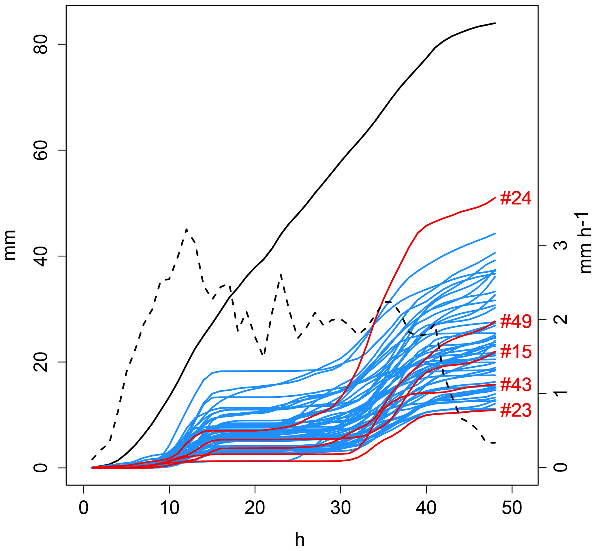
Figure A2Cumulative totals of hourly precipitation (mm, left y axis) over 48 h starting at 21 August 2005 07:00 UTC (x axis), as simulated in 56 members (blue lines) that are downscaled from 20CR. Mean values are given for a control area in northeastern Switzerland. Ensemble members (#23, #43, #15, #49, #24) representing the quartiles of the distribution are highlighted in red. For comparison, cumulative totals in the CombiPrecip dataset are shown (black line), as well as the hourly time series in CombiPrecip (dashed line; mm on the right y axis).
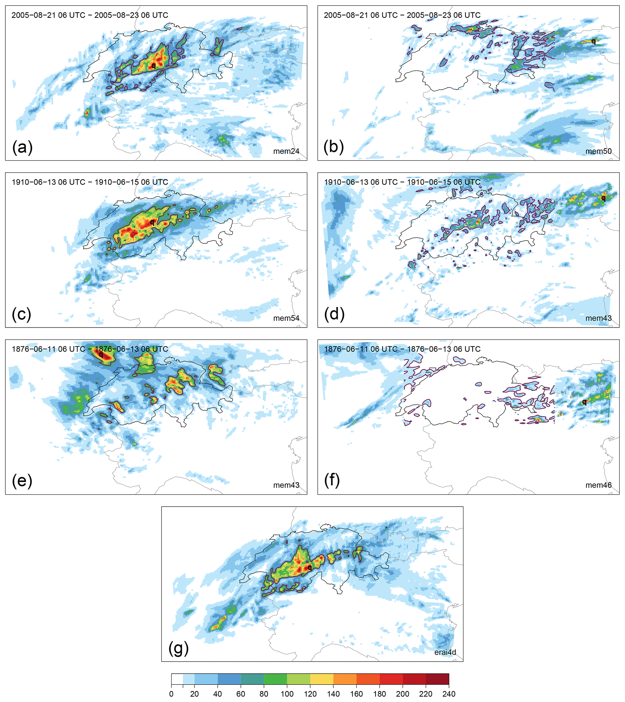
Figure A348 h precipitation totals (time periods as in Fig. A1d–f) for (a, c, e) maximum-precipitation members and (b, d, f) minimum-precipitation members for (a, b) the 2005, (c, d) the 1910 and (e, f) the 1876 cases, and for (g) the same simulation setup but with downscaling ERA-Interim for the 2005 case. Precipitation totals may be larger than 240 mm in the panels.
The WRF modeling system (Skamarock et al., 2008) source codes are in the public domain and freely downloadable from the University Corporation for Atmospheric Research (UCAR, 2020) website at https://www2.mmm.ucar.edu/wrf/users/downloads.html. The underlying research data are also publicly available. The NOAA Earth System Research Laboratory (ESRL, 2020) website at https://www.esrl.noaa.gov/psd/data/20thC_Rean/ provides access to the Twentieth Century Reanalysis dataset version 2c (Compo et al., 2011). Access to ensemble members is provided via the National Energy Research Scientific Computing Center (NERSC, 2020) at https://portal.nersc.gov/project/20C_Reanalysis/. The European Centre for Medium-Range Weather Forecasts (ECMWF, 2020) website at https://www.ecmwf.int/en/forecasts/datasets/browse-reanalysis-datasets provides access to the ERA-Interim (Dee et al., 2011) and CERA-20C (Laloyaux et al., 2016) reanalyses.
PS, PF, MZ, MM, and AM designed the experiments. MZ and MM carried them out. FAI contributed RrecabsD. PS, PF, and MZ produced the figures and tables. All authors contributed to interpretation of the analyses, particularly the spatial verification, as well as writing or reviewing the article.
The authors declare that they have no conflict of interest.
Peter Stucki and Paul Froidevaux have been supported by the Oeschger Centre for Climate Research, University of Bern. Marcelo Zamuriano has received support from the Federal Commission for Scholarships for Foreign Students through the Swiss Government Excellence Scholarship (ESKAS No. 2015.0793) for the academic year(s) 2015–2018/2019. Support for the Twentieth Century Reanalysis project dataset is provided by the US Department of Energy, Office of Science Innovative and Novel Computational Impact on Theory and Experiment (DOE INCITE) program, the Office of Biological and Environmental Research (BER), and by the National Oceanic and Atmospheric Administration Climate Program Office.
This paper was edited by Joaquim G. Pinto and reviewed by four anonymous referees.
Aebischer, U. and Schär, C.: Low-Level Potential Vorticity and Cyclogenesis to the Lee of the Alps, J. Atmos. Sci., 55, 186–207, https://doi.org/10.1175/1520-0469(1998)055<0186:LLPVAC>2.0.CO;2, 1998.
Awan, N. K. and Formayer, H.: Cutoff low systems and their relevance to large-scale extreme precipitation in the European Alps, Theor. Appl. Climatol., 129, 149–158, https://doi.org/10.1007/s00704-016-1767-0, 2017.
Baker, L. H., Gray, S. L., and Clark, P.: Idealised simulations of sting-jet cyclones, Q. J. Roy. Meteorol. Soc., 140, 96–110, https://doi.org/10.1002/qj.2131, 2013.
Beniston, M.: August 2005 intense rainfall event in Switzerland: Not necessarily an analog for strong convective events in a greenhouse climate, Geophys. Res. Lett., 33, 1–5, https://doi.org/10.1029/2005GL025573, 2006.
Bezzola, G. R. and Hegg, C.: Ereignisanalyse Hochwasser 2005, Teil 1 – Prozessse, Schäden und erste Einordnung, Bundesamt für Umwelt BAFU, Bern, Switzerland, 2007.
Bezzola, G. R. and Hegg, C.: Ereignisanalyse Hochwasser 2005, Teil 2 – Analyse von Prozessen, Massnahmen und Gefahrengrundlagen, Bundesamt für Umwelt BAFU, Bern, Switzerland, 2008.
Bezzola, G. R., Hegg, C., and Koschni, A.: Hochwasser 2005 in der Schweiz, Synthesebericht zur Ereignisanalyse, Bundesamt für Umwelt BAFU, Bern, Switzerland, 2008.
Bowden, J. H., Otte, T. L., Nolte, C. G., and Otte, M. J.: Examining interior grid nudging techniques using two-way nesting in the WRF model for regional climate modeling, J. Climate, 25, 2805–2823, https://doi.org/10.1175/JCLI-D-11-00167.1, 2012.
Brugnara, Y., Brönnimann, S., Zamuriano, M., Schild, J., Rohr, C., and Segesser, D. M.: Reanalyses shed light on 1916 avalanche disaster, ECMWF Newslett., 151, 28–34, 2017.
Buzzi, A. and Tibaldi, S.: Cyclogenesis in the lee of the Alps: A case study, Q. J. Roy. Meteorol. Soc., 104, 271–287, https://doi.org/10.1002/qj.49710444004, 1978.
Cioni, G. and Hohenegger, C.: Effect of Soil Moisture on Diurnal Convection and Precipitation in Large-Eddy Simulations, J. Hydrometeorol., 18, 1885–1903, https://doi.org/10.1175/jhm-d-16-0241.1, 2017.
Compo, G. P., Whitaker, J. S., Sardeshmukh, P. D., Matsui, N., Allan, R. J., Yin, X., Gleason, B. E., Vose, R. S., Rutledge, G., Bessemoulin, P., Brönnimann, S., Brunet, M., Crouthamel, R. I., Grant, A. N., Groisman, P. Y., Jones, P. D., Kruk, M. C., Kruger, A. C., Marshall, G. J., Maugeri, M., Mok, H. Y., Nordli, O., Ross, T. F., Trigo, R. M., Wang, X. L., Woodruff, S. D., and Worley, S. J.: The Twentieth Century Reanalysis Project, Q. J. Roy. Meteorol. Soc., 137, 1–28, https://doi.org/10.1002/qj.776, 2011.
Compo, G. P., Whitaker, J. S., Sardeshmukh, P. D., Allan, R. J., McColl, C., Yin, X., Vose, R. S., Matsui, N., Ashcroft, L., Auchmann, R., Benoy, M., Bessemoulin, P., Brandsma, T., Brohan, P., Brunet, M., Comeaux, J., Cram, T. A., Crouthamel, R., Groisman, P. Y., Hersbach, H., Jones, P. D., Jonsson, T., Jourdain, S., Kelly, G., Knapp, K. R., Kruger, A., Kubota, H., Lentini, G., Lorrey, A., Lott, N., Lubker, S. J., Luterbacher, J., Marshall, G. J., Maugeri, M., Mock, C. J., Mok, H. Y., Nordli, O., Przybylak, R., Rodwell, M. J., Ross, T. F., Schuster, D., Srnec, L., Valente, M. A., Vizi, Z., Wang, X. L., Westcott, N., Woollen, J. S., and Worley, S. J.: The International Surface Pressure Databank version 3, Research Data Archive at the National Center for Atmospheric Research, Computational and Information Systems Laboratory, Boulder, Colorado, USA, https://doi.org/10.5065/D6D50K29, 2015.
Dee, D. P., Uppala, S. M., Simmons, A. J., Berrisford, P., Poli, P., Kobayashi, S., Andrae, U., Balmaseda, M. A., Balsamo, G., Bauer, P., Bechtold, P., Beljaars, A. C. M., van de Berg, L., Bidlot, J., Bormann, N., Delsol, C., Dragani, R., Fuentes, M., Geer, A. J., Haimberger, L., Healy, S. B., Hersbach, H., Hólm, E. V., Isaksen, L., Kållberg, P., Köhler, M., Matricardi, M., McNally, A. P., Monge-Sanz, B. M., Morcrette, J.-J., Park, B.-K., Peubey, C., de Rosnay, P., Tavolato, C., Thépaut, J.-N., and Vitart, F.: The ERA-Interim reanalysis: configuration and performance of the data assimilation system, Q. J. Roy. Meteorol. Soc., 137, 553–597, https://doi.org/10.1002/qj.828, 2011.
Düsterhus, A. and Hense, A.: Advanced information criterion for environmental data quality assurance, Adv. Sci. Res., 8, 99–104, https://doi.org/10.5194/asr-8-99-2012, 2012.
Düsterhus, A. and Wahl, S.: Advanced score for the evaluation of prediction skill, in: EGU General Assembly Conference Abstracts, Vienna, Austria, 20, 6894, 2018.
ECMWF – European Centre for Medium-Range Weather Forecasts: Browse reanalysis datasets, https://www.ecmwf.int/en/forecasts/datasets/browse-reanalysis-datasets, last access: 3 January 2020.
ESRL – NOAA Earth System Research Laboratory's Physical Sciences Division: The Twentieth Century Reanalysis Project, https://www.esrl.noaa.gov/psd/data/20thC_Rean/, last access: 3 January 2020.
Farchi, A., Bocquet, M., Roustan, Y., Mathieu, A., and Quérel, A.: Using the Wasserstein distance to compare fields of pollutants: Application to the radionuclide atmospheric dispersion of the Fukushima-Daiichi accident, Tellus B, 68, 31682, https://doi.org/10.3402/tellusb.v68.31682, 2016.
Ferrier, B.: A Double-Moment Multiple-Phase Four-Class Bulk Ice Scheme. Part I: Description, J. Atmos. Sci., 51, 249–280, https://doi.org/10.1175/1520-0469(1994)051<0249:ADMMPF>2.0.CO;2, 1994.
Frei, C.: August-Hochwasser 2005: Analyse der Niederschlagsverteilung, Arbeitsberichte der MeteoSchweiz 211, MeteoSchweiz, Zürich, Switzerland, 1–5, 2005.
Frei, C.: Eine Länderübergreifende Niederschlagsanalyse zum August Hochwasser 2005: Ergänzung zu Arbeitsbericht 211, Arbeitsberichte der MeteoSchweiz 213, MeteoSchweiz, Zürich, Switzerland, 10 pp., 2006.
Froidevaux, P. and Martius, O.: Exceptional moisture transport towards orography: a precursor to severe floods in Switzerland, Q. J. Roy. Meteorol. Soc., 142, 1997–2012, https://doi.org/10.1002/qj.2793, 2016.
Füllemann, C., Begert, M., Croci-Maspoli, M., and Brönnimann, S.: Digittalisieren und Homogenisieren von historischen Klimadaten des Swiss NBCN – Resultate aus DigiHom, Arbeitsberichte der MeteoSchweiz 236, MeteoSchweiz, Zürich, Switzerland, 2011.
Hilker, N., Badoux, A., and Hegg, C.: The Swiss flood and landslide damage database 1972–2007, Nat. Hazards Earth Syst. Sci., 9, 913–925, https://doi.org/10.5194/nhess-9-913-2009, 2009.
Hofstätter, M., Chimani, B., Lexer, A., and Blöschl, G.: A new classification scheme of European cyclone tracks with relevance to precipitation, Water Resour. Res., 52, 7086–7104, https://doi.org/10.1002/2016WR019146, 2016.
Hofstätter, M., Lexer, A., Homann, M., and Blöschl, G.: Large-scale heavy precipitation over central Europe and the role of atmospheric cyclone track types, Int. J. Climatol., 38, e497–e517, https://doi.org/10.1002/joc.5386, 2018.
Hofstätter, M. and Blöschl, G.: Vb Cyclones Synchronized With the Arctic-/North Atlantic Oscillation, J. Geophys. Res.-Atmos., 124, 3259–3278, https://doi.org/10.1029/2018JD029420, 2019.
Hohenegger, C., Walser, A., Langhans, W., and Schär, C.: Cloud-resolving ensemble simulations of the August 2005 Alpine flood, Q. J. Roy. Meteorol. Soc., 134, 889–904, https://doi.org/10.1002/qj.252, 2008.
Hong, S.-Y., Noh, Y., and Dudhia, J.: A New Vertical Diffusion Package with an Explicit Treatment of Entrainment Processes, Mon. Weather Rev., 134, 2318–2341, https://doi.org/10.1175/MWR3199.1, 2006.
Isotta, F. A., Begert, M., and Frei, C.: Long-Term Consistent Monthly Temperature and Precipitation Grid Data Sets for Switzerland Over the Past 150 Years, J. Geophys. Res.-Atmos., 124, 3783–3799, https://doi.org/10.1029/2018JD029910, 2019.
Jaun, S., Ahrens, B., Walser, A., Ewen, T., and Schär, C.: A probabilistic view on the August 2005 floods in the upper Rhine catchment, Nat. Hazards Earth Syst. Sci., 8, 281–291, https://doi.org/10.5194/nhess-8-281-2008, 2008.
Jiménez, P. A. and Dudhia, J.: Improving the representation of resolved and unresolved topographic effects on surface wind in the wrf model, J. Appl. Meteorol. Clim., 51, 300–316, https://doi.org/10.1175/JAMC-D-11-084.1, 2012.
Joliffe, I. T. and Stephenson, D. B.: Forecast Verification, Wiley-Blackwell Publishing, Inc, Chichester, 2012.
Kain, J. S.: The Kain–Fritsch Convective Parameterization: An Update, J. Appl. Meteorol., 43, 170–181, https://doi.org/10.1175/1520-0450(2004)043<0170:TKCPAU>2.0.CO;2, 2004.
Kelemen, F. D., Ludwig, P., Reyers, M., Ulbrich, S., and Pinto, J. G.: Evaluation of moisture sources for the Central European summer flood of May/June 2013 based on regional climate model simulations, Tellus A, 68, 29288, https://doi.org/10.3402/tellusa.v68.29288, 2016.
Kljun, N., Sprenger, M., and Schär, C.: Frontal modification and lee cyclogenesis in the alps: A case study using the alpex reanalysis data set, Meteorol. Atmos. Phys., 78, 89–105, https://doi.org/10.1007/s007030170008, 2001.
Köppen, W.: Die Zugstrassen der barometrischen Minima in Europa und auf dem nordatlantischen Ocean und ihr Einfluss auf Wind und Wetter bei uns, Mitth. der Geogr. Gesellschaft, Hamburg, 76–97, 1881.
Laloyaux, P., Balmaseda, M., Dee, D., Mogensen, K., and Janssen, P.: A coupled data assimilation system for climate reanalysis, Q. J. Roy. Meteorol. Soc., 142, 65–78, https://doi.org/10.1002/qj.2629, 2016.
Langhans, W., Gohm, A., and Zängl, G.: The orographic impact on patterns of embedded convection during the August 2005 Alpine flood, Q. J. Roy. Meteorol. Soc., 137, 2092–2105, https://doi.org/10.1002/qj.879, 2011.
Masson, D. and Frei, C.: Short Communication Long-term variations and trends of mesoscale precipitation in the Alps: recalculation and update for 1901–2008, Int. J. Climatol., 36, 492–500, https://doi.org/10.1002/joc.4343, 2016.
McClean, D. and Guha-Sapir, D.: 2018 Review Of Disaster Events, 6, Centre for Research on the Epidemiology of Disasters CRED, Brussels, Belgium, 2019.
Messmer, M., Gómez-Navarro, J. J., and Raible, C. C.: Climatology of Vb cyclones, physical mechanisms and their impact on extreme precipitation over Central Europe, Earth Syst. Dynam., 6, 541–553, https://doi.org/10.5194/esd-6-541-2015, 2015.
Messmer, M., Gómez-Navarro, J. J., and Raible, C. C.: Sensitivity experiments on the response of Vb cyclones to sea surface temperature and soil moisture changes, Earth Syst. Dynam., 8, 477–493, https://doi.org/10.5194/esd-8-477-2017, 2017.
MeteoSwiss: Starkniederschlagsereignis August 2005, Arbeitsberichte der MeteoSchweiz 211, MeteoSchweiz, Zürich, Switzerland, 63 pp., 2006.
MeteoSwiss: Documentation of MeteoSwiss grid-data products: Daily precipitation (final analysis): RhiresD, Zürich, Switzerland, 1–4, 2016.
Morrison, H., Thompson, G., and Tatarskii, V.: Impact of Cloud Microphysics on the Development of Trailing Stratiform Precipitation in a Simulated Squall Line: Comparison of One- and Two-Moment Schemes, Mon. Weather Rev., 137, 991–1007, https://doi.org/10.1175/2008MWR2556.1, 2009.
NERSC – National Energy Research Scientific Computing Center: 20th Century Reanalysis Project Ensemble Gateway, https://portal.nersc.gov/project/20C_Reanalysis/, last access: 3 January 2020.
Nissen, K. M., Ulbrich, U., and Leckebusch, G. C.: Vb cyclones and associated rainfall extremes over Central Europe under present day and climate change conditions, Meteorol. Z., 22, 649–660, https://doi.org/10.1127/0941-2948/2013/0514, 2014.
Parodi, A., Ferraris, L., Gallus, W., Maugeri, M., Molini, L., Siccardi, F., and Boni, G.: Ensemble cloud-resolving modelling of a historic back-building mesoscale convective system over Liguria: the San Fruttuoso case of 1915, Clim. Past, 13, 455–472, https://doi.org/10.5194/cp-13-455-2017, 2017.
Pfahl, S.: Characterising the relationship between weather extremes in Europe and synoptic circulation features, Nat. Hazards Earth Syst. Sci., 14, 1461–1475, https://doi.org/10.5194/nhess-14-1461-2014, 2014.
Pfister, C.: Wetternachhersage: 500 Jahre Klimavariationen und Naturkatastrophen (1496–1995), Verlag Paul Haupt, Bern, 1999.
Pieri, A. B., von Hardenberg, J., Parodi, A., and Provenzale, A.: Sensitivity of precipitation statistics to resolution, microphysics, and convective parameterization: A case study with the high-resolution WRF climate model over Europe, J. Hydrometeorol., 16, 1857–1872, https://doi.org/10.1175/JHM-D-14-0221.1, 2015.
Prein, A. F., Langhans, W., Fosser, G., Ferrone, A., Ban, N., Keller, M., Tölle, M., Gutjahr, O., Feser, F., and Brisson, E.: Reviews of Geophysics A review on regional convection-permitting climate modeling: Demonstrations, prospects, and challenges, Rev. Geophys., 53, 323–361, https://doi.org/10.1002/2014RG000475, 2015.
Röthlisberger, G.: Chronik der Unwetterschäden in der Schweiz, Berichte der Eidgenössischen Forschungsanstalt für Wald, Schnee und Landschaft WSL 330, Birmensdorf, Switzerland, 122 pp., 1991.
Rubner, Y., Tomasi, C., and Guibas, L. J.: A metric for distributions with applications to image databases, in Sixth International Conference on Computer Vision, Bombay, India, 59–66, 1998.
Rubner, Y., Tomasi, C., and Guibas, L. J.: Earth mover's distance as a metric for image retrieval, Int. J. Comput. Vis., 40, 99–121, https://doi.org/10.1023/A:1026543900054, 2000.
Schiemann, R., Liniger, M. A., and Frei, C.: Reduced space optimal interpolation of daily rain gauge precipitation in Switzerland, J. Geophys. Res., 115, 1–18, https://doi.org/10.1029/2009JD013047, 2010.
Schmidli, J., Schmutz, C., Frei, C., Wanner, H., and Schär, C.: Mesoscale precipitation variability in the region of the European Alps during the 20th century, Int. J. Climatol., 22, 1049–1074, https://doi.org/10.1002/joc.769, 2002.
Schwartz, C. S., Kain, J. S., Weiss, S. J., Xue, M., Bright, D. R., Kong, F., Thomas, K. W., Levit, J. J., Coniglio, M. C., and Wandishin, M. S.: Toward improved convection-allowing ensembles: Model physics sensitivities and optimizing probabilistic guidance with small ensemble membership, Weather Forecast., 25, 263–280, https://doi.org/10.1175/2009WAF2222267.1, 2010.
Skamarock, W. C., Klemp, J. B., Gill, D. O., Barker, D. M., Duda, M. G., Wang, W., and Powers, J. G.: A Description of the Advanced Research WRF Version 3, NCAR Tech. Note NCAR/TN−475+STR, NCAR, Boulder, Colorado, USA, 2008.
Stucki, P., Rickli, R., Brönnimann, S., Martius, O., Wanner, H., Grebner, D., and Luterbacher, J.: Weather patterns and hydro-climatological precursors of extreme floods in Switzerland since 1868, Meteorol. Z., 21, 531–550, https://doi.org/10.1127/0941-2948/2012/368, 2012.
Stucki, P., Brönnimann, S., Martius, O., Welker, C., Rickli, R., Dierer, S., Bresch, D. N., Compo, G. P., and Sardeshmukh, P. D.: Dynamical downscaling and loss modeling for the reconstruction of historical weather extremes and their impacts – A severe foehn storm in 1925, B. Am. Meteorol. Soc., 96, 1233–1241, https://doi.org/10.1175/BAMS-D-14-00041.1, 2015.
Stucki, P., Bandhauer, M., Heikkilä, U., Rössler, O., Zappa, M., Pfister, L., Salvisberg, M., Froidevaux, P., Martius, O., Panziera, L., and Brönnimann, S.: Reconstruction and simulation of an extreme flood event in the Lago Maggiore catchment in 1868, Nat. Hazards Earth Syst. Sci., 18, 2717–2739, https://doi.org/10.5194/nhess-18-2717-2018, 2018.
SwissRe: Natural catastrophes and man-made disasters in 2017: a year of record-breaking losses, Swiss Re Institute, Zürich, Switzerland, 2018.
Thompson, G., Field, P. R., Rasmussen, R. M., and Hall, W. D.: Explicit Forecasts of Winter Precipitation Using an Improved Bulk Microphysics Scheme. Part II: Implementation of a New Snow Parameterization, Mon. Weather Rev., 136, 5095–5115, https://doi.org/10.1175/2008MWR2387.1, 2008.
UCAR – University Corporation for Atmospheric Research: WRF Users Page WRF Downloads WRF Downloads, https://www2.mmm.ucar.edu/wrf/users/downloads.html, last access: 3 January 2020.
Ulbrich, U., Bru, T., Fink, A. H., and Leckebusch, G. C.: The central European floods of August 2002: Part 2 – Synoptic causes and considerations with respect to climatic change, Weather, 58, 434–442, https://doi.org/10.1256/wea.81.03A, 2003.
van Bebber, W. J.: Die Zugstrassen der barometrischen Minima nach Bahnenkarten der Deutschen Seewarte für den Zeitraum von 1870–1890, Meteorol. Z., 8, 361–366, 1891.
von Storch, H. and Zorita, E.: The History of Ideas of Downscaling – From Synoptic Dynamics and Spatial Interpolation, Front. Environ. Sci., 7, 1–8, https://doi.org/10.3389/fenvs.2019.00021, 2019.
von Storch, H., Langenberg, H., and Feser, F.: A Spectral Nudging Technique for Dynamical Downscaling Purposes, Mon. Weather Rev., 128, 3664–3673, https://doi.org/10.1175/1520-0493(2000)128<3664:ASNTFD>2.0.CO;2, 2000.
Welker, C. and Martius, O.: Large-scale atmospheric flow conditions and sea surface temperatures associated with hazardous winds in Switzerland, Clim. Dynam., 44, 1857–1869, https://doi.org/10.1007/s00382-014-2404-1, 2015.
Wernli, H. and Schwierz, C.: Surface Cyclones in the ERA-40 Dataset (1958–2001). Part I: Novel Identification Method and Global Climatology, J. Atmos. Sci., 63, 2486–2507, https://doi.org/10.1175/JAS3766.1, 2006.
Wernli, H., Paulat, M., Hagen, M., and Frei, C.: SAL – A Novel Quality Measure for the Verification of Quantitative Precipitation Forecasts, Mon. Weather Rev., 136, 4470–4487, https://doi.org/10.1175/2008MWR2415.1, 2008.
Zängl, G.: Interaction between Dynamics and Cloud Microphysics in Orographic Precipitation Enhancement A High-Resolution Modeling Study of Two North Alpine Heavy-Precipitation Events, Mon. Weather Rev., 135, 2817, https://doi.org/10.1175/Mwr3445.1, 2007a.
Zängl, G.: To what extent does increased model resolution improve simulated precipitation fields? A case study of two north-Alpine heavy-rainfall events, Meteorol. Z., 16, 571–580, https://doi.org/10.1127/0941-2948/2007/0237, 2007b.
Zbinden, P.: 2005 Annalen Annales Annali, MeteoSchweiz, Zürich, Switzerland, 2005.
Zheng, Y., Alapaty, K., Herwehe, J. A., Del Genio, A. D., and Niyogi, D.: Improving high-resolution weather forecasts using the Weather Research and Forecasting (WRF) model with an updated Kain–Fritsch scheme, Mon. Weather Rev., 144, 833–860, https://doi.org/10.1175/MWR-D-15-0005.1, 2016.
- Abstract
- Introduction
- Data and models
- Setup and evaluation of 10 WRF configurations for the 2005 case
- Analyses and simulations of the 2005, 1910, and 1876 cases
- Summary and conclusions
- Appendix A
- Data availability
- Author contributions
- Competing interests
- Financial support
- Review statement
- References
The requested paper has a corresponding corrigendum published. Please read the corrigendum first before downloading the article.
- Article
(22998 KB) - Full-text XML
- Abstract
- Introduction
- Data and models
- Setup and evaluation of 10 WRF configurations for the 2005 case
- Analyses and simulations of the 2005, 1910, and 1876 cases
- Summary and conclusions
- Appendix A
- Data availability
- Author contributions
- Competing interests
- Financial support
- Review statement
- References