the Creative Commons Attribution 4.0 License.
the Creative Commons Attribution 4.0 License.
 | 27 Mar 2020
Estimation of evapotranspiration by the Food and Agricultural Organization of the United Nations (FAO) Penman–Monteith temperature (PMT) and Hargreaves–Samani (HS) models under temporal and spatial criteria – a case study in Duero basin (Spain)
Raquel Bravo
Antonio Saa
Ana M. Tarquis
Javier Almorox
The evapotranspiration-based scheduling method is the most common method for irrigation programming in agriculture. There is no doubt that the estimation of the reference evapotranspiration (ETo) is a key factor in irrigated agriculture. However, the high cost and maintenance of agrometeorological stations and high number of sensors required to estimate it make it non-plausible, especially in rural areas. For this reason, the estimation of ETo using air temperature, in places where wind speed, solar radiation and air humidity data are not readily available, is particularly attractive. A daily data record of 49 stations distributed over Duero basin (Spain), for the period 2000–2018, was used for estimation of ETo based on seven models against Penman–Monteith (PM) FAO 56 (FAO – Food and Agricultural Organization of the United Nations) from a temporal (annual or seasonal) and spatial perspective. Two Hargreaves–Samani (HS) models, with and without calibration, and five Penman–Monteith temperature (PMT) models were used in this study. The results show that the models' performance changes considerably, depending on whether the scale is annual or seasonal. The performance of the seven models was acceptable from an annual perspective (R2>0.91, NSE > 0.88, MAE < 0.52 and RMSE < 0.69 mm d−1; NSE – Nash–Sutcliffe model efficiency; MAE – mean absolute error; RMSE – root-mean-square error). For winter, no model showed good performance. In the rest of the seasons, the models with the best performance were the following three models: PMTCUH (Penman–Monteith temperature with calibration of Hargreaves empirical coefficient – kRS, average monthly value of wind speed, and average monthly value of maximum and minimum relative humidity), HSC (Hargreaves–Samani with calibration of kRS) and PMTOUH (Penman–Monteith temperature without calibration of kRS, average monthly value of wind speed and average monthly value of maximum and minimum relative humidity). The HSC model presents a calibration of the Hargreaves empirical coefficient (kRS). In the PMTCUH model, kRS was calibrated and average monthly values were used for wind speed and maximum and minimum relative humidity. Finally, the PMTOUH model is like the PMTCUH model except that kRS was not calibrated. These results are very useful for adopting appropriate measures for efficient water management, especially in the intensive agriculture in semi-arid zones, under the limitation of agrometeorological data.


A growing population and its need for food increasingly demand natural resources such as water. This, linked with the uncertainty of climate change, makes water management a key consideration for future food security. The main challenge is to produce enough food for a growing population that is directly affected by the challenges created by the management of agricultural water, mainly by irrigation management (Pereira, 2017).
Evapotranspiration (ET) is the water lost from the soil surface and surface leaves by evaporation and, by transpiration, from vegetation. ET is one of the major components of the hydrologic cycle and represented a loss of water from the drainage basin. ET information is key to understanding and managing water resource systems (Allen et al., 2011). ET is normally modeled using weather data and algorithms that describe aerodynamic characteristics of the vegetation and surface energy.
In agriculture, irrigation water is usually applied based on the water balance method in the soil water balance equation, which allows the calculation of the decrease in soil water content as the difference between outputs and inputs of water to the field. In arid areas where rainfall is negligible during the irrigation season, an average irrigation calendar may be defined a priori using mean ET values (Villalobos et al., 2016). The Food and Agricultural Organization of the United Nations (FAO) improved and upgraded the methodologies for reference evapotranspiration (ETo) estimation by introducing the reference crop (grass) concept, described by the FAO Penman–Monteith (PM-ETo) equation (Allen et al., 1998). This approach was tested well under different climates and time step calculations and is currently adopted worldwide (Allen et al., 1998; Todorovic et al., 2013; Almorox et al., 2015). Estimated crop evapotranspiration (ETc) is obtained by a function of two factors (ET): reference crop evapotranspiration (ETo) and the crop coefficient (Kc; Allen et al., 1998). ETo was introduced to study the evaporative demand of the atmosphere independently of crop type, crop stage development and management practices. ETo is only affected by climatic parameters and is computed from weather data. Crop influences are accounted for by using a specific crop coefficient (Kc). However, Kc varies predominately with the specific crop characteristics and only to a limited extent with climate (Allen et al., 1998).
The ET is very variable locally and temporally because of the climate differences. Because the ET component is relatively large in water hydrology balances, any small error in its estimate or measurement represents large volumes of water (Allen et al., 2011). Small deviations in ETo estimations affect irrigation and water management in rural areas in which crop extension is significant. For example, in 2017 there was a water shortage at the beginning of the cultivation period (March) at the Duero basin (Spain). The classical irrigated crops, i.e., corn, were replaced by others with lower water needs, such as sunflower.
Wind speed (u), solar radiation (Rs), relative humidity (RH) and temperature (T) of the air are required to estimate ETo. Additionally, the vapor pressure deficit (VPD), soil heat flux (G) and net radiation (Rn) measurements or estimates are necessary. The PM-ETo methodology presents the disadvantage that required climate or weather data are normally unavailable or of low quality (Martinez and Thepadia, 2010) in rural areas. In this case, where data are missing, Allen et al. (1998) in the guidelines for PM-ETo recommend two approaches: (a) using the equation of Hargreaves–Samani (Hargreaves and Samani, 1985) and (b) using the Penman–Monteith temperature (PMT) method that requires data of temperature to estimate Rn (net radiation) and VPD for obtaining ETo. In these situations, temperature-based evapotranspiration (TET) methods are very useful (Mendicino and Senatore, 2013). Air temperature is the most available meteorological data, which are available from most climatic weather stations. Therefore, TET methods and temperature databases are a solid base for ET estimation all over the world, including areas with limited data resources (Droogers and Allen, 2002). The first reference of the use of PMT for limited meteorological data was Allen (1995); subsequently, studies like those of Annandale et al. (2002) were carried out, having similar behavior to the Hargreaves–Samani (HS) method and FAO PM, although there was the disadvantage of requiring greater preparation and computation of the data than the HS method. Regarding this point, it should be noted that the researchers do not favor using the PMT formulation and adopt the HS equation, which is simpler and easier to use (Paredes et al., 2018). Authors like Pandey et al. (2014) performed calibrations based on solar radiation coefficients in Hargreaves–Samani equations. Today, the PMT calculation process is easily implemented with the new computers (Pandey and Pandey, 2016; Quej et al., 2019).
Todorovic et al. (2013) reported that, in Mediterranean hyper-arid and arid climates, PMT and HS show similar behavior and performance, while for moist sub-humid areas, the best performance was obtained with the PMT method. This behavior was reported for moist sub-humid areas in Serbia (Trajovic, 2005). Several studies confirm this performance in a range of climates (Martinez and Thepadia, 2010; Raziei and Pereira, 2013; Almorox et al., 2015; Ren et al., 2016). Both models (HS and PMT) improved when local calibrations were performed (Gavilán et al., 2006; Paredes et al., 2018). These reduce the problem when wind speed and solar radiation are the major driving variables.
Studies in Spain comparing HS and PMT methodologies were studied in moist sub-humid climate zones (northern Spain), showing a better fit in PMT than in HS. (López-Moreno et al., 2009). Tomas-Burguera et al. (2017) reported, for the Iberian Peninsula, a better adjustment of PMT than HS, provided that the lost values were filled by interpolation and not by estimation in the model of PMT.
Normally the calibration of models for ETo estimation is done from a spatial approach, calibrating models in the locations studied. Very few studies have been carried out to test models from the seasonal point of view, with the annual calibration being the most studied. Meanwhile spatial and annual approaches are of great interest to climatology and meteorology, as agriculture, seasonal or even monthly calibrations are relevant to crops (Nouri and Homaee, 2018). To improve the accuracy of ETo estimations, Paredes et al. (2018) used the values of the calibration constant values in the models that were derived for the October–March and April–September periods.
The aim of this study was to evaluate the performance of temperature models for the estimation of reference evapotranspiration against the FAO 56 Penman–Monteith model, with a temporal (annual or seasonal) and spatial perspective in the Duero basin (Spain). The models evaluated were two HS models, with calibration and without calibration, and five PMT models analyzing the contribution of wind speed, humidity and solar radiation in a situation of limited agrometeorological data.
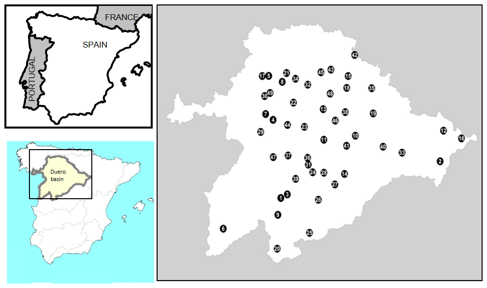
Figure 1Location of study area. The point with the number indicates the location of the agrometeorological stations according to Table 1.
2.1 Description of the study area
The study focuses on the Spanish part of the Duero hydrographic basin. The international hydrographic Duero basin is the most extensive of the Iberian Peninsula; with an area 98 073 km2, it includes the territory of the Duero River basin as well as the transitional waters of the Porto estuary and the associated Atlantic coastal waters (CHD, 2019). It is a shared territory between Portugal, with 19 214 km2 (19.6 % of the total area), and Spain, with 78 859 km2 (80.4 % of the total area). The Duero River basin is located in Spain, between 43∘5′ and 40∘10′ N and 7∘4′ and 1∘50′ W (Fig. 1). This basin aligns almost exactly with the so-called Submeseta Norte, an area with an average altitude of 700 m, delimited by mountain ranges with a much drier central zone that contains large aquifers, which is the most important area of agricultural production; 98.4 % of the Duero basin belongs to the autonomous community of Castilla and Léon, and 70 % of the average annual precipitation is used directly by the vegetation or evaporated from surface – this represents 35 000 h m3. The remaining (30 %) is the total natural runoff. The Mediterranean climate is the predominant climate; 90 % of the surface is affected by summer drought conditions. The average annual values are a temperature of 12 ∘C and precipitation of 612 mm. However, precipitation ranges from minimum values of 400 mm (south–central area of the basin) to a maximum of 1800 mm in the northeast of the basin (CHD, 2019). According to Lautensach (1967), 30 mm is the threshold definition of a dry month. Therefore, between two and five dry periods can be found in the basin (Ceballos et al., 2004). Moreover, the climate variability, especially precipitation, exhibited in the last decade has decreased the water availability for irrigation in this basin (Segovia-Cardozo et al., 2019).
The Duero basin has 4×10⁶ ha of rainfed crops and some 500 000 ha of irrigated crops that consume 75 % of the basin's water resources. Barley (Hordeum vulgare L.) is the most important rainfed crop in the basin, occupying 36 % of the national crop surface, followed by wheat (Triticum aestivum L.), with 30 % (MAPAMA, 2019). Sunflower (Helianthus annuus L.) represents 30 % of the national crop surface. This crop is mainly unirrigated (90 %). Maize (Zea mays L.), alfalfa (Medicago sativa L.) and sugar beet (Beta vulgaris L. var. sacharifera) are the main irrigated crops. These crops represents 29 %, 30 % and 68 % of the national crop area, respectively. Finally, vines (Vitis vinifera L.) fill 72 000 ha, being less than 10 % irrigated. For the irrigated crops of the basin there are water allocations that fluctuate depending on the availability of water during the agricultural year and the type of crop. These values fluctuate from 1200–1400 m3 ha−1 for vines to 6400–7000 m3 ha−1 for maize and alfalfa. The use rates of the irrigation systems used in the basin are as follows: 25 %, 68 % and 7 % for surface, sprinkler and drip irrigation, respectively (Plan Hidrológico, 2019).
2.2 Meteorological data
The daily climate data were downloaded from 49 stations (Fig. 1b) from the agrometeorological network SIAR (Agroclimatic Information System for Irrigation; SIAR in Spanish), which is managed by the Spanish Ministry of Agriculture, Fisheries and Food (SIAR, 2018), providing the basic meteorological data from weather stations distributed throughout the Duero basin (Table 1). Each station incorporates measurements of air temperature (T) and relative humidity (RH; Vaisala HMP155), precipitation (ARG100 rain gauge), solar global radiation (pyranometer Skye SP1110), and wind direction and wind speed (u; wind vane and R.M. Young 05103 anemometer). Sensors were periodically maintained and calibrated, and all data were recorded and averaged hourly on a data logger (Campbell CR10X and CR1000). Characteristics of the agrometeorological stations were described by (Moratiel et al., 2011, 2013a). For quality control, all parameters were checked, and the sensors were periodically maintained and calibrated, with all data being recorded and averaged hourly on a data logger. The database calibration and maintenance are carried out by the Ministry of Agriculture. Transfer of data from stations to the main center is accomplished by modems; the main center incorporates a server which sequentially connects to each station to download the information collected during the day. Once the data from the stations are downloaded, they are processed and transferred to a database. The main center is responsible for quality control procedures that comprise the routine maintenance program of the network, including sensor calibration, checking for validity values and data validation. Moreover, the database was analyzed to find incorrect or missing values. To ensure that high-quality data were used, we used quality control procedures to identify erroneous and suspect data. The quality control procedures applied are the range and limit test, step test, and internal consistency test (Estevez et al., 2016).
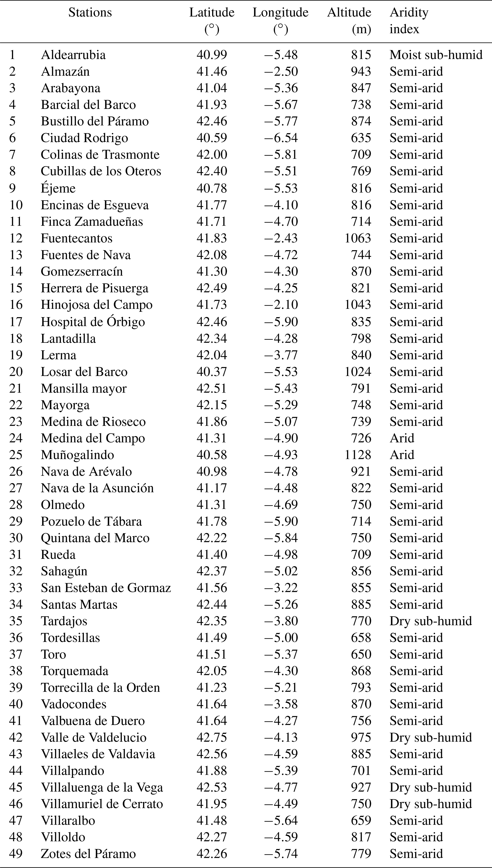
The period studied was from 2000 to 2018, although the start date may fluctuate depending on the availability of data. Table 1 shows the coordinates of the agrometeorological stations used in the Duero basin and the aridity index based on UNEP (1997). Table 1 shows the predominance of the semi-arid climate zone, with 42 stations of the 49 being semi-arid, 2 being arid, 4 being dry sub-humid and 1 being moist sub-humid.
2.3 Estimates of reference evapotranspiration
2.3.1 FAO Penman–Monteith (FAO PM)
The FAO recommends the PM method for computing ETo and evaluating other ETo models like the Penman–Monteith model using only temperature data (PMT) and other temperature-based models (Allen et al., 1998). The method estimates the potential evapotranspiration from a hypothetical crop with an assumed height of 0.12 m, having an aerodynamic resistance of (ra) 208∕u2 (u2 is the mean daily wind speed measured at a 2 m height over the grass), a surface resistance (rs) of 70 s m−1 and an albedo of 0.23, closely resembling the evaporation of an extension surface of green grass with a uniform height that is actively growing and adequately watered. The ETo (mm d−1) was estimated following FAO 56 (Allen et al., 1998):
In Eq. (1), Rn is net radiation at the surface (MJ m−2 d−1), G is ground heat flux density (MJ m−2 d−1), γ is the psychrometric constant (kPa ∘C−1), T is mean daily air temperature at 2 m height (∘C), u2 is wind speed at 2 m height (m s−1), es is the saturation vapor pressure (kPa), ea is the actual vapor pressure (kPa) and Δ is the slope of the saturation vapor pressure curve (kPa ∘C−1). According to Allen et al. (1998) in Eq. (1), G can be considered to be zero.
Table 1Agrometeorological station used in the study. Coordinates and aridity index are shown.
2.3.2 Hargreaves–Samani (HS)
The scarcity of available agrometeorological data (mainly global solar radiation, air humidity and wind speed) limit the use of the FAO PM method in many locations. Allen et al. (1998) recommended applying the Hargreaves–Samani expression in situations where only the air temperature is available. The HS formulation is an empirical method that requires empirical coefficients for calibration (Hargreaves and Samani, 1982, 1985). The Hargreaves–Samani (Hargreaves and Samani, 1982, 1985) method is given by the following equation:
where ETo is the reference evapotranspiration (mm d−1); Ho is extraterrestrial radiation (MJ m−2 d−1); kRS is the Hargreaves empirical coefficient; and Tm, Tx and Tn are the daily mean, maximum air temperature and minimum air temperature (∘C), respectively. The value kRS was initially set to 0.17 for arid and semi-arid regions (Hargreaves and Samani, 1985). Hargreaves (1994) later recommended using the value of 0.16 for interior regions and 0.19 for coastal regions. Daily temperature variations can occur due to other factors such as topography, vegetation, humidity, etc.; thus using a fixed coefficient may lead to errors. In this study, we use 0.17 as the original coefficient (HSO) and the calibrated coefficient kRS (HSC). kRS reduces the inaccuracy, thus improving the estimation of ETo. This calibration was done for each station.
2.3.3 Penman–Monteith temperature (PMT)
The FAO PM, when applied using only measured temperature data, is referred to as PMT and retains many of the dynamics of the full-data FAO PM (Pereira et al., 2015; Hargreaves and Allen, 2003). Humidity and solar radiation are estimated in the PMT model using only air temperature as input for the calculation of ETo. Wind speed in the PMT model is set to the constant value of 2 m s−1 (Allen et al., 1998). In this model, where global solar radiation (or sunshine data) is lacking, the difference between the maximum and minimum temperature can be used, as an indicator of cloudiness and atmospheric transmittance, for the estimation of solar radiation (Eq. 3; Hargreaves and Samani, 1982). Net solar shortwave and longwave radiation estimates are obtained as indicated by Allen et al. (1998), in Eqs. (4) and (5), respectively. The expression of PMT is obtained as indicated in the following:
where Rs is solar radiation (MJ m−2 d−1); Rns is net solar shortwave radiation (MJ m−2 d−1); Ho is extraterrestrial radiation (MJ m−2 d−1); and Ho was computed as a function of site latitude, solar angle and the day of the year (Allen et al., 1998). Tx is the daily maximum air temperature (∘C), and Tn is the daily minimum air temperature (∘C). For kRS Hargreaves (1994) recommended using kRS=0.16 for interior regions and kRS=0.19 for coastal regions. For better accuracy the coefficient kRS can be adjusted locally (Hargreaves and Allen, 2003). In this study two assumptions of kRS were made: one where a value of 0.17 was fixed and another where it was calibrated for each station,
where Rnl is net longwave radiation (MJ m−2 d−1), Tx is daily maximum air temperature (∘C), Tn is daily minimum air temperature (∘C), Td is dew point temperature (∘C) calculated with the Tn according to Todorovic et al. (2013), σ is the Stefan–Boltzmann constant for a day ( MJ K−4 m−2 d−1) and z is the altitude (m):
where PMT is the reference evapotranspiration estimate by the Penman–Monteith temperature method (mm d−1), PMTrad is the radiative component of PMT (mm d1), PMTaero is the aerodynamic component of PMT (mm d−1), Δ is the slope of the saturation vapor pressure curve (kPa ∘C−1), γ is the psychrometric constant (kPa ∘C−1), Rns is net solar shortwave radiation (MJ m−2 d−1), Rnl is net longwave radiation (MJ m−2 d−1), G is ground heat flux density (MJ m−2 d−1), considered to be zero according to Allen et al. (1998), Tm is mean daily air temperature (∘C), Tx is maximum daily air temperature, Tn is mean daily air temperature, Td is dew point temperature (∘C) calculated with the Tn according to Todorovic et al. (2013), u2 is wind speed at 2 m height (m s−1) and es is the saturation vapor pressure (kPa). In this model two assumptions of kRS were made: one where a value of 0.17 was fixed and another where it was calibrated for each station.
2.3.4 Calibration and models
We studied two methods to estimate the ETo: the HS method and the reference evapotranspiration estimate by PMT. Within these methods, different adjustments are proposed based on the adjustment coefficients of the methods and the missing data. The parametric calibration for the 49 stations was applied in this study. In order to decrease the errors of the evapotranspiration estimates, local calibration was used. The seven methods used with the coefficient (kRS) of the calibrated and characteristics in the different locations studied are shown in Table 2. The calibration of the model coefficients was achieved by the nonlinear least-squares fitting technique. The analysis was made on a yearly and seasonal basis. The seasons were the following: (1) winter (December, January and February, or DJF), (2) spring (March, April and May, or MAM), (3) summer (June, July and August, or JJA) and (4) autumn (September, October and November, or SON).
Table 2Characteristics of the models used in this study.
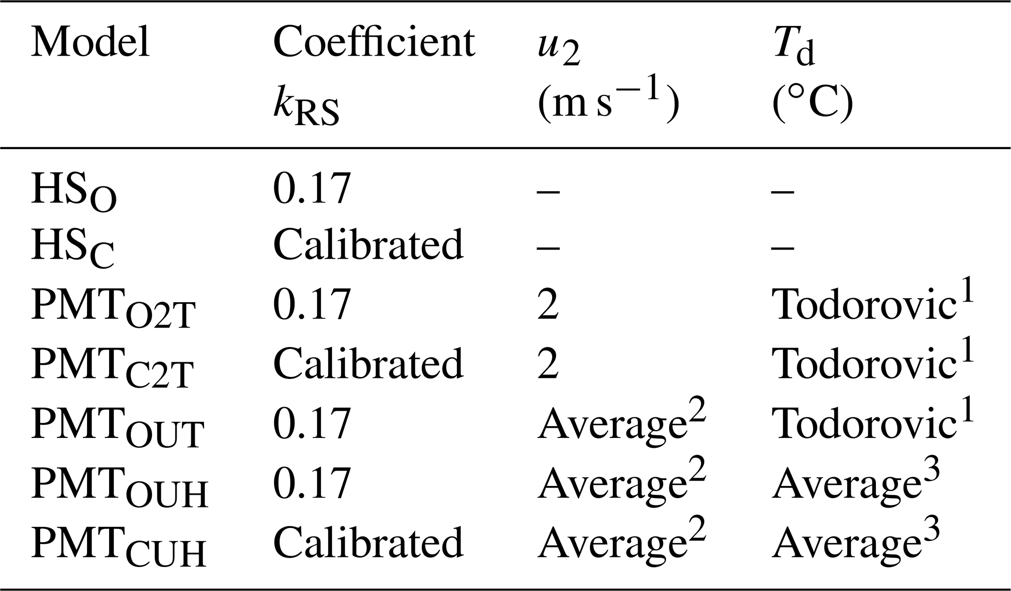
1 Dew point temperature obtained according to Todorovic et al. (2013). 2 Average monthly value of wind speed. 3 Average monthly value of maximum and minimum relative humidity.
2.4 Performance assessment
The model's suitability, accuracy and performance were evaluated using the coefficient of determination (R2; Eq. 9) of the n pairs of observed (Oi) and predicted (Pi) values. Also, the mean absolute error (MAE; mm d−1; Eq. 10), root-mean-square error (RMSE; Eq. 11) and the Nash–Sutcliffe model efficiency (NSE; Eq. 12; Nash and Sutcliffe, 1970) coefficient were used. The coefficient-of-regression line (b), forced through the origin, is obtained by predicted values divided by observed values (ETmodel∕ETFAO56).
The results were represented in a map applying the Kriging method with the Surfer® 8 program:
In the study period the data indicated that the Duero basin is characterized by being a semi-arid climate zone (94 % of the stations), where the P∕ETo ratio is between 0.2 and 0.5 (Todorovic et al., 2013). The mean annual rainfall is 428 mm, while the average annual ETo for Duero basin is 1079 mm, reaching the maximum values in the center–south zone, with values that slightly surpass 1200 mm (Fig. 2). The great temporal heterogeneity is observed in the Duero basin, with values of 7 % of the ETo during the winter months (DJF), while during the summer months (JJA) they represent 47 % of the annual ETo. In addition, the months from May to September represent 68 % of the annual ETo, with similar values to those reported by Moratiel et al. (2011).
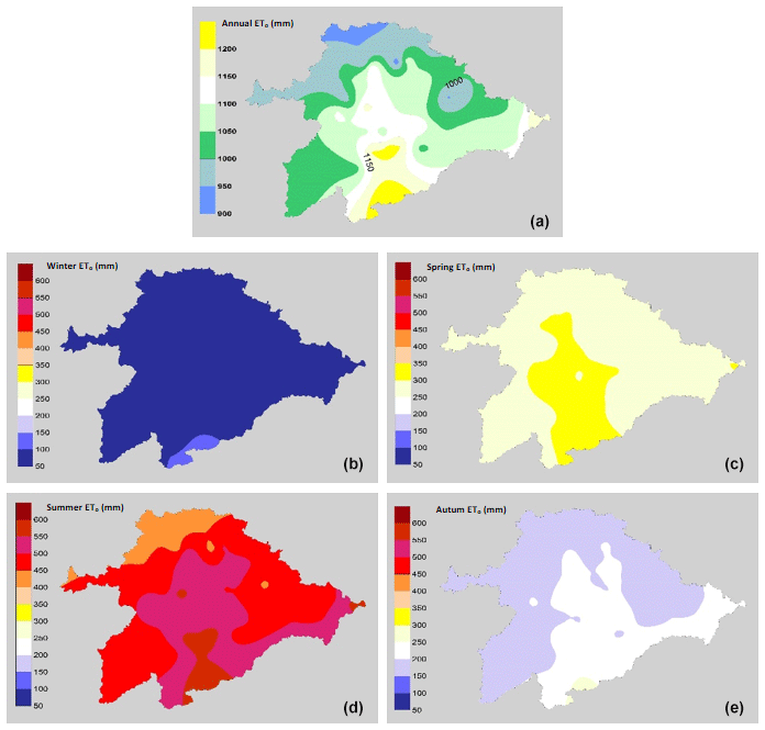
Figure 2Mean values season of ETo (mm) during the study period 2000–2018. (a) Annual, (b) winter (December, January and February, or DJF), (c) spring (March, April and May, or MAM), (d) summer (June, July and August, or JJA) and (e) autumn (September, October and November, or SON).
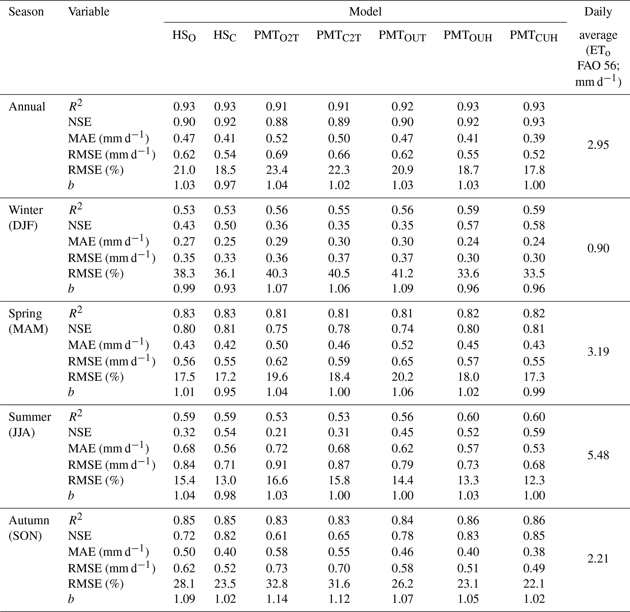
Table 3 shows the different statistics analyzed in the seven models studied as a function of the season of the year and annually. From an annual point of view all models show R2 values higher than 0.91, an NSE higher than 0.88, a MAE less than 0.52, a RMSE lower than 0.69, and underestimates or overestimates of the models by ±4 %. The best behavior is shown by the PMTCHU model, with a MAE and RMSE of 0.39 and 0.52 mm d−1, respectively. PMTCUH shows no tendency to overestimate or underestimate the values in which a coefficient of regression b of 1.0 is observed. This model shows values of the NSE and R2 of 0.93. The models HSC and PMTOUH have similar behavior, with the same MAE (0.41 mm d−1), NSE (0.92) and R2 (0.91). The RMSE is 0.55 mm d−1 for the PMTOUH model and 0.54 mm d−1 for the HSC model. The models PMTOUT and HSO showed slightly better performance than PMTO2T and PMTC2T, given that the last two models showed the worst behavior (Fig. 3). The performance of the models (PMTO2T, PMTOUT and PMTOUH) improves as the averages of wind speed (u) and dew temperature (Td) values are incorporated. The same pattern is shown between the PMTCUH models, where the mean u values and Td are incorporated, and PMTC2T, where u is 2 m s−1 and dew temperature is calculated with the approximation of Todorovic et al. (2013). These adjustments are supported because the adiabatic component of evapotranspiration in the PMT equation is very influential in the Mediterranean climate, especially wind speed (Moratiel et al., 2010).
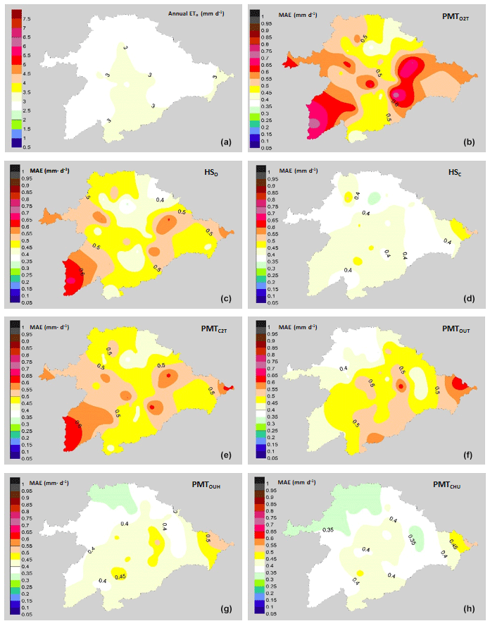
Figure 3Performance of the models with an annual focus. (a) Average annual values of ETo (mm d−1). Mean values of MAE (mm d−1): (b) PMTO2T model, (c) HO model, (d) HC model, (e) PMTC2T model, (f) PMTOUT model, (g) PMTOUH model and (h) PMTCUH model.

Figure 4Performance of the models with a winter focus (December, January and February). (a) Average values of ETo (mm d−1) in winter. Mean values of MAE (mm d−1): (b) PMTO2T model, (c) HO model, (d) HC model, (e) PMTC2T model, (f) PMTOUT model, (g) PMTOUH model and (h) PMTCUH model.
Table 3Statistical indicators for ETo estimation in the seven models studied for different seasons. Average data for the 49 stations studied.
From a spatial perspective, it is observed in Fig. 3 that the areas where the values of the MAE are higher are to the east and southwest of the basin. This is due to the fact that the average wind speed in the eastern zone is higher than 2.5 m s−1; for example, the Hinojosa del Campo station shows average annual values of 3.5 m s−1. The southwestern area shows values of wind speeds below 1.5 m s−1, such as at the Ciudad Rodrigo station, with annual average values of 1.19 m s−1.
These MAE differences are more pronounced in the models in which the average wind speed is not taken, such as the PMTC2T and PMTO2T models. Most of the basin has values of wind speeds between 1.5 and 2.5 m s−1. The lower MAE values in the northern zone of the basin are due to the lower average values of the VPD than the central area, with values of 0.7 kPa in the northern zone and 0.95 kPa in the central zone. The same trends in the effect of wind on the ETo estimates were detected by Nouri and Homaee (2018), who indicated that values outside the range of 1.5–2.5 m s−1 in models where the default u was set at 2 m s−1 increased the error of the ETo. Even for models such as HS, where the influence of the wind speed values is not directly indicated outside of the ranges previously mentioned, their performance is not good, and some authors have proposed HS calibrations based on wind speeds in Spanish basins such as the Ebro Basin (Martínez-Cob and Tejero-Juste, 2004). In our study, the HSC model showed good performance, with MAE values similar to PMTCUH and PMTOUH (Fig. 3). The performance of the models by season of the year changes considerably, obtaining lower adjustments, with values of R2=0.53 for winter (DJF) in the models HSO and HSC and for summer (JJA) in the models PMTO2T and PMTC2T. All models during spring and autumn show R2 values above 0.8. The NSE for models HSO, PMTC2T, PMTO2T and PMTOUT in summer and winter is at unsatisfactory values below 0.5 (Moriasi et al., 2007). The mean values (49 stations) of the MAE (Fig. 4) and RMSE for the models in the winter were 0.24–0.30 and 0.3–0.37 mm d−1, respectively. For spring, the ranges were between 0.42 and 0.52 mm d−1 for the MAE (Fig. 5) and 0.55 and 0.65 mm d−1 for RMSE. In summer, the MAE (Fig. 6) fluctuated between 0.53 and 0.72 mm d−1, and the RMSE fluctuated between 0.68 and 0.91 mm d−1. Finally, in autumn, the values of the MAE (Fig. 7) and RMSE were 0.38–0.58 and 0.49–0.70 mm d−1, respectively (Table 3).

Figure 5Performance of the models with a spring focus (March, April and May). (a) Average annual values of ETo (mm d−1) in spring. Mean values of MAE (mm d−1): (b) PMTO2T model, (c) HO model, (d) HC model, (e) PMTC2T model, (f) PMTOUT model, (g) PMTOUH model and (h) PMTCUH model.

Figure 6Performance of the models with a summer focus (June, July and August). (a) Average values of ETo (mm d−1) in summer. Mean values of MAE (mm d−1): (b) PMTO2T model, (c) HO model, (d) HC model, (e) PMTC2T model, (f) PMTOUT model, (g) PMTOUH model and (h) PMTCUH model.

Figure 7Performance of the models with an autumn focus (September, October and November). (a) Average values of ETo (mm d−1) in autumn. Mean values of MAE (mm d−1): (b) PMTO2T model, (c) HO model, (d) HC model, (e) PMTC2T model, (f) PMTOUT model, (g) PMTOUH model and (h) PMTCUH model.
The model that shows the best performance independently of the season is PMTCUH. The models that can be considered in a second level are HSC and PMTOUH. During the months of more solar radiation (summer and spring) the performance of the HSC model is slightly better than the PMTOUH model. The HSO, PMTO2T, PMTC2T and PMTOUT models have a much poorer performance than the previous models (PMTOUH and HSC). The model that has the worst performance is PMTO2T.
The northern area of the basin is the area in which a lower MAE shows in most models and for all seasons. This is due in part to the fact that the lower values of ETo (mm d−1) are located in the northern zone. On the other hand, the eastern zone of the basin shows the highest values of the MAE due to the strong winds that are located in that area.
During the winter the seven models tested show no great differences between them, although PMTCUH is the model with the best performance. It is important to indicate that during this season the RMSE (%) is placed in all the models above 30 %, so they can be considered to be very weak models. According to Jamieson et al. (1991) and Bannayan and Hoogenboom (2009) the model is considered excellent with a normalized RMSE (%) less than 10 %, good if the normalized RMSE (%) is greater than 10 and less than 20 %, fair if the normalized RMSE (%) is greater than 20 % and less than 30 %, and poor if the normalized RMSE (%) is greater than 30 %. All models that are made during the spring season (MAM) can be considered to be good or fair, since their RMSE (%) fluctuates between 17 % and 20 %. The seven models that are made during summer season (JJA) can be considered to be good, since their RMSE varies from 12 % to 16 %. Finally, the models that are made during autumn (SON) are considered to be fair or poor, fluctuating between 22 % and 32 %. The models that reached values greater than 30 % during autumn were PMTC2T (31 %) and PMTO2T (32 %), which also had a clear tendency to overestimate (Table 3). In the use of temperature models for estimating ETo, it is necessary to know the objective that is set. For the management of irrigation in crops, it is better to test the models in the period in which the species require the contribution of additional water. In many cases, applying the models with an annual perspective with good performance can lead to more accentuated errors in the period of greater water needs. The studies of different temporal and spatial scales of the temperature models for ETo estimation can give valuable information that allows for managing the water planning in zones where the economic development does not allow the implementation of agrometeorological stations due to its high cost.
In annual seasons our data of the RMSE fluctuate from 0.69 mm d−1 (PMTO2T) to 0.52 mm d−1 (PMTO2T). These data are in accordance with the values cited by other authors in the same climatic zone. Jabloun and Sahli (2008) cited a RMSE of 0.41–0.80 mm d−1 for Tunisia. The authors showed the PMT model performance to be better than that for the Hargreaves non-calibrated model. Raziei and Pereira (2013) reported data of the RMSE for a semi-arid zone in Iran to be between 0.27 and 0.81 mm d−1 for the HSC model and 0.30 and 0.79 mm d−1 for PMTC2T, although these authors use monthly averages in their models. Ren et al. (2016) reported values of RMSE to be in the range of 0.51 to 0.90 mm d−1 for PMTC2T and in the range of 0.81 to 0.94 mm d−1 for HSC in semi-arid locations in Inner Mongolia (China). Todorovic et al. (2013) found the PMTO2T method to have better performance than the uncalibrated HS method (HSO), with a RMSE average of 0.47 mm d−1 for PMTO2T and 0.52 HSO. At this point, we should highlight that in our study daily-value data were used.
The original Hargreaves equation was developed by regressing cool-season grass ET in Davis, California; the kRS coefficient is a calibration coefficient. The aridity index for Davis is semi-arid (; Hargreaves and Allen, 2003; Moratiel et al., 2013b), like 94 % of the stations studied, which explains why the behavior of the HSO model is often very similar to HSC. Even so, the calibration coefficient needs to be adjusted for other climates. Numerous studies in the literature have demonstrated the relevance of the kRS calibration model to estimating FAO 56 (Todorovic et al., 2013; Raziei and Pereira, 2013; Paredes et al., 2018).
PMT models have improved, considering the average wind speed. In addition, trends and fluctuations of u have been reported as the factor that most influences ETo trends (Nouri et al., 2017; McVicar et al., 2012; Moratiel et al., 2011). Numerous authors have recommended including, as much as possible, average data of local wind speeds for the improvement of the models, like Nouri and Homaee (2018) and Raziei and Pereira (2013) in Iran, Paredes et al. (2018) in the Azores (Portugal), Djaman et al. (2017) in Uganda, Rojas and Sheffield (2013) in Louisiana (USA), Jabloun and Shali (2008) in Tunisia, and Martinez-Cob and Tejero-Juste (2004) in Spain, among others. In addition, even ETo prediction models based on PMT focus their behavior based on the wind speed variable (Yang et al., 2019). It is important to note that PMTOUT generally has better performance than PMTC2T except for in spring. The difference between both models is that in PMTC2T, kRS is calibrated with wind speed set to 2 m s−1, and in PMTOUT, kRS is not calibrated and has an average wind speed. In this case the wind speed variable has less of an effect than the calibration of kRS, since the average values of wind during spring (2.3 m s−1) are very close to 2 m s−1 and there is no great variation between both settings. In this way, kRS calibration shows a greater contribution than the average of the wind speed to improve the model (Fig. 5e and f). In addition, although u is not directly considered for HS, this model is more robust in regions with speed averages around 2 m s−1 (Allen et al., 1998; Nouri and Homaee, 2018). On the other hand errors in the estimation of relative humidity cause substantial changes in the estimation of ETo, as reported by Nouri and Homaee (2018) and Landeras et al. (2008).
The results of RMSE values (%) of the different models change considerably by season; values are between 16.6 % and 12.3 % for summer and between 41.2 % and 33.5 % for winter. Similar results were obtained in Iran by Nouri and Homaee (2018), where in the months of December–January and February the performance of the PMT and HS models tested had RMSE (%) values above 30 %. Very few studies, as far as we know, have been carried out with adjustments of evapotranspiration models from a temporal point of view, and generally the models are calibrated and adjusted from an annual point of view. Some authors, such as Aguilar and Polo (2011), differentiate seasons between wet and dry, and others, such as Paredes et al. (2018), divide them into summer and winter; Vangelis et al. (2013) take two periods into account, and Nouri and Homaee (2018) do it from a monthly point of view. In most cases, the results obtained in these studies are not comparable with those presented in this study, since the timescales are different. However, it can be noted that the results of the models according to the timescale season differ greatly with respect to the annual scale.
The performance of seven temperature-based models (PMT and HS) was evaluated in the Duero basin (Spain) for a total of 49 agrometeorological stations. Our studies revealed that the models tested on an annual or seasonal basis provide different performance. The values of R2 are higher when they are performed annually, with values between 0.91 and 0.93 for the seven models, but when performed from a seasonal perspective, there are values that fluctuate between 0.5 and 0.6 for summer or winter and 0.86 and 0.81 for spring and autumn. The NSE values are high for models tested from an annual perspective, but for the seasons of spring and summer they are below 0.5 for the models HSO, PMTO2T, PMTC2T and PMTOUT. The fluctuations between models with an annual perspective of the RMSE and MAE were greater than if those models were compared from a seasonal perspective. During the winter none of the models showed good performance, with values of R2>0.59, NSE > 0.58 and RMSE (%) > 30 %. From a practical point of view, in the management of irrigated crops, winter is a season where crop water needs are minimal, with daily average values of ETo around 1 mm due to low temperatures, radiation and VPD. The model that showed the best performance was PMTCUH, followed by PMTOUH and HSC for annual and seasonal criteria. PMTOUH is slightly less robust than PMTCUH during the maximum radiation periods of spring and summer, since PMTCHU performs the kRS calibration. The performance of the HSC model is better in the spring period, which is similar to PMTCHU. The spatial distribution of MAEs in the basin shows that it is highly dependent on wind speeds, obtaining greater errors in areas with winds greater than 2.8 m s−1 (east of the basin) and lower than 1.3 m s−1 (south–southwest of the basin). This information of the tested models at different temporal and spatial scales can be very useful for adopting appropriate measures for efficient water management under the limitation of agrometeorological data and under the recent increments of dry periods in this basin. It is necessary to consider that these studies are carried out at a local scale, and in many cases the extrapolation of the results at a global scale is complicated. Future studies should be carried out in this way from a monthly point of view, since there may be high variability within the seasons.
Evapotranspiration and agrometeorological data are from the Agroclimatic Information System for Irrigation (SIAR), belonging to the Ministry of Agriculture, Fisheries and Food. These data are available at http://eportal.mapa.gob.es/websiar/Inicio.aspx (last access: 2 June 2018). The processing workflow for these data can be seen in Sect. 2 of this paper.
RM and JA developed the idea for the research and methodology and prepared the draft of the paper. RB and AS obtained and processed the raw data. AMT and RM prepared the maps and analyzed the statistical variables obtained. RM, JA, AS and AMT reviewed and edited the paper and contributed to the final paper.
The authors declare that they have no conflict of interest.
This article is part of the special issue “Remote sensing, modelling-based hazard and risk assessment, and management of agro-forested ecosystems”. It is not associated with a conference.
Special thanks are due to the Centro de Estudios e Investigación para la Gestión de Riesgos Agrarios y Medioambientales (CEIGRAM). Also, we would like to acknowledge the referees and especially the editor for their valuable comments and efforts in reviewing and handing our paper.
This research has been supported by MINECO (Ministerio de Economía y Competitividad) through the projects PRECISOST (AGL2016-77282-C3-2-R) and AGRISOST-CM (S2018/BAA-4330).
This paper was edited by Jonathan Rizzi and reviewed by Victor Quej, Pankaj Pandey, and two anonymous referees.
Aguilar, C. and Polo, M. J.: Generating reference evapotranspiration surfaces from the Hargreaves equation at watershed scale, Hydrol. Earth Syst. Sci., 15, 2495–2508, https://doi.org/10.5194/hess-15-2495-2011, 2011.
Allen, R. G.: Evaluation of procedures for estimating grass reference evapotranspiration using air temperature data only, Report submitted to Water Resources Development and Management Service, Land and Water Development Division, United Nations Food and Agriculture Service, Rome, Italy, 1995.
Allen, R. G., Pereira, L. S., Raes, D., and Smith, M.: Crops evapotranspiration, Guidelines for computing crop requirements, Irrigations and Drainage Paper 56, FAO, Rome, 300 pp., 1998.
Allen, R. G., Pereira, L. S., Howell, T. A., and Jensen, E.: Evapotranspiration information reporting: I. Factors governing measurement accuracy, Agr. Water Manage., 98, 899–920, https://doi.org/10.1016/j.agwat.2010.12.015, 2011.
Almorox, J., Quej, V. H., and Martí, P.: Global performance ranking of temperature-based approaches for evapotranspiration estimation considering Köppen climate classes, J. Hydrol., 528, 514–522, https://doi.org/10.1016/j.jhydrol.2015.06.057, 2015.
Annandale, J., Jovanovic, N., Benade, N., and Allen, R. G.: Software for missing data error analysis of Penman-Monteith reference evapotranspiration, Irrig. Sci., 21, 57–67, https://doi.org/10.1007/s002710100047, 2002.
Bannayan, M. and Hoogenboom, G.: Using pattern recognition for estimating cultivar coefficients of a crop simulation model, Field Crop Res., 111, 290–302, https://doi.org/10.1016/j.fcr.2009.01.007, 2009.
Ceballos, A., Martínez-Fernández, J., and Luengo-Ugidos, M. A.: Analysis of rainfall trend and dry periods on a pluviometric gradient representative of Mediterranean climate in Duero Basin, Spain, J. Arid Environ., 58, 215–233, https://doi.org/10.1016/j.jaridenv.2003.07.002, 2004.
CHD: Confederación Hidrográfica del Duero, available at: http://www.chduero.es, last access: 28 January 2019.
Djaman, K., Rudnick, D., Mel, V. C., Mutiibwa, D., Diop, L., Sall, M., Kabenge, I., Bodian, A., Tabari, H., and Irmak, S.: Evaluation of Valiantzas' simplified forms of the FAO-56 Penman-Monteith reference evapotranspiration model in a humid climate, J. Irr. Drain. Eng., 143, 06017005, https://doi.org/10.1061/(ASCE)IR.1943-4774.0001191, 2017.
Droogers, P. and Allen, R. G.: Estimating reference evapotranspiration under inaccurate data conditions, Irrig. Drain. Syst., 16, 33–45, https://doi.org/10.1023/A:1015508322413, 2002.
Estevez, J., García-Marín, A. P., Morábito, J. A., and Cavagnaro, M.: Quality assurance procedures for validating meteorological input variables of reference evapotranspiration in mendoza province (Argentina), Agric. Water Manage., 172, 96–109. https://doi.org/10.1016/j.agwat.2016.04.019, 2016.
Gavilán, P., Lorite, J. I., Tornero, S., and Berengera, J.: Regional calibration of Hargreaves equation for estimating reference ET in a semiarid environment, Agr. Water Manage., 81, 257–281, https://doi.org/10.1016/j.agwat.2005.05.001, 2006.
Hargreaves, G. H.: Simplified coefficients for estimating monthly solar radiation in North America and Europe. Departamental Paper, Dept. of Bio. and Irrig. Engrg., Utah State Univ., Logan, Utah, 1994.
Hargreaves, G. H. and Allen, R. G.: History and Evaluation of Hargreaves Evapotranspiration Equation, J. Irrig. Drain. Eng., 129, 53–63, https://doi.org/10.1061/(ASCE)0733-9437(2003)129:1(53), 2003.
Hargreaves, G. H. and Samani, Z. A.: Estimating potential evapotranspiration, J. Irrig. Drain. Div., 108, 225–230, 1982.
Hargreaves, G. H. and Samani, Z. A.: Reference crop evapotranspiration from ambient air temperature, Microfiche Collect. no. fiche no. 85-2517), Am. Soc. Agric. Eng., USA, 1985.
Jabloun, M. D. and Sahli, A.: Evaluation of FAO-56 methodology for estimating reference evapotranspiration using limited climatic data: Application to Tunisia, Agr. Water Manage., 95, 707–715, https://doi.org/10.1016/j.agwat.2008.01.009, 2008.
Jamieson, P. D., Porter, J. R., and Wilson, D. R.: A test of the computer simulation model ARCWHEAT1 on wheat crops grown in New Zealand, Field Crop Res., 27, 337–350, https://doi.org/10.1016/0378-4290(91)90040-3, 1991.
Landeras, G., Ortiz-Barredo, A., and López, J. J.: Comparison of artificial neural network models and empirical and semi-empirical equations for daily reference evapotranspiration estimation in the Basque Country (Northern Spain), Agr. Water Manage., 95, 553–565, https://doi.org/10.1016/j.agwat.2007.12.011, 2008.
Lautensach, H.: Geografía de España y Portugal, Vicens Vivens, Barcelona, 814 pp., 1967.
López-Moreno, J. I., Hess, T. M., and White, A. S. M.: Estimation of Reference Evapotranspiration in a Mountainous Mediterranean Site Using the Penman-Monteith Equation With Limited Meteorological Data, Pirineos JACA, 164, 7–31, https://doi.org/10.3989/pirineos.2009.v164.27, 2009.
MAPAMA – Ministerio de Agricultura Pesca y Alimentación: Anuario de estadística, available at: https://www.mapa.gob.es/es/estadistica/temas/publicaciones/anuario-de-estadistica/, last access: 28 March 2019.
Martinez, C. J. and Thepadia, M.: Estimating Reference Evapotranspiration with Minimum Data in Florida, J. Irrig. Drain. Eng., 136, 494–501, https://doi.org/10.1061/(ASCE)IR.1943-4774.0000214, 2010.
Martínez-Cob, A. and Tejero-Juste, M.: A wind-based qualitative calibration of the Hargreaves ETo estimation equation in semiarid regions, Agr. Water Manage., 64, 251–264, https://doi.org/10.1016/S0378-3774(03)00199-9, 2004.
McVicar, T. R., Roderick, M. L., Donohue, R. J., Li, L. T., VanNiel, T., Thomas, A., Grieser, J., Jhajharia, D., Himri, Y., Mahowald, N. M., Mescherskaya, A. V., Kruger, A. C., Rehman, S., and Dinpashoh, Y.: Global review and synthesis of trends in observed terrestrial near-surface wind speeds: implications for evaporation, J. Hydrol., 416–417, 182–205, https://doi.org/10.1016/j.jhydrol.2011.10.024, 2012.
Mendicino, G. and Senatore, A.: Regionalization of the Hargreaves Coefficient for the Assessment of Distributed Reference Evapotranspiration in Southern Italy, J. Irrig. Drain. Eng., 139, 349–362, https://doi.org/10.1061/(ASCE)IR.1943-4774.0000547, 2013.
Moratiel, R., Duran, J. M., and Snyder, R.: Responses of reference evapotranspiration to changes in atmospheric humidity and air temperature in Spain, Clim. Res., 44, 27–40, https://doi.org/10.3354/cr00919, 2010.
Moratiel, R., Snyder, R. L., Durán, J. M., and Tarquis, A. M.: Trends in climatic variables and future reference evapotranspiration in Duero valley (Spain), Nat. Hazards Earth Syst. Sci.m 11, 1795–1805, https://doi.org/10.5194/nhess-11-1795-2011, 2011.
Moratiel, R., Martínez-Cob, A., and Latorre, B.: Variation in the estimations of ETo and crop water use due to the sensor accuracy of the meteorological variables, Nat. Hazards Earth Syst. Sci., 13, 1401–1410, https://doi.org/10.5194/nhess-13-1401-2013, 2013a.
Moratiel, R., Spano, D., Nicolosi, P., and Snyder, R. L.: Correcting soil water balance calculations for dew, fog, and light rainfall, Irrig. Sci., 31, 423–429, https://doi.org/10.1007/s00271-011-0320-2, 2013b.
Moriasi, D. N., Arnold, J. G., Van Liew, M. W., Bingner, R. L., Harmel, R. D., and Veith, T. L.: Model evaluation guidelines for systematic quantification of accuracy in watershed simulations, T. ASABE, 50, 885–900, https://doi.org/10.13031/2013.23153, 2007.
Nash, J. E. and Sutcliffe, J. V.: River flow forecasting through conceptual models. Part I – A discussion of principles, J. Hydrol., 10, 282–290, https://doi.org/10.1016/0022-1694(70)90255-6, 1970.
Nouri, M. and Homaee, M.: On modeling reference crop evapotranspiration under lack of reliable data over Iran, J. Hydrol., 566, 705–718, https://doi.org/10.1016/j.jhydrol.2018.09.037, 2018.
Nouri, M., Homaee, M., and Bannayan, M.: Quantitative trend, sensitivity and contribution analyses of reference evapotranspiration in some arid environments underclimate change, Water Resour. Manage., 31, 2207–2224, https://doi.org/10.1007/s11269-017-1638-1, 2017.
Pandey, P. K. and Pandey, V.: Evaluation of temperature-based Penman–Monteith (TPM) model under the humid environment, Model. Earth Syst. Environ., 2, 152, https://doi.org/10.1007/s40808-016-0204-9, 2016.
Pandey, V., Pandey, P. K., and Mahata, P.: Calibration and performance verification of Hargreaves Samani equation in a Humid region, Irrig. Drain., 63, 659–667, https://doi.org/10.1002/ird.1874, 2014.
Paredes, P., Fontes, J. C., Azevedo, E. B., and Pereira, L. S.: Daily reference crop evapotranspiration with reduced data sets in the humid environments of Azores islands using estimates of actual vapor pressure, solar radiation, and wind speed, Theor. Appl. Climatol., 134, 1115–1133, https://doi.org/10.1007/s00704-017-2329-9, 2018.
Pereira, L. S.: Water, Agriculture and Food: Challenges and Issues, Water Resour. Manage., 31, 2985–2999, https://doi.org/10.1007/s11269-017-1664-z, 2017.
Pereira, L. S., Allen, R. G., Smith, M., and Raes, D.: Crop evapotranspiration estimation with FAO56: Past and future, Agr. Water Manage., 147, 4–20, https://doi.org/10.1016/j.agwat.2014.07.031, 2015.
Plan Hidrológico: Plan Hidrológico de la parte española de la demarcación hidrográfica del Duero, 2015–2021, Anejo 5, Demandas de Agua, available at: https://www.chduero.es/web/guest/plan-hidrológico-de-la-parte-española-de-la-demarcación-hidrográfica, last access: 18 February 2019.
Quej, V. H., Almorox, J., Arnaldo, A., and Moratiel, R.: Evaluation of Temperature-Based Methods for the Estimation of Reference Evapotranspiration in the Yucatán Peninsula, Mexico, J. Hydrol. Eng., 24, 05018029, https://doi.org/10.1061/(ASCE)HE.1943-5584.0001747, 2019.
Raziei, T. and Pereira, L. S.: Estimation of ETo with Hargreaves–Samani and FAO-PM temperature methods for a wide range of climates in Iran, Agr. Water Manage., 121, 1–18, https://doi.org/10.1016/j.agwat.2012.12.019, 2013.
Ren, X., Qu, Z., Martins, D. S., Paredes, P., and Pereira, L.S.: Daily Reference Evapotranspiration for Hyper-Arid to Moist Sub-Humid Climates in Inner Mongolia, China: I. Assessing Temperature Methods and Spatial Variability, Water Resour. Manage., 30, 3769–3791, https://doi.org/10.1007/s11269-016-1384-9, 2016.
Rojas, J. P. and Sheffield, R. E.: Evaluation of daily reference evapotranspiration methods as compared with the ASCE-EWRI Penman-Monteith equation using limited weather data in Northeast Louisiana, J. Irrig. Drain. Eng., 139, 285–292, https://doi.org/10.1061/(ASCE)IR.1943-4774.0000523, 2013.
Segovia-Cardozo, D. A., Rodríguez-Sinobas, L., and Zubelzu, S.: Water use efficiency of corn among the irrigation districts across the Duero river basin (Spain): Estimation of local crop coefficients by satellite images, Agr. Water Manage., 212, 241–251, https://doi.org/10.1016/j.agwat.2018.08.042, 2019.
SIAR: Sistema de información Agroclimática para el Regadío, available at: http://eportal.mapama.gob.es/websiar/Inicio.aspx, last access: 2 June 2018.
Todorovic, M., Karic, B., and Pereira, L. S.: Reference Evapotranspiration estimate with limited weather data across a range of Mediterranean climates, J. Hydrol., 481, 166–176, https://doi.org/10.1016/j.jhydrol.2012.12.034, 2013.
Tomas-Burguera, M., Vicente-Serrano, S. M., Grimalt, M., and Beguería, S.: Accuracy of reference evapotranspiration (ETo) estimates under datascarcity scenarios in the Iberian Peninsula, Agr. Water Manage., 182, 103–116, https://doi.org/10.1016/j.agwat.2016.12.013, 2017.
Trajkovic, S.: Temperature-based approaches for estimating reference evapotranspiration, J. Irrig. Drain. Eng., 131, 316–323, https://doi.org/10.1061/(ASCE)0733-9437(2005)131:4(316), 2005.
UNEP: World atlas of desertification, in: 2nd Edn., edited by: Middleton, N. and Thomas, D., Arnold, London, 182 pp., 1997.
Vangelis, H., Tigkas, D., and Tsakiris, G.: The effect of PET method on Reconnaissance Drought Index (RDI) calculation, J. Arid Environ., 88, 130–140, https://doi.org/10.1016/j.jaridenv.2012.07.020, 2013.
Villalobos, F. J., Mateos, L., and Fereres, E.: Irrigation Scheduling Using the Water Balance, in: Principles of Agronomy for Sustainable Agriculture, edited by: Villalobos, F. J. and Fereres, E., Springer International Publishing, Switzerland, 269–279, 2016.
Yang, Y., Cui, Y., Bai, K., Luo, T., Dai, J., and Wang, W.: Shrot-term forecasting of daily refence evapotranspiration using the reduced-set Penman–Monteith model and public weather forecast, Agr. Water Manage., 211, 70–80, https://doi.org/10.1016/j.agwat.2018.09.036, 2019.