the Creative Commons Attribution 4.0 License.
the Creative Commons Attribution 4.0 License.
 | 01 Apr 2020
Exposure of real estate properties to the 2018 Hurricane Florence flooding
Marco Tedesco
Steven McAlpine
Jeremy R. Porter
Quantifying the potential exposure of property to damages associated with storm surges, extreme weather and hurricanes is fundamental to developing frameworks that can be used to conceive and implement mitigation plans as well as support urban development that accounts for such events. In this study, we aim at quantifying the total value and area of properties exposed to the flooding associated with Hurricane Florence that occurred in September 2018. To this aim, we implement an approach for the identification of affected areas by generating a map of the maximum flood extent obtained from a combination of the flood extent produced by the Federal Emergency Management Agency's (FEMA's) water marks with those obtained from spaceborne radar remote-sensing data. The use of radar in the creation of the flood extent allows for those properties commonly missed by FEMA's interpolation methods, especially from pluvial or non-fluvial sources, and can be used in more accurately estimating the exposure and market value of properties to event-specific flooding. Lastly, we study and quantify how the urban development over the past decades in the regions flooded by Hurricane Florence might have impacted the exposure of properties to present-day storms and floods. This approach is conceptually similar to what experts are addressing as the “expanding bull's eye effect”, in which “targets” of geophysical hazards, such as people and their built environments, enlarge as populations grow and spread. Our results indicate that the total value of property exposed to flooding during Hurricane Florence was USD 52 billion (in 2018 USD), with this value increasing from USD ∼10 billion at the beginning of the past century to the final amount based on the expansion of the number of properties exposed. We also found that, despite the decrease in the number of properties built during the decade before Florence, much of the new construction was in proximity to permanent water bodies, hence increasing exposure to flooding. Ultimately, the results of this paper provide a new tool for shedding light on the relationships between urban development in coastal areas and the flooding of those areas, which is estimated to increase in view of projected increasing sea level rise, storm surges and the strength of storms.
- Article
(20933 KB) -
Supplement
(4186 KB) - BibTeX
- EndNote


The projected rise in sea level, increased floods and storm surge, and associated consequences over the 21st century has the potential to do immense economic harm. The economic impact is particularly worrisome in the US because the most valuable real estate, densest communities and most productive economic engines are situated disproportionately in coastal regions (Fu et al., 2016; NOAA, 2013; Kildow et al., 2014). Recent research has highlighted an ongoing economic signal associated with high-probability flooding events and real estate transactions in coastal communities that can be observed with historical data (see McAlpine and Porter, 2018; Keenan et al., 2018; and Bernstein et al., 2019), suggesting that sea level rise (SLR) already produces negative economic consequences on coastal communities. Furthermore, there is abundant evidence indicating that we are only seeing the first signs of a much more problematic issue both in terms of the flooding scale and the magnitude of associated economic losses (see Fu et al., 2016; Hallegatte et al., 2011; Bin et al., 2008, 2011; Parsons and Powell, 2001; Michael, 2007). In this regard, a SLR of ∼2 m (e.g., 6 ft) would flood roughly 100 000 homes only in New York City with a total value of USD 39 billion (note that we use 2018 as a reference for the dollar year throughout this paper unless otherwise mentioned); a 3 m (10 ft) rise would flood 300 000 homes and properties with a total value of almost USD 100 billion (UCSUSA, 2019). The equivalent figures for Miami are 54 000 homes and properties valued at USD 14 billion being at risk with a ∼2 m rise and 130 000 homes and properties valued at USD 32 billion at risk with a ∼3 m rise.
Recent events such as hurricanes Katrina, Irma and Florence have highlighted the issues related to floods and extreme events even more. In particular, Florence was one of the most devastating hurricanes in history, as it combined storm surge, strong winds and extreme precipitation. It began as a tropical storm on 1 September 2018 over the islands of Cabo Verde off the coast of western Africa and peaked as a Category 4 hurricane with winds up to 225 km h−1 before making landfall as a Category 1 hurricane on 14 September 2018 over Wrightsville Beach, North Carolina. By 11:15 UTC on Friday, 14 September 2018, Florence was downgraded to a tropical storm, and early on Sunday, 16 September, it became a tropical depression, with winds of about 360 km h−1. At least 51 people died as a consequence of flooding associated with rain records (up to 3 feet of rain in some areas according to the National Weather Service), with more than 400 000 houses without power and a total damage of USD 24 billion (https://www.ncdc.noaa.gov/billions/events.pdf, last access: October 2019).
The human cost of Hurricane Florence was a reminder of the power of such storms, and these storms are likely becoming more impactful, as their surge reaches further inland due to changing tracks, increased strength and rising seas. The increasing exposure of the public and properties to events similar to Hurricane Florence has unintended consequences of raising the awareness and concern to all types of climate-related events (Borenstien and Fingerhut, 2019). Such is likely the case in much of the recent research on real estate market responses to higher-probability flooding associated with nuisance tidal flooding events (McAlpine and Porter, 2018). In their study, MacAlpine and Porter (2018) found that properties in Miami-Dade County at risk of frequent tidal flooding had lost over USD 430 million in property value relative to homes that were not a risk of repeated tidal flooding events. Likewise, and also centered in the Miami-Dade region, Keenan et al. (2018) found that homes at lower elevations were being penalized on the market relative to homes at higher elevations. Moreover, in another analysis, Bernstein et al. (2019) found a similar penalty for homes at risk of flooding from an increase in the SLR but found that this penalty was primarily driven by investors and uneven access to information associated with risk. All of these studies identify an increase in awareness of SLR-related flooding events, and all document the fact that this trend is relatively new (since about the middle of the last decade). Of particular importance to the recent market response is the fact that increased probability is an important driving force. In the work undertaken by Bernstein et al. (2019), for example, the price penalty for homes at risk of flooding is explicitly driven by the sophistication of investors and their access to risk tools aimed at helping them to make decisions about property value as well as long-term appreciation over time. McAlpine and Porter (2018) also found, in this regard, that risk associated with being impacted by a Category 1 hurricane is correlated with potential loss property value but not the probability of being impacted by a higher-category storm. In each of these cases, the research suggests that the real estate market is becoming more sensitive to the probability of damage associated with inundation from flooding events due to rising seas, storm surges, nuisance flooding and consequences of a changing climate. On the other hand, research out of the University of Pennsylvania's Wharton Risk Center by Kunthreuther et al. (2018) found that the elasticity concerning the housing market tends to show quick recoveries in areas where the experience of climate catastrophes is characterized as a market shock. Market shocks are generally thought of as one-time (or contiguous time period) events that negatively impact the housing market. Due to the nature of market shocks being lower probability and harder to predict, the housing market tends to see them as unlikely and related to collective internalizations associated with myopia, amnesia, optimism, inertia, simplification and herding (Kunthreuther et al., 2018). However, market stressors are ubiquitous, high-probability events that are generally predictable and have historical certainty. In the context in which we are working, increased and unmanageable tidal flooding could be considered a market stressor, while the impact of a single hurricane event could constitute a market shock. Historically, market shocks (such as hurricanes) are much more expensive, in terms of actual economic impacts, and consume more media attention, in terms of the coverage of the events.
Several studies have recently focused on assessing damages from Hurricane Florence. Roberson et al. (2019) use overhead imagery, including synthetic-aperture radar (SAR) and optical data, to study the impact of Florence on livestock wastewater and crop health. Srikanto et al. (2019) study the spatial distribution of fatalities and associated demographics, indicating that 93 % of the affected buildings were residential structures. The proper quantification of the impact of Hurricane Florence (or more in general of extreme events) is helpful not only for addressing the recovery of the communities impacted by the event but also for providing tools to policymakers, urban planners and city managers that will ultimately guide them through the decision process of reducing the impacts of future events. If it is true, indeed, that climate change is and will be influencing the frequency and strength of storms and floods, it is also true that the exposure of anthropogenic structures and lives is a function of urbanization factors such as, for example, the building of new properties in proximity to the coast and to water bodies. In this context, it becomes crucial to understand and quantify how urban development has impacted the exposure of properties and population to present-day storms and floods. For example, one of the most devastating hurricanes over the same region before Florence was Hurricane Hugo, reaching the Carolinas on 10 September 1989, with winds up to 260 km h−1 and a total estimated damage of USD 9.45 billion (in 1989 USD, equivalent to USD 19 billion of 2018 USD) and 60 fatalities. Unlike 1989, we have today improved observational and modeling tools that allow us to better estimate the maximum flood extent, a key parameter needed to estimate the potential exposure to damage of properties and other infrastructures. From a modeling point of view, hydrological and hydrodynamic models, in conjunction with improved digital elevation models and the ingestion of gauge observation or observation of high-water marks, offer the opportunity to generate estimates of maximum flood extent (FEMA, 2019).
We aim at understanding the usefulness of remotely sensed satellite data as a method for the identification of impacted areas and for delineating the maximum flood extent. Specifically, we report results concerning the mapping of the flood extent associated with Hurricane Florence estimated from SAR data and compare such extent with the maximum flood extent provided by the Federal Emergency Management Agency (FEMA). From that exposure, we are able to quantify the property value and total area exposed to Hurricane Florence by combining the flood extent coverage with a database containing publicly available property value attributes. Despite recent studies that have started to focus on the spatio-temporal variability in property values and human settlements in hurricane-prone areas (e.g., Huang et al., 2019) and on the market responses to increases in observed flooding events (e.g., McAlpine and Porter, 2019; Keenan et al., 2018), no study, to our knowledge, has focused on the impact of urban growth on the property exposed to Hurricane Florence. Addressing this point is crucial to account for those impacts related to the choices that our society makes to continue the expansion of urban areas and that have been addressed by experts as the expanding bull's eye effect (Ashley and Strader, 2016), in which targets of geophysical hazards, such as people and their built environments, enlarge as populations grow and spread. The term bull's eye is used here to define the eye or center of a storm. Our approach is complementary to the approaches focusing on the bull's eye effect and to those calculating the impact of floods under future climate scenarios (e.g., sea level rise or storm surge is changing but the property distribution remains the same). Specifically, we assess the potential exposure of properties using a dataset containing, among other information, when each property was built and use that information to estimate the potential exposure of buildings to Hurricane Florence that would have occurred in the past decades.
2.1 Sentinel-1 radar data and identification of inundated areas
From an observational point of view, spaceborne and airborne remote sensing (e.g., Schumann et al., 2011), as well as UAV-based approaches (e.g., Gebrehiwot et al., 2019), offer powerful tools to monitor flood extent (e.g., Domeneghetti et al., 2019; Schumann et al., 2018; Schumann, 2018; Giordan et al., 2018). Optical data can map the presence of surface water at relatively high spatial resolution and accuracy, but it is limited by the presence of clouds (Schumann et al., 2018). On the other hand, datasets collected in the microwave region, such as those collected by synthetic-aperture radar (SAR), are not limited by the presence of clouds (Schumann et al., 2018; Manavalan, 2017; Huang et al., 2018). The recent launch of Sentinel-1 ESA sensors in September 2014 (Sentinel-1A) and April 2016 (Sentinel-1B; https://sentinel.esa.int/web/sentinel/missions/sentinel-1, last access: October 2019) allows mapping of flood extent at unprecedented temporal and spatial resolutions. The combination of the two sensors provides a nominal 6 d repeat cycle over the Equator and 12 d repeat cycle over North America (Torres et al., 2012) at a horizontal spatial resolution of the SAR data of 10 m. For the purpose of this study, we obtained Sentinel-1 data from the National Aeronautics and Space Administration Alaska Satellite Facility (NASA/ASF, https://earthdata.nasa.gov/about/daacs/daac-asf, last access: October 2019). More information on the Sentinel-1 sensors can be found at https://sentinel.esa.int/web/sentinel/missions/sentinel-1 (last access: October 2019). Specific details on the SAR-based approach used in this study are reported in the Supplement.
2.2 FEMA maximum water extent during Florence
We supplement the radar-derived flood extent with FEMA's high-water-mark-based depth grids and inundation polygons from observed and collected Hurricane Florence data. High-water marks (HWMs) are point data collected using high-resolution real-time kinematic (RTK) GPS systems or other methods. HWM points represent the highest extent of riverine flood or coastal storm surge inundation. The raw data are available at the FEMA Natural Hazard Risk Assessment Program (NHRAP) site and were downloaded for all basins available per FEMA's collection efforts following the hurricane event (https://data.femadata.com/FIMA/NHRAP/Florence/, last access: October 2019).
The FEMA maximum water extent is distributed as a GIS raster file created to represent the extent of riverine or coastal storm inundation following larger flooding events. The file is created as a derived product following the creation of the maximum depth grid raster file, which is obtained using FEMA HWM data and FEMA's Digital Flood Insurance Rate Map (DRIRM) Base Flood Elevations (lidar-based elevation data). Using those datasets, a grid is obtained to estimate the height of water at any given point between HWMs based on base elevation. From this, we extracted a secondary file measuring only the extent of inundation from the storm surge. The FEMA dataset is distributed as an ArcGIS® geodatabase (.gdb format), and we rasterized it at a spatial resolution of 10 m to match the spatial resolution of the SAR data. More information on the FEMA approach for estimating maximum flood extent can be found at https://data.femadata.com/FIMA/NHRAP/Florence (last access: October 2019).
2.3 Property database
Property value data are compiled from each individual property's county assessor in the form of the property tax assessed value. The data were obtained from a third-party provider, ATTOM™ Data Solutions, which provides high-quality parcel-level information on all properties in the United States and in a value-added format (https://www.attomdata.com, last access: October 2019). The process by which the data are compiled relies solely on publicly available data and the processing, cleansing and standardizing of that data in order to make it available in a user-friendly format. The data used in this analysis include the property's last-recorded assessment value for all properties within the states of North and South Carolina as well as the year when the property was built. Each county's assessment process varies, and, as such, the data are subject to known potential limitations associated with the timing and frequency of home assessments undertaken by local county officials in which the property is located. However, the data also give us the best available comprehensive look at tax base value in a geolocated format for comparison to our storm surge coverage file.
3.1 Assessment of remote-sensing-derived areas vs. FEMA maximum water extent
Inundated areas (including permanent water bodies) obtained from Sentinel-1 data and FEMA are reported, respectively, as blue (radar) and red (FEMA) regions in Fig. 1. We used a total of 12 Sentinel-1 images collected between 14 and 19 September 2018 and whose footprints are shown in the inset in the top left corner of Fig. 1. Specific names and acquisition times of the radar images are reported in the Supplement. We used the 12 images in order to maximize the covered area and to account for the temporal evolution of surface water after the landfall of Hurricane Florence associated with heavy, persistent rainfall.
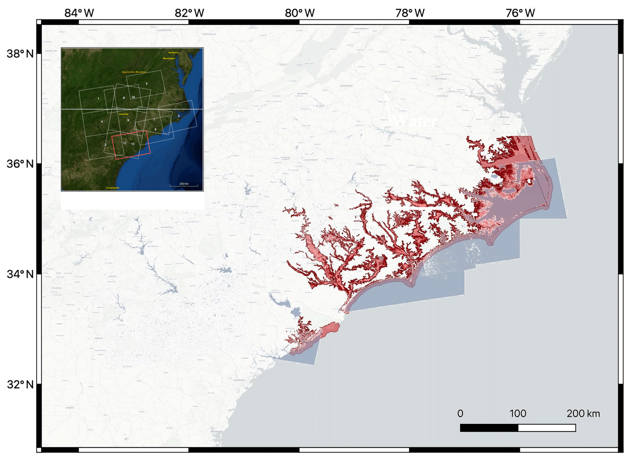
Figure 1Map of inundated areas estimated by FEMA (red) and by the Sentinel-1 radar images (blue). The inset in the top left corner shows the footprint of the several radar images to create the composite water extent map. Acquisition times and other details concerning the radar images are available in the Supplement.
The comparison between the maximum water extent estimated by FEMA and the water extent mask obtained from Sentinel-1 indicates a matching score (defined here as the percentage of flooded pixels identified by Sentinel-1 with respect to the total number of flooded pixels identified by FEMA) of 11.3 % and a commission error (defined as the relative percentage of pixels when Sentinel-1 detects flooded areas but FEMA does not with respect to the total number of FEMA flooded pixels) of 9.2 %. We note here that the FEMA map is based on a combination of modeled and measured quantities and might miss flooding associated with heavy rains, as in the case of Hurricane Florence. Consequently, it is possible that some areas that were flooded according to the radar images were not included in the FEMA maps. As an example, Fig. 2 shows the maximum water extent from FEMA (red) together with the one derived from Sentinel-1 data (blue) nearby the town of Bennettsville, South Carolina (34.6174∘ N, 79.6848∘ W). Areas in green show the location of the properties within our database. We note that the radar sensor detects water over agricultural fields that are not marked by the FEMA maps as flooded, showing a potential improvement over the FEMA maps. Our analysis of the Sentinel-1 backscattering coefficients (not shown here) indicates that the backscattering values recorded for the regions where flooding was identified by the radar were relatively low (e.g., well below the threshold value and on the order of dB or below), indicating that those were, indeed, inundated areas.
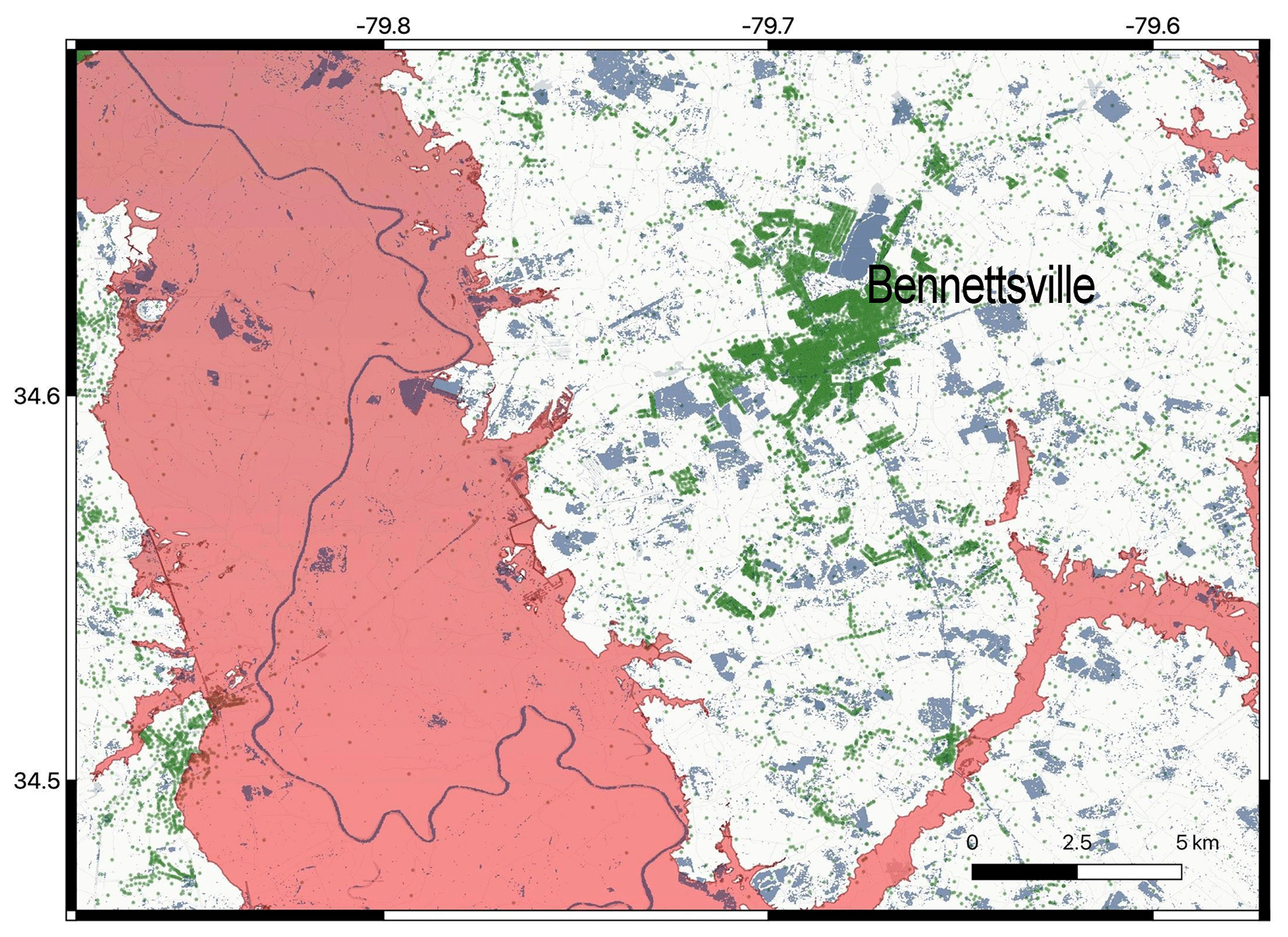
Figure 2Map of inundated areas estimated by FEMA (red) and by Sentinel-1 (blue) near the town of Bennettsville, South Carolina (34.6174∘ N, 79.6848∘ W). Green areas represent the locations of properties for this area.

Figure 3Time series of (a) tide gauge mean sea level (m.s.l.) height (m) recorded at Wrightsville Beach, North Carolina, and (b) daily discharge (cubic meters per hour) and (c) daily gauge height (meters) recorded at Lumber River (USGS gauge 02134170), North Carolina, between 1 and 30 September 2018. In (a) blue line refers to predictions, whereas green lines refer to verified values. In (a) data and plot were obtained from https://tidesandcurrents.noaa.gov/ (last access: October 2019). For data plotted in (b) and (c) we obtained data and graphs from https://waterdata.usgs.gov/ (last access: October 2019). In (a) and (c) we also report, as dashed vertical lines, the acquisition times of the available Sentinel-1 data.
Another factor complicating the comparison between Sentinel-1 and FEMA inundated regions regards the acquisition time of the radar images, which are collected before or after the time of the maximum water extent. Figure 3a shows the time series of the water height (mean sea level in meters) for the ocean tide gauge located in Wrightsville Beach, North Carolina (ID no. 8658163), where Hurricane Florence made landfall. Maximum water height was reached on the same day at around 15:00 UTC. The image also shows the acquisition time of the Sentinel-1B (14 September 2018, 11:15:05 UTC) and Sentinel-1A (14 September 2018, 23:05:48 UTC) as vertical, dashed lines, indicating that such images were, indeed, acquired before and after the time when the water reached the maximum extent. River gauge data also show that, because of the heavy precipitation, the maximum water discharge and gauge heights inland occurred a few days after Hurricane Florence made landfall. In this regard, Fig. 3b and c show, respectively, the daily discharge (in m3 h−1) and daily gauge height (in m) recorded at the river gauge station of Lumberton, North Carolina (34.6182∘ N, 79.0086∘ W), located about 150 km inland. The data show the peak discharge and water heights late in the evening of 17 September 2018. For this same area the radar data were collected when the tide gauge recorded peak values, confirming the usefulness of this tool to capture flooding that might not have been captured by FEMA. As a further example, we show in Fig. 4 the flooded areas detected by Sentinel-1 (blue filled regions) on 19 September 2018 near Pasley, Duplin County, North Carolina (34.7854∘ N, 77.9005∘ W), and a photograph of the same area collected on 18 September 2018 by the NOAA Remote Sensing Division to support emergency response requirements (https://storms.ngs.noaa.gov/storms/florence/index.html#7/35.360/-77.820, last access: October 2019). The figure shows that most of the flooded areas identified within the NOAA photograph are properly captured by Sentinel-1, with differences between the two also due to the different acquisition times. For this area, the FEMA map does not indicate any flooding, confirming the complementary nature of the radar dataset.
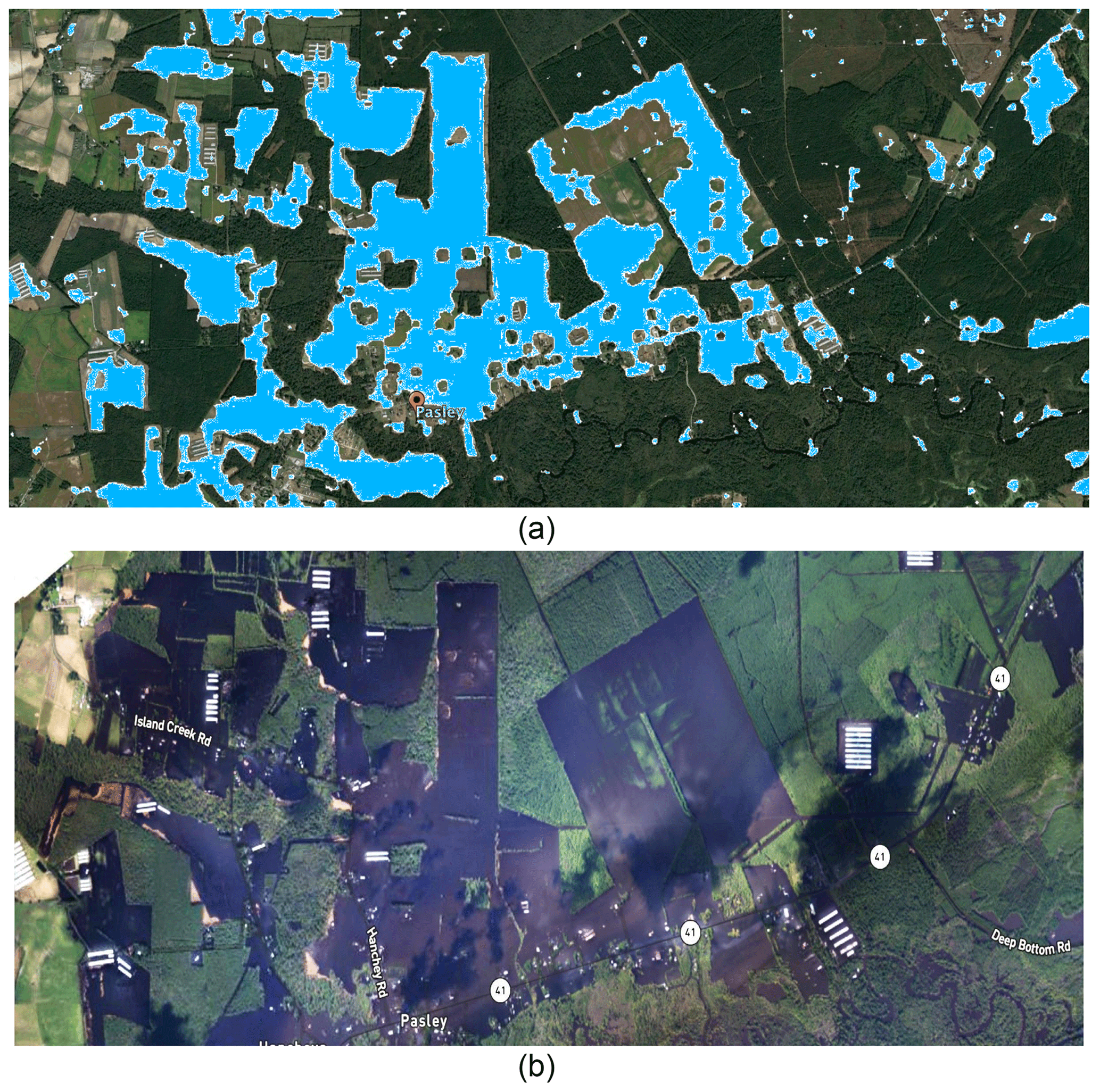
Figure 4Flooded areas detected by (a) Sentinel-1 data (light-blue-filled regions) on 19 September 2018 near Pasley, Duplin County, North Carolina (34.7854∘ N, 77.9005∘ W), and (b) photograph of the same area collected on 18 September 2018 by NOAA (https://storms.ngs.noaa.gov/storms/florence/index.html#7/35.360/-77.820, last access: October 2019). Here, dark blue regions show flooded areas.
Given these considerations, for this study we merge the FEMA and Sentinel-1 flood extent maps to generate a maximum composite flood extent map that will be used to assess the property exposure to Hurricane Florence flooding. We will refer to this dataset simply as the “maximum flood extent” in the remaining sections of the paper.
3.2 Exposure of property to Hurricane Florence flooding
Figure 5 shows the spatial distribution of the properties within our database overlaid with an image of the eye of Hurricane Florence when it made landfall. Our analysis indicates that the total area of properties affected by the maximum flood extent water was 70 964 700 m2 (e.g., physical footprint), being 17.55 % of the total area within our database. When considering only the flood extent estimated by Sentinel-1, the total area of properties affected by the flood reduces to 3.2 %, corresponding to 12 939 432 m2. In order, to quantify potential biases associated with co-registration issues or resampling procedures, we also computed the number of properties exposed to the extent of our permanent water body dataset. Our analysis shows that less than 0.2 % of properties overlapped with the permanent water bodies. Consequently, we removed these properties from our analysis.
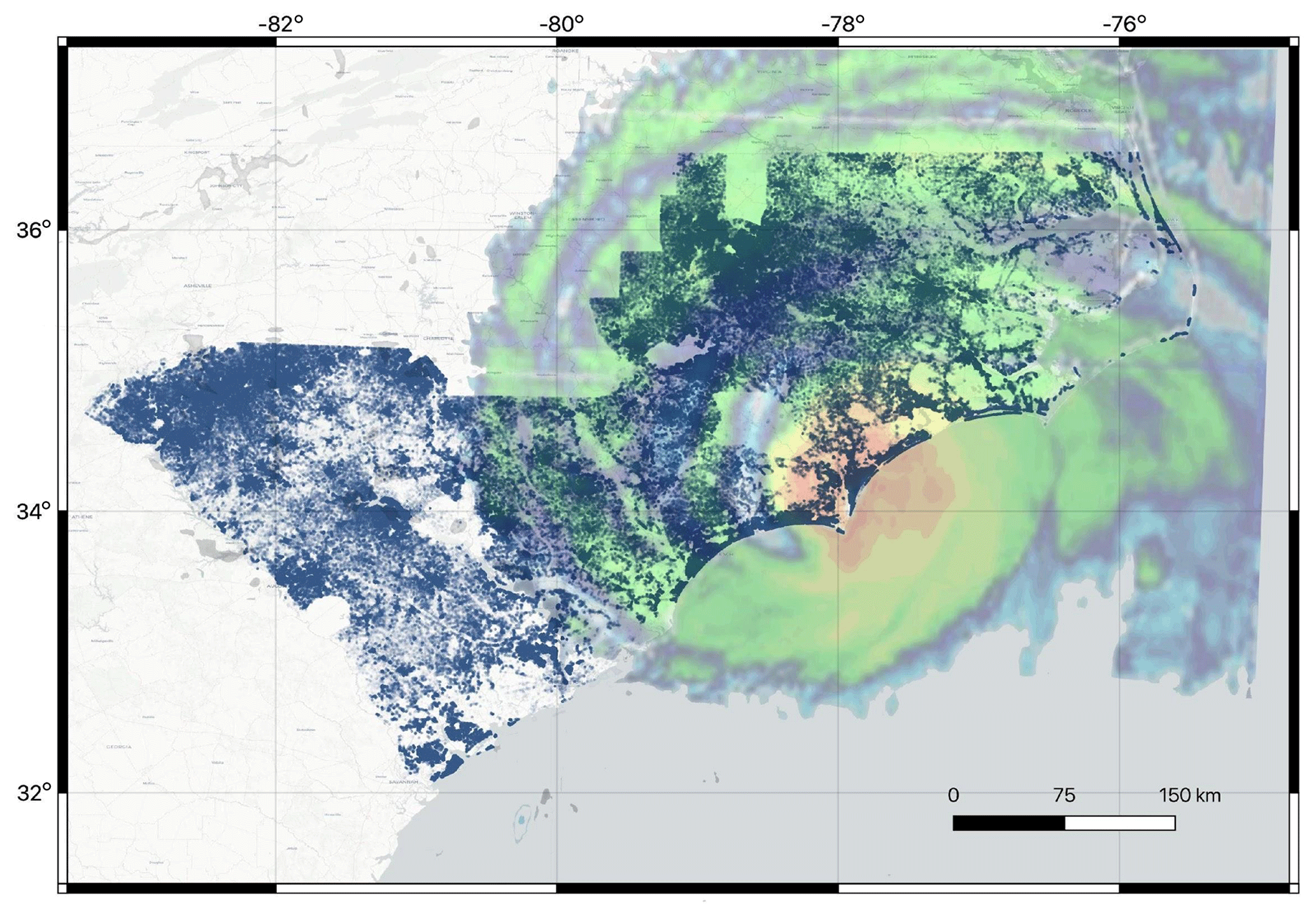
Figure 5Distribution of properties within our database used to estimate the exposed-property damage from Hurricane Florence. An image of the Hurricane Florence making landfall is also reported as a reference. ©Hurricane image courtesy: Cyclocane.
The total exposed-property value estimated using the maximum flood extent is USD 52 079 520 584 (2018 USD, corresponding to ∼9.5 % of the total property value within our database). The exposed-property value is USD 9 437 931 512 when considering only Sentinel-1 data. The exposed-property value computed over the flooded regions estimated by Sentinel-1 but not by FEMA is USD 3 278 098 601. The relatively small exposure area and property values obtained with Sentinel-1 are due to the limitations discussed above and the difficulties of SAR data to detect flooding in urban areas (e.g., Notti et al., 2018), where the basic assumption on the physical processes leading to the detection of flooded areas by Sentinel-1 is violated by the presence of dense vegetation or buildings. In this case, indeed, the radar signal will bounce on the vertical structures (e.g., buildings and trees) after being reflected by the water surface, increasing the amount of energy reaching the radar receivers rather than reducing it, as expected in the absence of vegetation or urban structures (e.g., Schumann et al., 2018; Schumann, 2018). Another reason for the underestimation of property exposure derived from Sentinel-1 data can be seen in Fig. 4. Here it is evident that Sentinel-1 detects flooding over rural and agricultural areas, where the number of properties is smaller than in highly density populated areas.
In Fig. 6 we report the distribution of the number of properties exposed to flooding as a function of the corresponding property value. A power law function (as reported in Eq. 1),
fitting the histogram is also plotted as a dashed, black line with a and n obtained from the fitting as and . The power law function selected here was chosen after testing several functions (exponential decay, logarithmic, etc.) as the one showing the highest regression coefficient (R=0.99). According to Zillow©, the median home values in North Carolina and South Carolina are, respectively, USD 184 200 (North Carolina) and USD 166 300 (South Carolina), with a median price of homes of USD 196 600 in the case of North Carolina and USD 187 800 in the case of South Carolina. We use these estimates to set to USD 200 000 as the median price within our database and evaluate the number of properties this value using Eq. (1). We find that 40 % of the properties exposed to Hurricane Florence flooding were below the threshold value. The properties valued between USD 200 000 and 500 000 account for another 25 %, whereas the properties with values between USD 500 000 and USD 1 million account for another 25 %. As a reference, the total number of properties valued below USD 200 000 represent ∼50 % of our database, those between USD 200 000 and USD 500 000 represent ∼25 %, and those between USD 500 000 and USD 1 million represent roughly 15 %.

Figure 6Distribution of the number of properties exposed to flooding as a function of property value. Dashed line represents the power law curve fitting the distribution. The parameters of the fitting power law function are reported in the top right section of the figure.
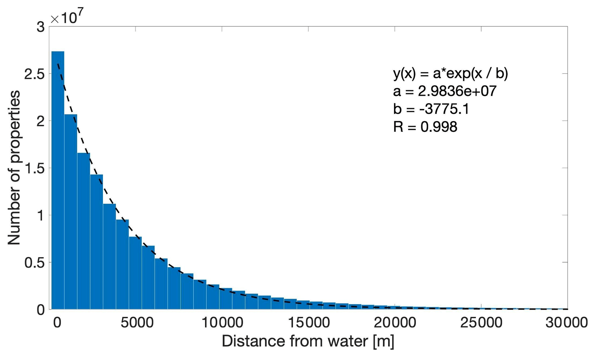
Figure 7Number of properties as a function of distance from water bodies. Dashed line represents the power law curve fitting the distribution. The parameters of the fitting power law function are also reported in the top right section of the figure.
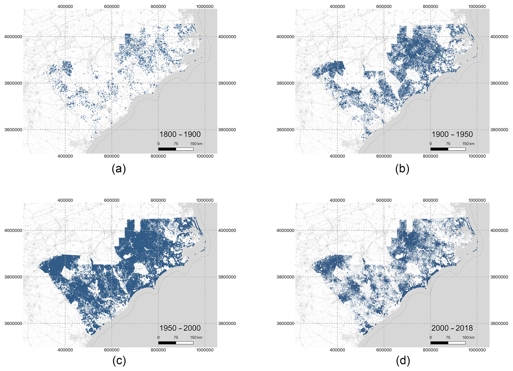
Figure 8Spatial distribution of the properties within our database that were built during the (a) 1800–1900, (b) 1900–1950, (c) 1950–2000 and (d) 2000–2018 periods.
Distance from water bodies, especially coastal and riverine bodies, is also a useful indicator of properties vulnerability and potential exposure in hurricane-prone areas. Consequently, we expanded our analysis to consider the distance of the properties that were flooded during Florence within our database from permanent water bodies (Fig. 7). Values along the x axis in the plot are obtained as the minimum distance from any of the closest element of the permanent water body mask (e.g., ocean, rivers, lakes) to each property within our database. The figure also shows the exponential decay function fitting the histogram and the corresponding fitting parameters. From this analysis, we estimate that ∼95 % of the number of properties exposed to flooding fell within 10 km from water bodies. This number increases when considering only the distance from the ocean because of the inland flooding associated with heavy precipitation. We, therefore, use the distance of 10 km as a maximum distance for studying the relationship between new properties, their distance from water bodies and the exposure to the Florence flood extent.
3.3 Impact of expansion of urban areas on property exposure
Addressing this point is crucial to account for those impacts related to urban growth and the expansion of urban areas as addressed by experts when considering the so-called expanding bull's eye effect (Ashley and Strader, 2016), in which targets of geophysical hazards, such as people and their built environments, enlarge as populations grow and spread. In this case, the bull's eye expansion does not refer to the increased storm size but rather to the area where the impact of the geophysical hazard occurs, expanding because of the urbanization process over the past decades. This concept is well synthesized in what has been named the expanding bull's eye effect (Ashley and Strader, 2016), arguing that targets – people and their built environments – of geophysical hazards enlarge as populations grow and spread. We point out that, to demonstrate their bull's eye effect, Ashley and Strader (2016) work with a semi-empirical spatio-temporal model of housing stock in tornado zones over time. A major difference between this study and that of Ashley and Strader (2016) is that in our case we have a snapshot of stock rather than a continuous record through time (i.e., annual records of all properties). This means that our dataset might be skewed toward newer properties as old buildings get replaced and that, despite the bull's eye expansion effect being evident from space, our property dataset might only capture it indirectly. With this in mind, we calculated what would have been the property area and values exposed to the Florence flood that would have occurred 10, 50 or 100 years ago by using the information contained within our database on the years when properties were built. For the purpose of this analysis, we clarify that we are assuming the same sea levels and topography of today.
Figure 8 shows the spatial distribution of the properties within our database that were built during the (a) 1800–1900, (b) 1900–1950, (c) 1950–2000 and (d) 2000–2018 periods. We considered the first period to be a 100-year one (Fig. 8a) because of the relatively small number of properties that were built then. Most of the urban growth between 1900 and 1950 (Fig. 8b) occurred inland and along the coast north of Wilmington, with a relatively small number of new properties built close to water bodies (either rivers or ocean). An explosion in new properties occurred between 1950 and 2000 (Fig. 8c), likely as a consequence of the economic stimulus following World War II. The period 2000–2018 shows a relatively smaller number of new properties with respect to the previous periods (Fig. 8d). In this regard, our analysis performed on the 10-year period of number of properties built within our database (Fig. 9) shows that before 2010 the number of houses built had been increasing exponentially (, R=0.99, with X being the year) and that the number of new properties after 2010 drastically dropped, reaching values similar to those observed before the 1950s. This might be due to the 2008 housing crisis that occurred during that period.
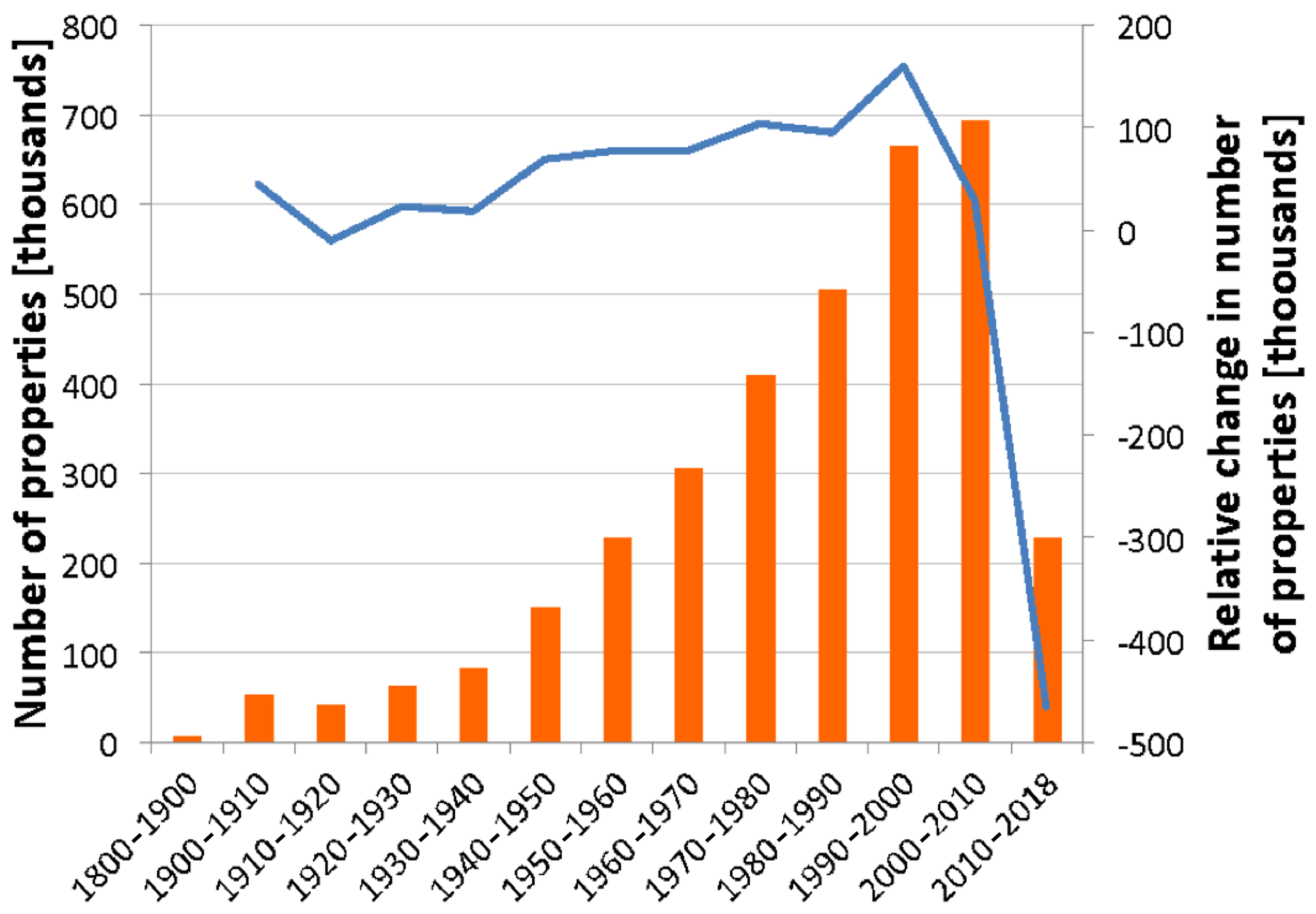
Figure 9Number of properties (in thousands) built within our data record during different decades (red bars; left axis) and relative change between two consecutive periods (blue line; right axis). Note that the number of properties built between 1800 and 1900 are aggregated as a single value because of the small number of properties built during that period.
Figure 10 shows the time series of total value of exposed property (in 2018 billion USD). The inset reports the relative change of the exposed area and value between two consecutive time steps (10 years). Consistent with the results discussed above, a relatively small increase in the exposed-property value occurs before the 1940s (from USD ∼10 billion to USD ∼12 billion). Urban expansion increases considerably after the 1940s (Fig. 8), reaching a maximum value of exposed property of USD ∼52 billion in 2018. We fitted the increase in exposed-property value after 1900 with an exponential function () and computed the coefficients providing the best fit (, b=0.167, R=0.97). The maximum relative increase is reached around the year 2000, with an increase in exposed-property value of USD ∼8 billion between two successive decades. After that, the relative change in exposed-property values decreases to those obtained in the early 1950s.
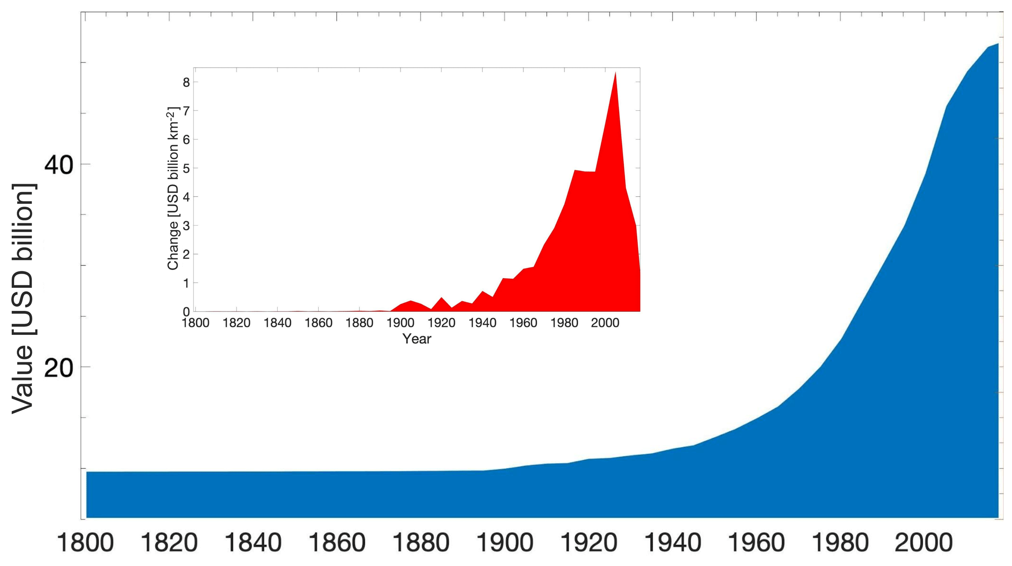
Figure 10Time series of total value of exposed buildings (in 2018 USD) to the maximum flooded extent region between 1800 and 2018. The inset shows the relative change of the exposed area and value between two consecutive time steps (10 years).
As mentioned, distance from permanent water bodies can play a critical role in terms of exposure, with flooding due to Hurricane Florence reaching properties that were up to ∼10 km from the closest water body. Therefore, we further studied how the property value evolved in terms of the distance from water bodies between 1800 and 2018. As an example, in Fig. 11 we show the distribution of properties built during different periods in proximity to Wrightsville Beach, where Hurricane Florence made landfall. The figure clearly highlights the expansion of urban areas along the coasts and water bodies, especially between 2000 and 2018. In Fig. 12 we also show the total value of exposed properties within our database as a function of distance from water bodies between 1800 and 2000 (using a 25-year time step) and for the period 2000–2018. We note that the curves referring to early decades reach a plateau within a shorter distance than those referring to later periods, with the saturation values (e.g., the value when the curve becomes flat) being of the order of 1500 m in the case of the 1975–2000 period. Differently from other periods, the one spanning between 2000 and 2018 does not show a saturation value with the distance from water bodies, with the exposed-property values continuing to increase as the distance from water increases. This is an important aspect, as it suggests that, despite the most recent decades being characterized by a relatively smaller number of new properties (Fig. 9), the potential exposure to Florence of such properties was higher because of the higher number of the exposed properties close to water bodies.
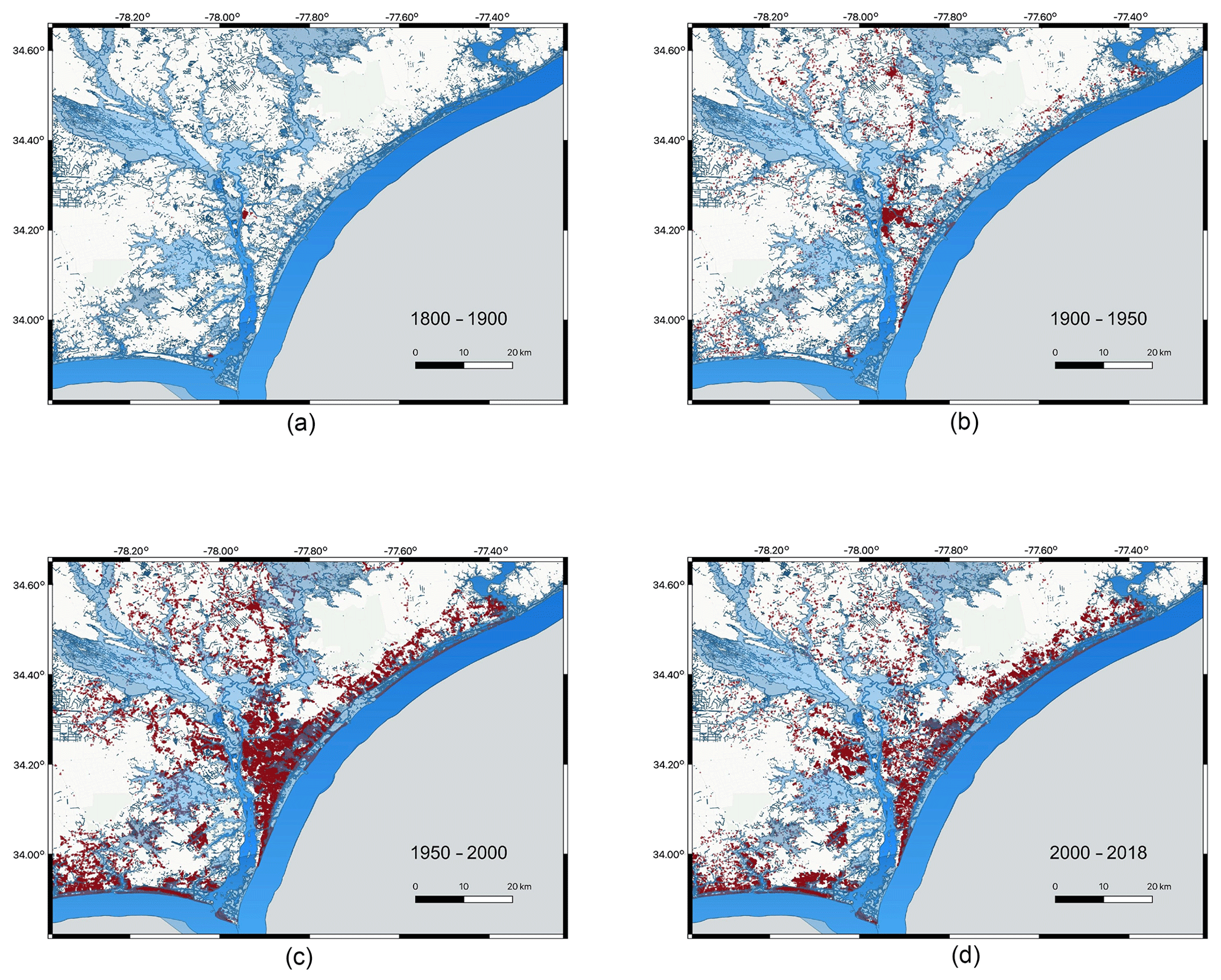
Figure 11Distribution of properties (red areas) built (a) before 1900, (b) between 1900 and 1950, (c) between 1950 and 2000, and (d) between 2000 and 2018 in proximity to Wrightsville Beach, North Carolina, where Hurricane Florence made landfall. Dark blue shows permanent water bodies, whereas light blue shows the flooded areas.
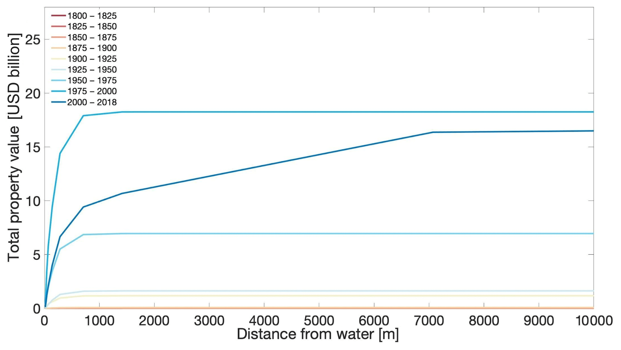
Figure 12Total value within our database of properties exposed to flooding as a function of distance from water for the different periods reported in the inset.
Increased flooding associated with sea level rise, storm surges and other extreme events has the potential to economically disrupt many areas around the world, with the most valuable real estate, densest communities and most productive economic engines situated in coastal regions. The specific goal of our study was to quantify the exposure of properties to the flooding associated with Hurricane Florence that hit the Carolinas in September 2018 and to study how the spatio-temporal evolution of new built properties along the most recent decades has impacted the property exposure. It is important to note that much of the vulnerability associated with building development in these areas should be considered independent of climate change to this point. However, moving forward, these types of storms are expected to increase in intensity and the link between climate change and potential exposure is likely to be tied more closely together. In fact, we are already seeing these trends as they relate to tidal flooding events, and one might expect that the low-probability, larger storms are likely to become more linked to our changing climate as well.
In order to properly quantify the exposure of properties to Florence flooding, we developed a maximum flood extent map from the combination of the FEMA maximum extent map (generated through the merging of high-water marks) and the flooded areas detected by means of spaceborne radar data acquired by the ESA Sentinel-1 sensors. We found that the total value of property exposed to flooding was USD ∼52 billion and that this value has increased exponentially from USD ∼10 billion (2018 USD) in the early 1900s. This is due to the increase in the number of properties that came to a halt at the beginning of the 2000s, likely as a consequence of the 2008 housing crisis, when the number of new properties built after 2010 was almost half of those built only a decade before. Despite this, the exposure to Florence flooding for those properties built after 2000 continued increasing because of the number of new properties built in proximity to permanent water bodies and coastlines.
Our work not only provide new insights for policymakers and city planners but also provides a tool to better estimate how the property market will respond to future disasters. Recent work (e.g., McAlpine and Porter, 2018; Keenan et al., 2018) has found that homes at lower elevations were being penalized on the market relative to homes at higher elevations and that houses exposed to sea level rise sell for approximately 7 % less than observably equivalent unexposed properties equidistant from the beach (Bernstein et al., 2019). For our future work, we plan to expand our analysis to other modern-day (e.g., Irma, Michael, Katrina and Sandy) and historical (e.g., Hugo in 1989) hurricanes to address similar questions to those addressed in this study. Moreover, we plan to improve the detection of maximum flood extent through the implementation of machine-learning techniques combining radar maps with tide gauge interpolated data and other ancillary information. Lastly, the combination of the knowledge on how property distribution changed over the years in conjunction with outputs of physical or probabilistic models that can separate the different contributions associated to flood due to sea level rise, storm surge and rain will allow for properly quantification of the impact of the different components of the climate–economic system on the total exposure and, eventually, damage. This will provide a crucial tool for policymakers, governments, citizens and those who are, rightly, interested in quantifying the impact of climate change on the economic and housing markets.
We used a combination of publicly available software and codes developed ad hoc for the purpose of this study. Specifically, the ESA SNAP software used to preprocess the Sentinel datasets is available at http://step.esa.int/main/download/snap-download/ (last access: 15 October 2019). We also used QGIS 3.4 to export the property data into a shapefile and to analyze the permanent water bodies and the FEMA maximum flood extent data. The software is available at https://qgis.org/en/site/forusers/download.html (last access: 15 October 2019). We developed in-house codes in MATLAB for mapping flooded areas from radar data and for performing the analysis of the exposed-property values. These are available upon request to the corresponding author at mtedesco@ldeo.columbia.edu.
Sentinel-1 data are freely available at https://earthdata.nasa.gov/about/daacs/daac-asf (last access: 15 October 2019). The dataset containing the permanent water bodies is available at https://fwsprimary.wim.usgs.gov/wetlands/apps/wetlands-mapper/ (last access: 15 October 2019). Land use land cover attributes obtained from the National Geospatial Data Asset (NGDA) Land Use Land Cover (LULC) dataset are available at (https://www.sciencebase.gov/catalog/item/581d050ce4b08da350d52363, last access: 15 October 2019). Maximum water extent by FEMA is available at https://data.femadata.com/FIMA/NHRAP/Florence/ (last access: 15 October 2019). Property value data are compiled from each individual property's county assessor in the form of the property tax assessed value and were obtained from ATTOM™ Data Solutions. Those interested in this dataset should reach out to the corresponding author (mtedesco@ldeo.columbia.edu), or data can be obtained at https://www.attomdata.com/ (last access: 15 October 2019).
The supplement related to this article is available online at: https://doi.org/10.5194/nhess-20-907-2020-supplement.
MT conceived the study and wrote the first draft of the paper. JRP and SM provided and analyzed the property data, permanent water bodies and LULC data. MT developed and implemented the code for the radar dataset. All authors contributed to the final analysis and final version of the paper.
The authors declare that they have no conflict of interest.
This article is part of the special issue “Hydroclimatic extremes and impacts at catchment to regional scales”. It is not associated with a conference.
Marco Tedesco acknowledges financial support from Columbia University through the RISE program and from the FirstStreet Foundation.
This paper was edited by Fernando Domínguez-Castro and reviewed by two anonymous referees.
Ashley, W. S. and Strader, S. M.: Recipe for disaster: How the dynamic ingredients of risk and exposure are changing the tornado disaster landscape, B. Am. Meteorol. Soc., 97, 767–786, 2016.
Bernstein, A., Gustafson, M. and Lewis, R.: Disaster on the Horizon: The Price Effect of Sea Level Rise, J. Financ. Econ., Forthcoming (as of June 2019), https://doi.org/10.2139/ssrn.3073842, 2019.
Bin, O., Crawford, T., Kruse, J., and Landry, C.: Viewscapes and Flood Hazard: Coastal Housing Market Response to Amenities and Risk, Land Econ., 84, 434–448, 2008.
Bin, O., Poulter, B., Dumas, C. F., and Whitehead, J. C.: Measuring the impact of sea level rise on coastal real estate: a hedonic property model approach, J. Reg. Sci., 51, 751–767, 2011.
Borenstein, S. and Fingerhut, H.: Most Americans see weather disasters worsening, AP-NORC Poll, 5 September 2019.
Domeneghetti, A., Schumann, G. J.-P., and Tarpanelli, A.: Preface: Remote Sensing for Flood Mapping and Monitoring of Flood Dynamics, Remote Sens., 11, 943–947, https://doi.org/10.3390/rs11080943, 2019.
FEMA: Standard Operating Procedure for Hazus Flood Level 2 Analysis, available at: https://www.fema.gov/media-library-data/1530821743439-e16c13c1f6266bbe374dc00a00ac9910/Hazus_Flood_Model_SOP_level2analysis.pdf, last access: 6 June 2019.
Fu, X., Song, J., Sun, B., and Peng, Z.: “Living on the edge”: Estimating the economic cost of sea level rise on coastal real estate in the Tampa Bay region, Florida, Ocean Coast. Manage., 133, 11–17, 2016.
Gebrehiwot, A., Hashemi-Beni, L., Thompson, G., Kordjamshidi, P., and Langan, T. E.: Deep Convolutional Neural Network for Flood Extent Mapping Using Unmanned Aerial Vehicles Data, Sensors, 19, 1486, https://doi.org/10.3390/s19071486, 2019.
Giordan, D., Notti, D., Villa, A., Zucca, F., Calò, F., Pepe, A., Dutto, F., Pari, P., Baldo, M., and Allasia, P.: Low cost, multiscale and multi-sensor application for flooded area mapping, Nat. Hazards Earth Syst. Sci., 18, 1493–1516, https://doi.org/10.5194/nhess-18-1493-2018, 2018.
Hallegatte, S., Ranger, N., Mestre, O., Dumas, P., Corfee-Morlot, J., Herweijer, C., and Wood, R. M.: Assessing climate change impacts, sea level rise and storm surge risk in port cities: a case study on Copenhagen, Climatic Change, 104, 113–137, 2011.
Huang, W., DeVries, B., Huang, C., Lang, M. W., Jones, J. W., Creed, I. F., and Carroll, M. L.: Automated Extraction of Surface Water Extent from Sentinel-1 Data, Remote Sens., 10, 797–805, https://doi.org/10.3390/rs10050797, 2018.
Huang, X., Wang, C., and Lu, J.: Understanding the spatiotemporal development of human settlement in hurricane-prone areas on the US Atlantic and Gulf coasts using nighttime remote sensing, Nat. Hazards Earth Syst. Sci., 19, 2141–2155, https://doi.org/10.5194/nhess-19-2141-2019, 2019.
Keenan, J. M., Hill, T., and Gumber, A.: Climate Gentrification: From Theory to Empiricism in Miami-Dade County, Florida, Environ. Res. Lett., 13, 054001, https://doi.org/10.1088/1748-9326/aabb32, 2018.
Kildow, J. T., Colgan, C. S., Scorse, J. D., Johnston, P., and Nichols, M.: State of the US Ocean and Coastal Economies, National Ocean Economics Program Report, 2016 Update, Middlebury Institute of International Studies at Monterey, California, 2014.
Kunthreuther, H., Wachter, S., Kousky, C. and Lacour-Little, M.: Flood Risk and the U.S. Housing Market, Working Paper, Risk Management and Decision Process Center, University of Pennsylvania, Pennsylvania, October 2018.
Manavalan, R.: SAR image analysis techniques for flood area mapping – Literature survey, Earth Sci. Inf., 10, 1–14, 2017.
McAlpine, S. A. and Porter, J. R.: Estimating the Local Impacts of Sea-Level Rise on Current Real-Estate Loses: A Housing Market Case Study in Miami-Dade, Florida, Populat. Res. Policy Rev., 36, 871–895, 2018.
Michael, J. A.: Episodic Flooding and the Cost of Sea-Level Rise, Ecol. Econ., 63, 149–159, 2007.
NOAA: National Coastal Population Report: Population Trends from 1970 to 2020, 2013.
Notti, D., Giordan, D., Caló, F., Pepe, A., Zucca, F., and Galve, J. P.: Potential and Limitations of Open Satellite Data for Flood Mapping, Remote Sens., 10, 1673, https://doi.org/10.3390/rs10111673, 2018.
Parsons, G. R. and Powell, M.: Measuring the Cost of Beach Retreat, Coast. Manage., 29, 91–103, 2001.
Roberson, M. W., Bell, A. L., Roberson, L. E., and Walker, T. A.: Geospatial analytics of Hurricane Florence flooding effects using overhead imagery, Proceedings, 10992, 1099208, https://doi.org/10.1117/12.2519242, 2019.
Schumann, G. J.-P.: Remote Sensing of Floods, Oxford Research Encyclopedia of Natural Hazard Science, UK, https://doi.org/10.1093/acrefore/9780199389407.013.265, 2018.
Schumann, G. J.-P., Neal, J. C., Mason, D. C., and Bates, P. D.: The accuracy of sequential aerial photography and SAR data for observing urban flood dynamics: A case study of the UK summer 2007 floods, Remote Sens. Environ., 115, 2536–2546, 2011.
Schumann, G. J.-P., Brakenridge, G. R., Kettner, A. J., Kashif, R., and Niebuhr, E.: Assisting Flood Disaster Response with Earth Observation Data and Products: A Critical Assessment, Remote Sens., 10, 1230, https://doi.org/10.3390/rs10081230, 2018.
Srikanto, P., Ghebreyesus, D., and Hatim, O. S.: Brief Communication: Analysis of the Fatalities and Socio-Economic Impacts Caused by Hurricane Florence, Geosciences, 9, 58–70, https://doi.org/10.3390/geosciences9020058, 2019.
Torres, R., Snoeij, P., Geudtner, D., Bibby, D., Davidson, M., Attema, E., Potin, P., Rommen, B., Floury, N., Brown, M., Navas Traver, I., Deghaye, P., Duesmann, B., Rosich, B., Miranda, N., Bruno, C., L'Abbate, M., Croci, R., Pietropaolo, A., Huchler, M., and Rostan, F.: GMES Sentinel-1 mission, Remote Sens. Environ., 120, 9–24, https://doi.org/10.1016/j.rse.2011.05.028, 2012.
UCSUSA – Union of Concerned Scientists: Underwater: Rising Seas, Chronic Floods, and the Implications for US Coastal Real Estate, available at: https://www.ucsusa.org/sites/default/files/attach/2018/06/underwater-analysis-full-report.pdf, last access: 19 June 2019.